Model-Based Predictive Rotor Field-Oriented Angle Compensation for Induction Machine Drives

Abstract

In this paper, a model-based predictive rotor field-oriented angle compensation approach is proposed for induction machine drives. Indirect rotor field-oriented control is widely used in induction machine drives for its simple implementation and low cost. However, the accuracy of the rotor field-oriented angle is affected by variable parameters such as the rotor resistance and inductance. An inaccurate rotor field-oriented angle leads to a degradation of the torque and dynamic performance, especially in the high-speed flux-weakening region. Therefore, the d-axis and q-axis currents in the rotation reference frame are predicted based on the model and compared with the feedback current to correct the rotor field-oriented angle. To improve the stability and robustness, the proposed predictive algorithm is based on the storage current, voltage, and velocity data. The algorithm can be easily realized in real-time. Finally, the simulated and experimental results verify the algorithm’s effectiveness on a 7.5 kW induction machine setup.

1. Introduction

Indirect rotor field-oriented control (IRFOC) is widely used in induction machine drives because of its high performance in the base speed and field-weakening region. The control scheme of IRFOC is shown in Figure 1. Currently, the flux level and torque control in IRFOC are the research highlights in the field-weakening region [1,2,3,4,5,6]. The solutions are based on the accuracy of the rotor field-oriented angle. However, the rotor field-oriented method based on the integration of the rotor angular velocity and rotor slip angular velocity in IRFOC is affected by variations in parameters such as the rotor resistance. The rotor resistance varies with temperature and can be more than twice that of the normal resistance at 25 °C. The well-known solution to rotor field-oriented inaccuracy is parameter identification [5,6,7,8,9,10] and observers [11,12,13,14,15]. In [5,6], a magnetizing curve of induction in the field-weakening region and saturated region is proposed. Off-line parameter identification methods are proposed in [7,8]. A simple calculation based on the specification of an induction machine is introduced in [9]. These methods are useful and easy to apply in industry. Online parameter identification schemes are proposed in [10,11]. Solutions to address the parameter sensitivity problem in speed sensorless control of induction machines have been proposed, such as a sliding mode observer [12,13,14,15], a low-pass filter [16], square-wave voltage injection [17], and model reference adaptive control [18]. These algorithms require considerable computational resources and mainly aim to reduce the risk of instability phenomena. However, in the IRFOC of induction machines, the inaccurate field orientation caused by variable parameters is due to not only the instability but also the load capacity and dynamic performance.

Model-based predictive control (MPC) for machine drives and power electronics is an alternative control strategy that has gained attention in recent years. This approach can be used to address multivariable system constraints and nonlinearities in a very intuitive way [19]. Therefore, MPC has been successfully used for different applications, such as power converters connected to resistor–inductor (RL) loads [20], power electronics fault tolerance [21,22,23], energy management of electric vehicles [24,25], autonomous vehicle control [26,27], and high-performance drives for AC machines [28,29,30,31,32]. In [28], an MPC-based vector control method named GTV-MPTC for induction machines is proposed to cause the instantaneous torque to reach its reference value at the end of the next control period. The weighting factors in MPC are eliminated by investigating the relationship between the torque and stator flux to avoid tedious tuning work in [29]. However, the impact of variable parameters such as stator and rotor resistors is not given. In [30,31,32], MPC is used to improve the dynamic performance and reduce torque ripples in permanent-magnet synchronous motors (PMSM) drives. Compared to the vector control of induction machines, the control of PMSMs does not require a calculation of the slip velocity. Therefore, the rotor flux orientation for PMSMs is easy and accurate using a speed sensor.

In this paper, a compensation approach based on a model predictive algorithm of the rotor field-oriented angle error is proposed for IRFOC of induction machines. The d-axis and q-axis currents in the rotation reference frame are predicted and compared with the currents by current sensors to correct the rotor flux oriented angle. To improve the stability and robustness, the proposed predictive algorithm is based on the current, voltage, and velocity data stored in the memory. The algorithm can be realized easily in real-time. After compensation of the rotor field-oriented angle error, the output torque and current control performance can be improved. In Section 2, the mathematical model of IRFOC is introduced. Section 3 demonstrates the proposed model-based predictive algorithm and its implementation based on the stored data. The simulated results are shown in Section 4. Finally, the experimental results are presented to verify the proposed method in Section 5.

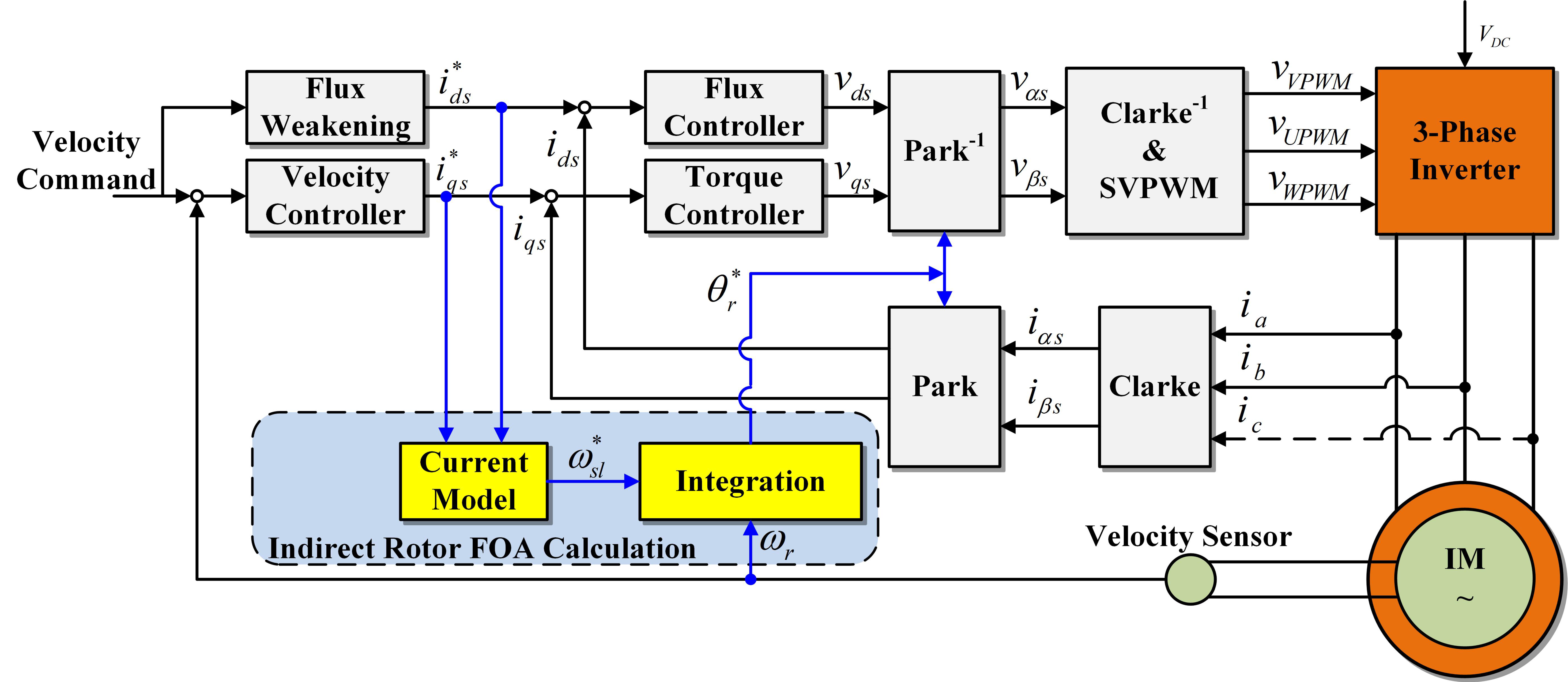
2. Induction Machine Control Model

2.1. Induction Machine Model

The dynamic model of the induction machine is important for the study of transient analysis on computers. If the currents in the rotating reference frame are selected as the main variables, then the state space stator voltage equations in the rotating reference frame can be obtained as

$$\left[\begin{array}{l}{v}_{qs}\\ v_{ds}\end{array}\right]=\left[\begin{array}{cccc}\begin{array}{c}{R}_s+L_{s}p\\ -{\omega }_e{L}_s\end{array}& \begin{array}{c}{\omega }_e{L}_s\\ R_s+L_{s}p\end{array}& \begin{array}{l}{L}_{m}p\\ {\omega }_e{L}_m\end{array}& \begin{array}{l}{\omega }_e{L}_m\\ L_{m}p\end{array}\end{array}\right]\left[\begin{array}{c}{i}_{qs}\\ i_{ds}\\ i_{qr}\\ i_{dr}\end{array}\right]$$

(1)

where $v_{qs}$, $v_{ds}$, $i_{qs}$, and $i_{ds}$ are the stator q-axis and d-axis voltages and currents, respectively; $i_{qr}$ and $i_{dr}$ are the rotor q-axis and d-axis currents, respectively; $R_s$ and $L_s$ the stator resistance and inductance, respectively; $L_m$ is the magnetizing inductance; ${\omega }_e$ is the synchronous rotating angular velocity; and $p$ is the differential factor.

The rotor flux linkage expressions in terms of the currents can be written as

$$\left[\begin{array}{l}{\psi }_{qr}\\ {\psi }_{dr}\end{array}\right]=\left[\begin{array}{cccc}\begin{array}{l}{L}_m\\ 0\end{array}& \begin{array}{l}0\\ L_m\end{array}& \begin{array}{c}{L}_r+L_m\\ 0\end{array}& \begin{array}{c}0\\ L_r+L_m\end{array}\end{array}\right]\left[\begin{array}{c}{i}_{qs}\\ i_{ds}\\ i_{qr}\\ i_{dr}\end{array}\right],$$

(2)

where ${\psi }_{qr}$ and ${\psi }_{dr}$ are the rotor q-axis and d-axis flux linkages, respectively. $L_r$ is the inductance of the rotor.

The d-axis is located on the rotor flux linkage in the IRFOC. Therefore, ${\psi }_{qr}=0$ and ${\psi }_r={\psi }_{dr}$. By Equation (2), the rotor current in Equation (1) can be substituted as

$$v_{qs}=R_s{i}_{qs}+\delta L_s\frac{d{i}_{qs}}{dt}+{\omega }_e{L}_s{i}_{ds}+\frac{{\omega }_e{L}_m}{L_r}({\psi }_r-L_m{i}_{ds}),$$

(3)

$$v_{ds}=R_s{i}_{ds}+L_s\frac{d{i}_{ds}}{dt}-{\omega }_e\delta L_s{i}_{qs}+\frac{L_m}{L_r}\frac{d({\psi }_r-L_m{i}_{ds})}{dt},$$

(4)

where $\delta =1-\frac{L_m^2}{L_s{L}_r}$.

The rotor flux in the IRFOC can be expressed as

$$\frac{L_r}{R_r}\frac{d{\psi }_r}{dt}+{\psi }_r=L_m{i}_{ds},$$

(5)

Then, Equation (5) is substituted into Equation (3) to obtain

$$v_{qs}=R_s{i}_{qs}+\delta L_s\frac{d{i}_{qs}}{dt}+{\omega }_e{L}_s{i}_{ds}-\frac{{\omega }_e{L}_m}{R_r}\frac{d{\psi }_r}{dt}$$

(6)

And Equation (4) can be given as

$$v_{ds}=R_s{i}_{ds}+\delta L_s\frac{d{i}_{ds}}{dt}-{\omega }_e\delta L_s{i}_{qs}+\frac{L_m}{L_r}\frac{d{\psi }_r}{dt}$$

(7)

2.2. Discrete-Time Model

The first-order approximation, as shown in Equation (8), is usually used to transfer the continuous-time model to the discrete-time model.

$$\frac{dx}{dt}=\frac{x(k)-x(k-1)}{T_s}$$

(8)

where $T_s$ is the sample period. By substituting Equation (8) into Equations (6) and (7), the discrete-time model of the induction machine control system can be obtained as

$$\begin{array}{l}{v}_{qs}(k)=(R_s+\frac{\delta L_s}{T_s})i_{qs}(k)+{\omega }_e{L}_s{i}_{ds}(k)-\\ \frac{\delta L_s}{T_s}{i}_{qs}(k-1)+\frac{{\omega }_e{L}_m}{R_r{T}_s}({\psi }_r(k)-{\psi }_r(k-1))\end{array}$$

(9)

$$\begin{array}{l}{v}_{ds}(k)=(R_s+\frac{\delta L_s}{T_s})i_{ds}(k)-\frac{\delta L_s}{T_s}{i}_{ds}(k-1)-\\ {\omega }_e\delta L_s{i}_{qs}(k)+\frac{L_m}{L_r{T}_s}({\psi }_r(k)-{\psi }_r(k-1))\end{array}$$

(10)

The rotor flux varies slowly compared to the variation in the current and voltage. Therefore, Equations (9) and (10) can be simplified as

$$v_{qs}(k)=(R_s+\frac{\delta L_s}{T_s})i_{qs}(k)-\frac{\delta L_s}{T_s}{i}_{qs}(k-1)+{\omega }_e{L}_s{i}_{ds}(k)$$

(11)

$$v_{ds}(k)=(R_s+\frac{\delta L_s}{T_s})i_{ds}(k)-\frac{\delta L_s}{T_s}{i}_{ds}(k-1)-{\omega }_e\delta L_s{i}_{qs}(k)$$

(12)

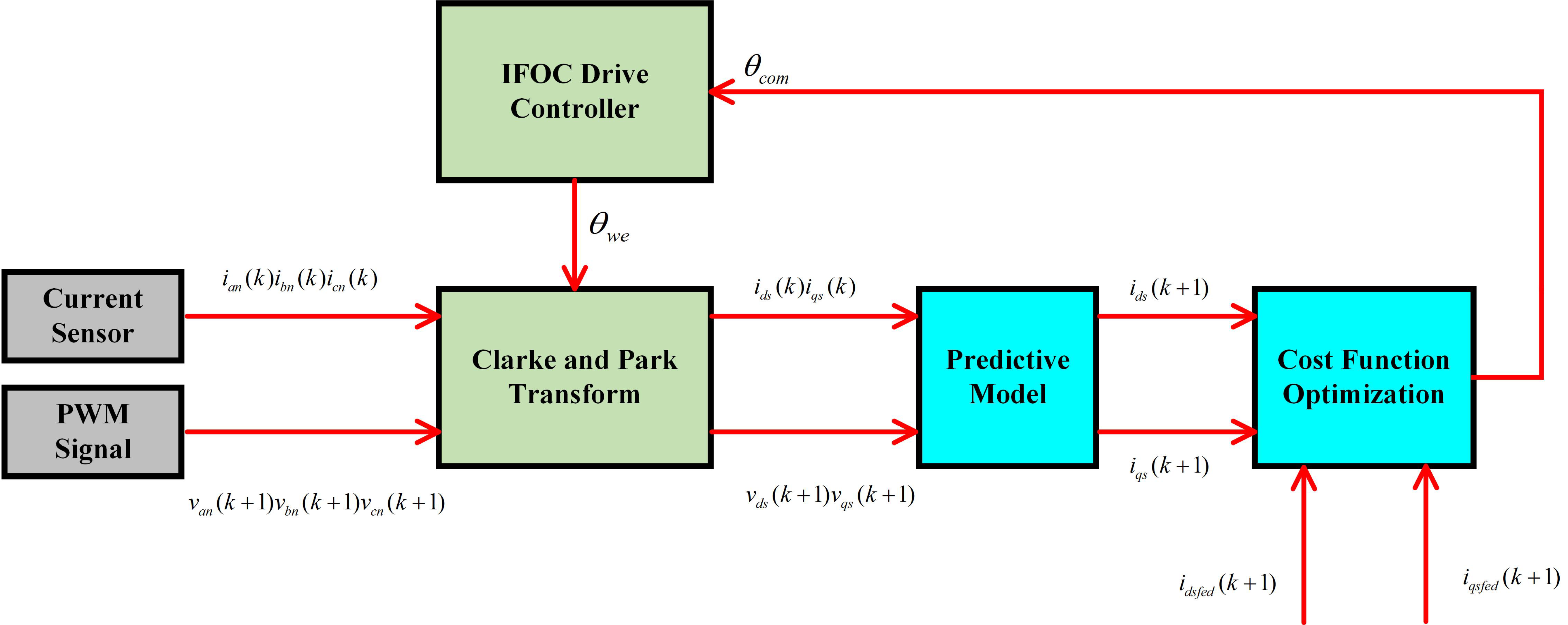
3. Model-Based Predictive Algorithm and Implementation

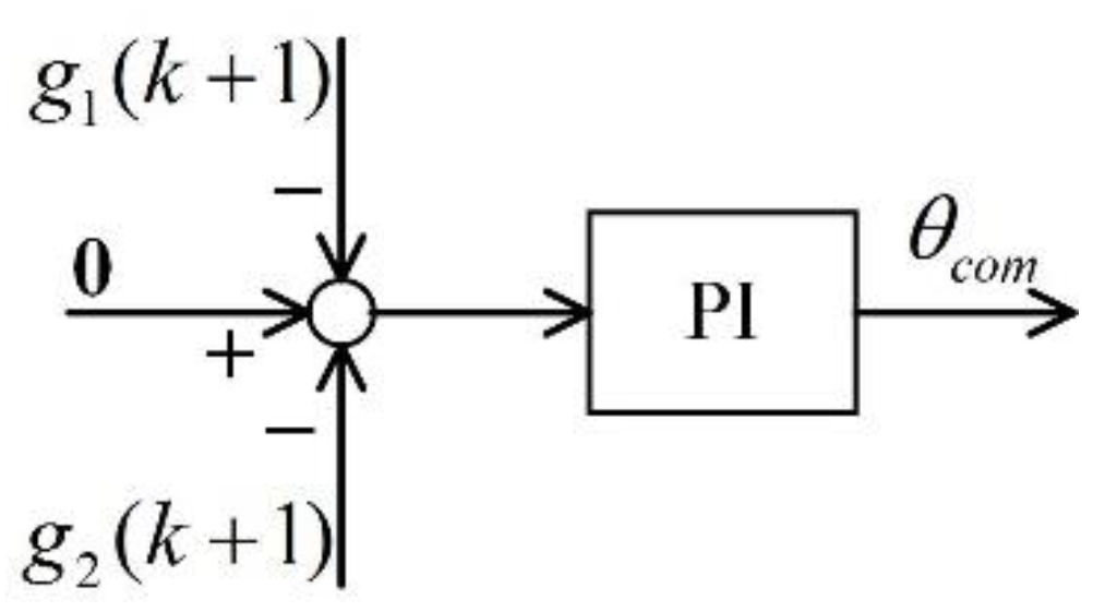
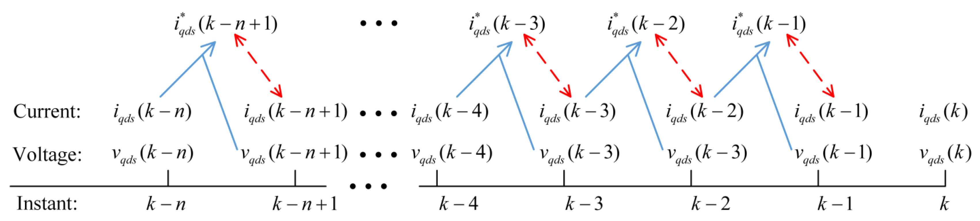
3.1. Model-Based Predictive Algorithm

In the discrete model, based on Equations (11) and (12), the d-axis and q-axis currents at the k + 1 instant are predicted by

$$\left\{\begin{array}{c}(R_s+\frac{\delta L_s}{T_s})i_{qs}(k+1)+{\omega }_e{L}_s{i}_{ds}(k+1)=\frac{\delta L_s}{T_s}{i}_{qs}(k)+v_{qs}(k+1)\\ -{\omega }_e\delta L_s{i}_{qs}(k+1)+(R_s+\frac{\delta L_s}{T_s})i_{ds}(k+1)=\frac{\delta L_s}{T_s}{i}_{ds}(k)+v_{ds}(k+1)\end{array}\right.$$

(13)

Then,

$$\left\{\begin{array}{c}{i}_{qs}(k+1)=\frac{C\times A-D\times E}{A^2+F\times E}\\ i_{ds}(k+1)=\frac{C\times F+D\times A}{A^2+F\times E}\end{array}\right.$$

(14)

where $A=R_s+\frac{\delta L_s}{T_s}$, $C=\frac{\delta L_s}{T_s}{i}_{qs}(k)+v_{qs}(k+1)$, $D=\frac{\delta L_s}{T_s}{i}_{ds}(k)+v_{ds}(k+1)$, $E={\omega }_e(k)L_s$, and $F={\omega }_e(k)\delta L_s$. The voltages $v_{ds}(k+1)$ and $v_{qs}(k+1)$ are the d-axis and q-axis voltages at k + 1 instant, respectively. When the IRFOC is realized in a digital signal processor (DSP) or microcontroller unit (MCU), $v_{ds}(k+1)$ and $v_{qs}(k+1)$ can be obtained by the pulse width modulation (PWM) duty cycle at the k instant because the PWM duty cycle calculated at the k instant will be active at the k + 1 instant. Therefore, $v_{ds}(k+1)$ and $v_{qs}(k+1)$ do not need to be predicted.

Based on (14), the predicted currents, $i_{qs}(k+1)$ and $i_{ds}(k+1)$, at the k + 1 instant can be obtained without the rotor field-oriented angle. According to Equations (13) and (14), the stator resistance $R_s$ is needed and varies with temperature. However, the variation in the stator resistance can be neglected because it is very small compared with the other parts of Equation (14). Therefore, the stator resistance on the motor plate can be used. The predictive model control diagram is shown in Figure 2. ${\theta }_{com}$ in Figure 2 is the compensated angle of the rotor field-oriented error; ${\theta }_{we}$ is the rotor field-oriented angle with compensation; $i_{an}(k)$, $i_{bn}(k)$, and $i_{cn}(k)$ are the three-phase currents at the k instant; $v_{an}(k+1)$, $v_{bn}(k+1)$, and $v_{cn}(k+1)$ are the phase voltages at the k + 1 instant; $i_{dsfed}(k+1)$ and $i_{qsfed}(k+1)$ are the d-axis and q-axis currents based on the feedback current at the k + 1 instant.

The cost function is $g(k+1)$.

$$g(k+1)=p_1{g}_1(k+1)+p_2{g}_2(k+1)+\dots +p_n{g}_n(k+1)$$

(15)

where $p_1$, $p_2$ … $p_n$ are the weighting coefficients and $p_1+p_2+\dots +p_n=1$. The functions $g_1(k+1)$, $g_2(k+1)$ … $g_n(k+1)$ are the different optimization objective cost functions. Here,

$$g_1(k+1)=i_{ds}^{*}(k+1)-i_{ds}(k+1)$$

(16)

$$g_2(k+1)=i_{qs}^{*}(k+1)-i_{qs}(k+1)$$

(17)

If the rotor field-oriented angle is accurate, then $g_1(k+1)=0$ and $g_2(k+1)=0$. Therefore, $g(k+1)=0$. If the $g(k+1)\ne 0$, then the angle ${\theta }_{we}$ will be compensated by ${\theta }_{com}$. The proportional integral (PI) regulator shown in Figure 3 is used to linearly tune the ${\theta }_{com}$. Zero is used as the input of the PI regulator. It means that the rotor field-oriented angle error is none.

3.2. Implemented Algorithm

The currents in the IRFOC are always in a dynamic state. The current at the k + 1 instant cannot be sensed at present. Therefore, an approach algorithm that takes advantage of the historic current and voltage is proposed.

The historic data of the current, voltage, and field-oriented angle, e.g., $i(k-n)$, $i(k-n+1)$…$i(k-1)$, $i(k)$, as shown in Figure 4, can be recorded in the random-access memory (RAM) of the DSP or MCU. According to (14), the current at the instant $k-n+1$ can be predicted with the current $i(k-n)$ and $v(k-n+1)$. That is

$$\left\{\begin{array}{c}{i}_{qs}^{*}(k-n+1)=\frac{C{}^{\prime }\times A-D{}^{\prime }\times E{}^{\prime }}{A^2+F{}^{\prime }\times E{}^{\prime }}\\ i_{ds}^{*}(k-n+1)=\frac{C{}^{\prime }\times F{}^{\prime }+D{}^{\prime }\times A}{A^2+F{}^{\prime }\times E{}^{\prime }}\end{array}\right.$$

(18)

where $C{}^{\prime }=\frac{\delta L_s}{T_s}{i}_{qs}(k-n)+v_{qs}(k-n+1)$, $D{}^{\prime }=\frac{L_s}{T_s}{i}_{ds}(k-n)+v_{ds}(k-n+1)$, $E{}^{\prime }={\omega }_e(k-n)L_s$, $F{}^{\prime }={\omega }_e(k-n)\delta L_s$, $i_{qs}^{*}(k-n+1)$ and $i_{ds}^{*}(k-n+1)$ are the predicted currents at the instant k − n.

The accuracy of the predicted current at the next instant can be improved with the data at the previous instants. The current and voltage are always in a dynamic state because the period of the current and voltage sample is very short and the closed-loop control period is usually the same as the sample period. Therefore, the predicted current is not stable enough to tune ${\theta }_{com}$. By using the saved data, a filter for the predicted current can be used to improve the stability of the predicted and feedback current as

$$i_{qds}^{*}=\frac{i_{qds}^{*}(k-4)+i_{qds}^{*}(k-3)+i_{qds}^{*}(k-2)+i_{qds}^{*}(k-1)}{4}$$

(19)

$$i_{qds}=\frac{i_{qds}(k-4)+i_{qds}(k-3)+i_{qds}(k-2)+i_{qds}(k-1)}{4}$$

(20)

where $i_{qds}^{*}=i_{qs}^{*}-j{i}_{ds}^{*}$ and $i_{qds}^{}=i_{qs}^{}-j{i}_{ds}^{}$ are the predicted current and the actual feedback current, respectively. Then, according to Equations (16) and (17), the cost function can be calculated. Finally, ${\theta }_{com}$ can be tuned using the PI regulator in Figure 3.

4. Simulation Results

4.1. System Description

Simulations were performed in the below-based speed region and the field-weakening region based on the IRFOC with a speed sensor. The rotor field angle is usually calculated by (21) and (22) in IRFOC.

$${\theta }_r={\displaystyle \int {\omega }_{r}dt}+{\displaystyle \int {\omega }_{sl}dt}$$

(21)

$${\omega }_{sl}=\frac{1}{t_r}\times \frac{i_{qs}^{*}}{i_{ds}^{*}}$$

(22)

where ${\theta }_r$ is the rotor field angle, ${\omega }_r$ is the actual electric angular velocity of the rotor, which can usually be obtained with a photoelectric encoder or rotating transformer, ${\omega }_{sl}$ is the slip angular velocity, $t_r$ is the rotor time constant and $t_r=L_r/R_r$. $R_r$ is the resistance of the rotor, $i_{qs}^{*}$ is the torque current command, and $i_{ds}^{*}$ is the magnetic current command. To reflect the inaccuracy of the rotor field orientation, the slip angular velocity is calculated with different rotor resistances, namely,$0.5R_r$, $0.8R_r$, and $1.5R_r$. The specifications of the simulated and experimental induction machines are shown in

Table 1. Specification of the simulated and experimental induction machines.

Machine Type	3 ph IM	Stator leakage inductance	3.3 mH
Rated power	7.5 kW	Rotor leakage inductance	5.6 mH
Rated speed	1450 rpm	Magnetizing inductance	56.4 mH
Maximum speed	12,000 rpm	Inertia	0.029 kgm2
Rated frequency	50 Hz	Number of pole pairs	2
Rated torque at rated speed	48.8 Nm	Rated DC-line voltage	540 V
Stator resistance	0.374Ω	Rated rotor flux level	0.73 Wb
Rotor resistance	0.267Ω	Rated current	18.8 A

.

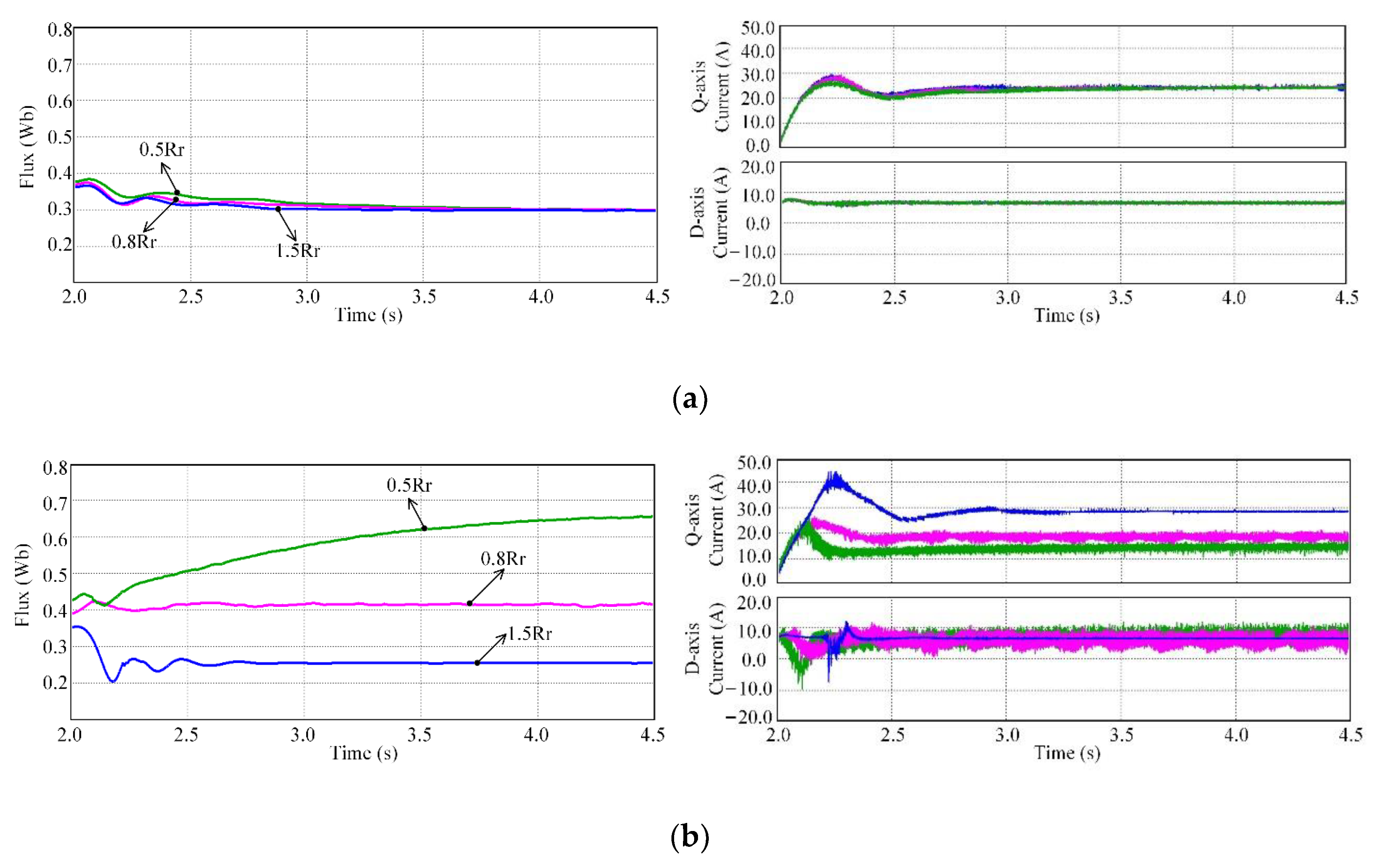
4.2. Simulated Results

Simulations were performed with the Saber simulator. Figure 5 shows the simulated results at 1200 rpm. In the IRFOC, the d-axis current, referred to as the magnetic current, is kept constant in the below-based speed region. According to Equation (5), the rotor flux should be kept constant. A step load is set at 2.0 s with 30 Nm and at 4.0 s with 60 Nm. Figure 5a–c depicts the simulated results when the rotor resistance $R_r^{*}$ is used in the slip angular velocity calculation is set as $0.5R_r$, $0.8R_r$ and $1.5R_r$, respectively. The rotor field-oriented angle is compensated from 1.0 s. The rated flux level is set to 0.73 Wb based on the motor parameters. The flux level varies because of the inaccurate rotor field-oriented angle without compensation. This effect can lead to the degradation of dynamic and stable performance. After compensation, we observe that the flux intensity under the three simulation conditions could reach 0.73 Wb at 2.0 s. The flux level could be kept almost constant during the load step.

According to Equation (18), the predictive model needs stator resistance and inductance. Inductance is almost constant. The variation in the stator resistance is neglected in the proposed algorithm. To verify that the neglect is accepted, a simulation was performed. In the simulation, the stator resistance was changed from 0.374 Ω to 0.748 Ω linearly, and the rotor resistance was set to $0.5R_r$. A step load is also set at 2.0 s with 30 Nm and at 4.0 s with 60 Nm. Compared with the simulated results in Figure 5a, the rotor flux and compensated angle indicate little difference, as shown in Figure 6. The flux level with angle error compensation, regardless of whether the stator resistance is changed, is much better than that without compensation. Although the maximum deviation of the compensated angle is almost 2.5 rad when the stator resistance changed to twice the nominal resistance, the deviation of the rotor flux level is only 0.03 Wb. In the application, this small difference of the rotor flux level could be neglected, and the algorithm proposed here is almost not affected by the variation in the stator resistance.

In the IRFOC, the q-axis current reflects the developed torque when the motor runs at a constant speed. Therefore, the q-axis current should be proportional to the torque. That is, the q-axis current with a 60 Nm load should be twice the value with a 30 Nm load at 1200 rpm. The q-axis current with different loads is presented in Figure 7. After compensation, the q-axis current is changed from approximately 15 A to 30 A when the load rises from 30 Nm to 60 Nm regardless of the $R_r^{*}$ set. However, with no compensation, the q-axis current is different from the same load and is not proportional to the torque. The simulated current is compared in

Table 2. Q-axis current comparison.

	Without Compensation			With Compensation
	${\mathit{R}}_{\mathit{r}}^{*}=0.5{\mathit{R}}_{\mathit{r}}$	${\mathit{R}}_{\mathit{r}}^{*}=0.8{\mathit{R}}_{\mathit{r}}$	${\mathit{R}}_{\mathit{r}}^{*}=1.5{\mathit{R}}_{\mathit{r}}$	${\mathit{R}}_{\mathit{r}}^{*}=0.5{\mathit{R}}_{\mathit{r}}$	${\mathit{R}}_{\mathit{r}}^{*}=0.8{\mathit{R}}_{\mathit{r}}$	${\mathit{R}}_{\mathit{r}}^{*}=1.5{\mathit{R}}_{\mathit{r}}$
$i_{qs1}$(A)	17.1	15.01	17.9	14.9	14.92	14.95
$i_{qs2}\left(\mathrm{A}\right)$	26.1	26.5	42.2	30.1	30	30.15
$\mathrm{ratio}(i_{qs2}/i_{qs1})$	1.52	1.77	2.35	2.02	2.01	2.02

.

In Table 2, $R_r^{*}$ is the rotor resistance, which is used to calculate the slip angular velocity in the program; $R_r$ is the actual resistance of the induction machine; $i_{qs1}$ and $i_{qs2}$ are the values of the q-axis current when the loads are 30 Nm and 60 Nm, respectively. If the rotor field orientation is accurate, then the ratio of $i_{qs2}$ and $i_{qs1}$ should be 2. It can be seen that the q-axis current is not proportional to the load when the rotor resistance is not the actual value. After compensation, the q-axis current is almost proportional to the load.

Figure 8 shows the simulation results at 3000 rpm. A step load at 20 Nm was set at 2.0 s. When $R_r^{*}=0.5R_r$, the speed could no longer be kept at 3000 rpm without compensation. This is different from the simulation result at 1200 rpm shown in Figure 7 because the voltage is limited to the supply torque current in the field-weakening region if the rotor flux level is not sufficiently reduced, as shown in Figure 8b. The actual flux without compensation when $R_r^{*}=0.5R_r$ was much higher than the normal level. Therefore, the voltage could not supply enough q-axis current when the speed was 3000 rpm, and then the speed was decreased. This finding means that an inaccurate field-oriented angle can affect the maximum output torque of induction machines. This results of q-axis current can also be seen in the following experimental results at 1200 rpm. Although the flux levels with compensation are not constant, the variable in Figure 8a is much smaller than that without compensation, as shown in Figure 8b.

Figure 9 compares the waveform with and without the proposed compensation. In the simulation, the rotor resistance began to change from 0.268 Ω to 0.536 Ω linearly at the instant of 2.0 s during the following 2 s interval. Then, the rotor resistance was changed back to 0.268 Ω linearly at the instant of 4.0 s during the next 2 s interval. After compensation, the torque, rotor flux, and q-axis current are almost the same. There are some fluctuations in the flux, especially when the resistance was changed instantly. This change is mainly because the compensation of the proposed algorithm requires some time to realize. In practice, the rotor resistance cannot be changed so fast. The proposed algorithm has enough time to regulate the slip coefficient. The simulation at 3000 rpm yielded similar results, as shown in Figure 10.

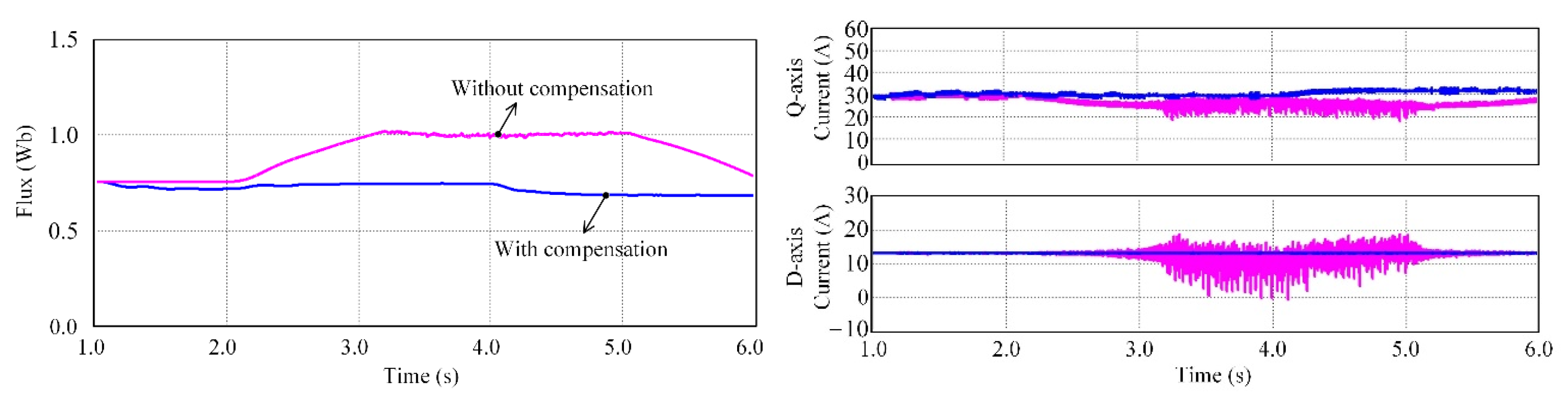
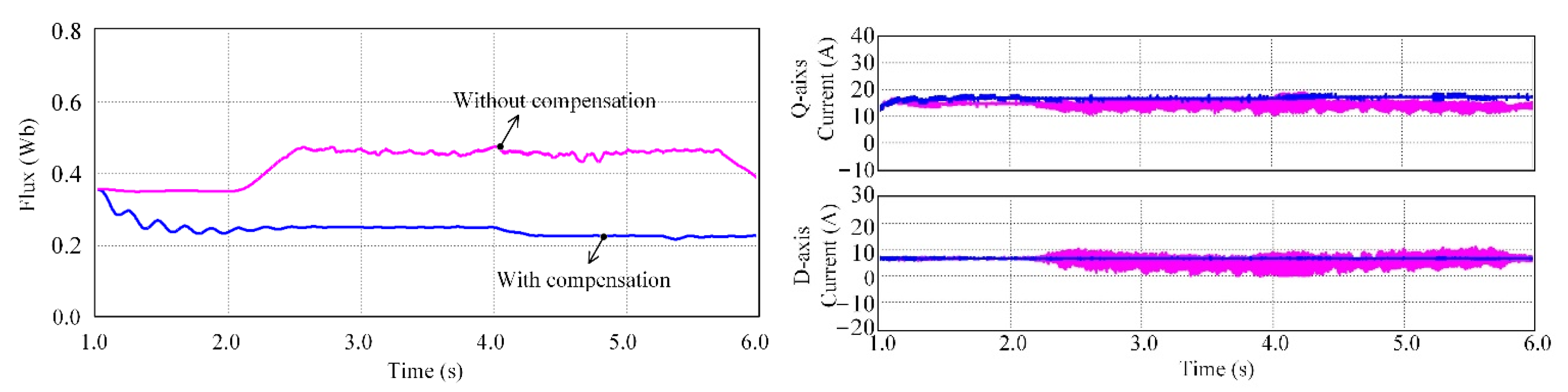
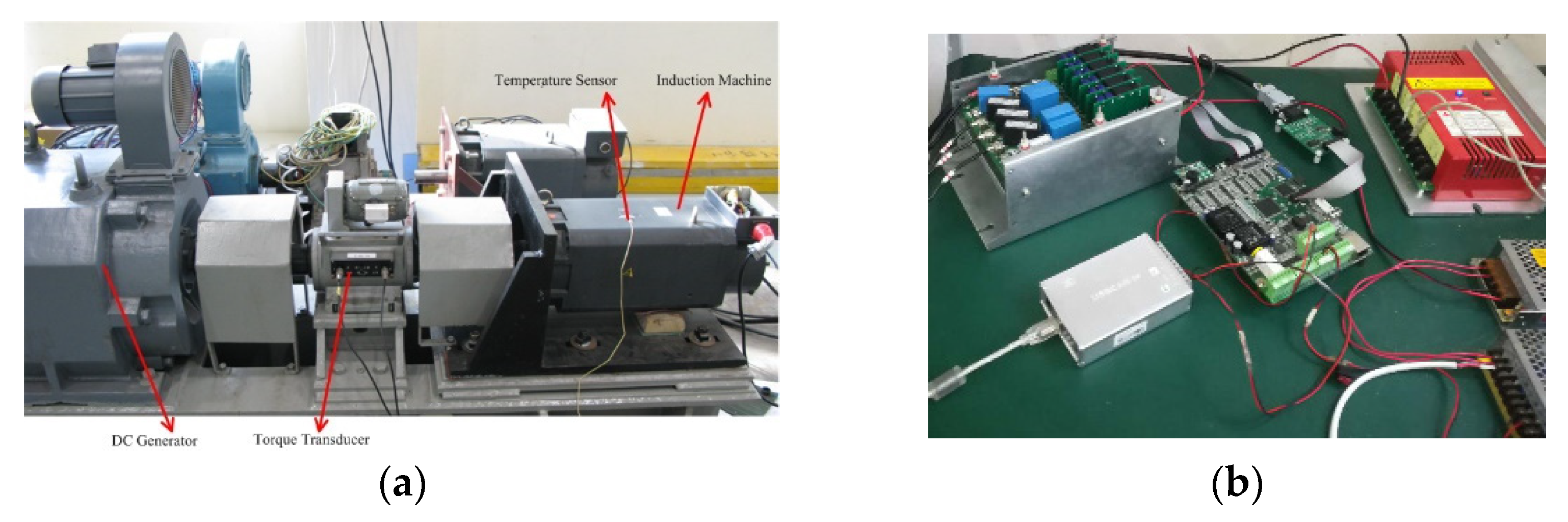
5. Experimental Results

Experiments were performed on the setup, as shown in Figure 11. A 7.5 kW spindle motor was used, and its parameters are shown in Table 1. The DC generator was used as a load in the high-speed region. The output torque can be obtained by the torque transducer, which was equipped between the spindle motor and the DC generator. A DSP TMS320F28377D (Texas Instruments, Texas, USA), which is a two core MCU was used to realize the proposed algorithm and IRFOC algorithm. A CPLD EPM240T100C5N (Altera, California, USA) was used to realize PWM. In the experiment, the PWM frequency was 10 kHz. The current sample and control frequency was 20 kHz. The phase currents were obtained by the two current sensors on the power converter board.

In the experiment, the maximum q-axis current was set to $3\sqrt{2}{i}_{rated}$. As the simulation shows, the q-axis current was not proportional to the load at the same flux level when the field-oriented angle is inaccurate. The q-axis current comparative experiment results are given in Figure 12 at 1200 rpm with different loads. The torque was applied by a DC generator. The q-axis current was calculated by the DSP and stored in RAM. Therefore, the q-axis current of the experiment was read by the DSP and transferred to a computer. The experimental results are similar to the simulated results shown in Table 2. After compensating for the rotor flux oriented angle error, the q-axis current is proportional to the load torque and is almost the same regardless of which rotor resistance was used to calculate the slip angular velocity.

If the field-oriented angle is not accurate, the maximum torque will decrease, especially in the flux weakening region. The maximum output torque at different speeds was recorded, as shown in Figure 13. The maximum torque decreased with increasing speed when the rotor resistance used in the slip angular velocity calculation was not accurate. After compensation, the output torque was increased.

6. Conclusions

This paper focuses on the correction of the field-oriented inaccuracy by a model predictive method in induction machine drives, including the base speed region and field-weakening region. The inaccuracy of the field-oriented control will lead to the actual flux variation, which could be larger or smaller than the reference value. Furthermore, the flux level variation will decrease the output torque and degrade the dynamic performance and current control regulator, especially in the field-weakening region. Therefore, a q-axis and d-axis current predictive method-based correction method for the field-oriented angle is proposed in this paper. To easily realize the proposed method in real-time, the data, such as the current, voltage and velocity used in MPC, are stored in the RAM of the DSP. The effectiveness of this approach is verified by simulations and experiments on a 7.5 kW induction machine setup.

References

1. Lin, F.J.; Liao, Y.H.; Lin, J.R.; Lin, W.T. Interior Permanent Magnet Synchronous Motor Drive System with Machine Learning-Based Maximum Torque per Ampere and Flux-Weakening Control. Energies 2021, 14, 346. [Google Scholar] [CrossRef]
2. Wu, C.; Yang, J.; Li, Q. GPIO-Based Nonlinear Predictive Control for Flux-Weakening Current Control of the IPMSM Servo System. Energies 2020, 13, 1716. [Google Scholar] [CrossRef] [Green Version]
3. Zhou, K.; Ai, M.; Sun, D.; Jin, N.; Wu, X. Field Weakening Operation Control Strategies of PMSM Based on Feedback Linearization. Energies 2019, 12, 4526. [Google Scholar] [CrossRef] [Green Version]
4. Marques, G.D.; Iacchetti, M.F. Field-Weakening Control for Efficiency Optimization in a DFIG Connected to a DC-Link. IEEE Trans. Ind. Electron. 2016, 63, 3409–3419. [Google Scholar] [CrossRef]
5. Wang, K.; Yao, W.; Chen, B.; Shen, G.; Lee, K.; Lu, Z. Magnetizing Curve Identification for Induction Motors at Standstill Without Assumption of Analytical Curve Functions. IEEE Trans. Ind. Electron. 2014, 62, 2144–2155. [Google Scholar] [CrossRef]
6. Ruan, J.Y.; Wang, S.M. Magnetizing Curve Estimation of Induction Motors in Single-phaseMagnetization Mode Considering Differential Inductance Effect. IEEE Trans. Power Electron. 2015, 31, 497–506. [Google Scholar] [CrossRef]
7. Al-Jufout, S.A.; Al-Rousan, W.H.; Wang, C. Optimization of Induction Motor Equivalent Circuit Parameter Estimation Based on Manufacturer’s Data. Energies 2018, 11, 1792. [Google Scholar] [CrossRef] [Green Version]
8. Alonge, F.; Cirrincione, M.; D’Ippolito, F.; Pucci, M.; Sferlazza, A. Parameter Identification of Linear Induction Motor Model in Extended Range of Operation by Means of Input-Output Data. IEEE Trans. Ind. Appl. 2013, 50, 959–972. [Google Scholar] [CrossRef]
9. Guimaraes, J.; Bernardes, J.; Hermeto, A.; Bortoni, E. Parameter determination of asynchronous machines from manufacturer data sheet. IEEE Trans. Energy Convers. 2014, 29, 689–697. [Google Scholar] [CrossRef]
10. Liu, Y.; Fang, J.; Tan, K.; Huang, B.; He, W. Sliding Mode Observer with Adaptive Parameter Estimation for Sensorless Control of IPMSM. Energies 2020, 13, 5991. [Google Scholar] [CrossRef]
11. Wang, K.; Chen, B.; Shen, G.; Yao, W.; Lee, K.; Lu, Z. Online Updating of Rotor Time Constant Based on Combined Voltage and Current Mode Flux Observer for Speed-Sensorless AC Drives. IEEE Trans. Ind. Electron. 2013, 61, 4583–4593. [Google Scholar] [CrossRef]
12. Bao, D.; Wu, H.; Wang, R.; Zhao, F.; Pan, X. Full-Order Sliding Mode Observer Based on Synchronous Frequency Tracking Filter for High-Speed Interior PMSM Sensorless Drives. Energies 2020, 13, 6511. [Google Scholar] [CrossRef]
13. Wang, C.; Cao, D. New Sensorless Speed Control of a Hybrid Stepper Motor Based on Fuzzy Sliding Mode Observer. Energies 2020, 13, 4939. [Google Scholar] [CrossRef]
14. Comanescu, M. Design and Implementation of a Highly Robust Sensorless Sliding Mode Observer for the Flux Magnitude of the Induction Motor. IEEE Trans. Energy Convers. 2016, 31, 649–657. [Google Scholar] [CrossRef]
15. Dominguez, J.R. Discrete-Time Modeling and Control of Induction Motors by Means of Variational Integrators and Sliding Modes—Part II: Control Design. IEEE Trans. Ind. Electron. 2015, 62, 6183–6193. [Google Scholar] [CrossRef]
16. Stojic, D.; Milinkovic, M.; Veinovic, S.; Klasnic, I. Improved Stator Flux Estimator for Speed Sensorless Induction Motor Drives. IEEE Trans. Power Electron. 2015, 30, 2363–2371. [Google Scholar] [CrossRef]
17. Yoon, Y.D.; Sul, S.K. Sensorless Control for Induction Machines Based on Square-Wave Voltage Injection. IEEE Trans. Power Electron. 2014, 29, 3637–3645. [Google Scholar] [CrossRef]
18. Smith, A.N.; Gadoue, S.M.; Finch, J.W. Improved Rotor Flux Estimation at Low Speeds for Torque MRAS-Based Sensorless Induction Motor Drives. IEEE Trans. Energy Convers. 2015, 31, 270–282. [Google Scholar] [CrossRef] [Green Version]
19. Vazquez, S.; Leon, J.I.; Franquelo, L.G.; Rodriguez, J.; Young, H.; Marquez, A.; Zanchetta, P. Model Predictive Control: A Review of Its Applications in Power Electronics. IEEE Ind. Electron. Mag. 2014, 8, 16–31. [Google Scholar] [CrossRef]
20. Yaramasu, V.; Rivera, M.; Wu, B.; Rodriguez, J. Model Predictive Current Control of Two-Level Four-Leg Inverters—Part I: Concept, Algorithm, and Simulation Analysis. IEEE Trans. Power Electron. 2012, 28, 3459–3468. [Google Scholar] [CrossRef]
21. Barrero, F.; Bermudez, M.; Duran, M.J.; Salas, P.; Gonzalez-Prieto, I. Assessment of a Universal Reconfiguration-less Control Approach in Open-Phase Fault Operation for Multiphase Drives. Energies 2019, 12, 4698. [Google Scholar] [CrossRef] [Green Version]
22. Guzman, H.; Duran, M.J.; Barrero, F.; Zarri, L.; Bogado, B.; Prieto, I.G.; Arahal, M.R. Comparative Study of Predictive and Resonant Controllers in Fault-Tolerant Five-Phase Induction Motor Drives. IEEE Trans. Ind. Electron. 2016, 63, 606–617. [Google Scholar] [CrossRef]
23. Druant, J.; Vyncke, T.; Melkebeek, J.A. Adding inverter fault detection to model-based predictive control for flying-capacitor inverters. IEEE Trans. Ind. Electric. 2015, 62, 2054–2063. [Google Scholar] [CrossRef]
24. Uebel, S.; Murgovski, N.; Baker, B.; Sjoberg, J. A Two-Level MPC for Energy Management Including Velocity Control of Hybrid Electric Vehicles. IEEE Trans. Veh. Technol. 2019, 68, 5494–5505. [Google Scholar] [CrossRef]
25. Buerger, J.; East, S.; Cannon, M. Fast Dual-Loop Nonlinear Receding Horizon Control for Energy Management in Hybrid Electric Vehicles. IEEE Trans. Control. Syst. Technol. 2018, 27, 1060–1070. [Google Scholar] [CrossRef]
26. Alcala, E.; Puig, V.; Quevedo, J.; Cayuela, V.P.; Casin, J.Q. TS-MPC for Autonomous Vehicles Including a TS-MHE-UIO Estimator. IEEE Trans. Veh. Technol. 2019, 68, 6403–6413. [Google Scholar] [CrossRef]
27. Liniger, A.; Lygeros, J. Real-Time Control for Autonomous Racing Based on Viability Theory. IEEE Trans. Control. Syst. Technol. 2019, 27, 464–478. [Google Scholar] [CrossRef] [Green Version]
28. Zhang, Y.; Yang, H. Generalized Two-Vector-Based Model-Predictive Torque Control of Induction Motor Drives. IEEE Trans. Power Electron. 2015, 30, 3818–3829. [Google Scholar] [CrossRef]
29. Zhang, Y.; Yang, H. Two-Vector-Based Model Predictive Torque Control Without Weighting Factors for Induction Motor Drives. IEEE Trans. Power Electron. 2016, 31, 1381–1390. [Google Scholar] [CrossRef]
30. Akpunar, A.; Iplikci, S. Runge-Kutta Model Predictive Speed Control for Permanent Magnet Synchronous Motors. Energies 2020, 13, 1216. [Google Scholar] [CrossRef] [Green Version]
31. Bao, G.; Qi, W.; He, T. Direct Torque Control of PMSM with Modified Finite Set Model Predictive Control. Energies 2020, 13, 234. [Google Scholar] [CrossRef] [Green Version]
32. Richter, J.; Doppelbauer, M. Predictive Trajectory Control of Permanent-Magnet Synchronous Machines With Nonlinear Magnetics. IEEE Trans. Ind. Electron. 2016, 63, 3915–3924. [Google Scholar] [CrossRef]
Figure 1. Control diagram of induction machine IRFOC.
Energies 14 02049 g001
Figure 2. Control diagram of model-based predictive rotor field-oriented angle compensation.
Energies 14 02049 g002
Figure 3. PI regulator used to tune the θ c o m .
Energies 14 02049 g003
Figure 4. Proposed implemented algorithm diagram.
Energies 14 02049 g004
Figure 5. Flux and compensated angle at 1200 rpm with 30 Nm and 60 Nm step loads at 2.0 s and 4.0 s, respectively. (a) R r * = 0.5 R r ; (b) R r * = 0.8 R r ; (c) R r * = 1.5 R r .
Energies 14 02049 g005aEnergies 14 02049 g005b
Figure 6. Rotor flux and compensated angle at 1200 rpm with the variable stator resistance.
Energies 14 02049 g006
Figure 7. The q-axis current comparative waveforms at 1200 rpm with a 30 Nm load at 2.0 s and 60 Nm load at 4.0 s. (a) Current with compensation; (b) Current without compensation.
Energies 14 02049 g007
Figure 8. Rotor flux, q-axis current, and d-axis current comparative waveforms at 3000 rpm with a 20 Nm load at 2.0 s. (a) Rotor flux and d/q current with compensation; (b) Rotor flux and d/q current without compensation.
Energies 14 02049 g008
Figure 9. Rotor flux, d-axis, and q-axis current comparative waveforms at 1200 rpm with a 60 Nm load.
Energies 14 02049 g009
Figure 10. Rotor flux, d-axis, and q-axis current comparative waveforms at 3000 rpm with a 15 Nm load.
Energies 14 02049 g010
Figure 11. Experiment setup. (a) is the induction machine and load. and (b) is the control and power board.
Energies 14 02049 g011
Figure 12. Q-axis current at 1200 rpm with 30 Nm, and 60 Nm loads. (a) R r * = 0.5 R r ; (b) R r * = 0.8 R r ; (c) R r * = 1.5 R r .
Energies 14 02049 g012
Figure 13. Maximum output torque from 1000 rpm to 6000 rpm.
Energies 14 02049 g013