Article

Study of the Thermal Conductivity of Soft Magnetic Materials in Electric Traction Machines

Institute of Electrical Machines (IEM), RWTH Aachen University, Schinkelstraße 4, 52062 Aachen, Germany
*
Author to whom correspondence should be addressed.
Energies 2021, 14(17), 5310; https://doi.org/10.3390/en14175310
Submission received: 30 July 2021 / Revised: 18 August 2021 / Accepted: 20 August 2021 / Published: 26 August 2021
(This article belongs to the Special Issue Performance of Induction Machines)

Abstract

:
The power density of traction drives can be increased with advanced cooling systems or reduced losses. In induction machines with housing and shaft cooling, the produced heat in the stator and rotor winding system needs to be extracted over the rotor and stator lamination. The influence of soft magnetic material parameters, such as texture, thickness or alloy components on the magnetization and loss behavior, are well studied. Studies about influencing factors on the thermal conductivity are hard to find. Within this study, eight different soft magnetic materials are analyzed. An analytical approach is introduced to calculate the thermal conductivity. Temperature-dependent measurements of the electric resistivity are performed to obtain sufficient data for the analytical approach. An experimental approach is performed. The thermal diffusivity, density, and specific heat capacity are determined. An accuracy study of all measurements is performed. The analytical and the experimental approach show good agreement for all materials, except very thin specimens. The estimated measurement error of those specimens has high values. The simplified case study illustrates the significant influence of the different soft magnetic materials on the capability to extract the heat in the given application.

1. Introduction

Increasing the power density of highly utilized traction drives is a frequently discussed research topic. The reduction of losses or the improvement of the heat dissipation capabilities are both potential measures to address this target. A significant influencing factor on the overall efficiency of a traction drive is the selection of the soft magnetic material. The influence of structural material parameters on the efficiency of the electric drive is well studied [1,2]. Eddy losses play a significant role in traction applications, due to their high frequency dependency. In order to reduce this loss share, silicon (Si) and aluminum (Al) can be added as alloy components to the iron matrix. The specific electric resistance ρ el is increased, leading to a reduced loss contribution of the eddy losses [1,2]. A direct dependency between the electron contribution of the thermal conductivity k e and the specific electric resistance ρ el can be found in the Wiedemann–Franz law:
k e = L 0 ϑ ρ el ,
with the Lorenz number L 0 and the temperature ϑ . As shown within this study, the rule is not fully applicable for alloys, but already indicates a negative impact of increased Si and Al alloy components on the thermal conductivity k. Several influencing thermal parameters, such as the heat transition in the air gap, the interfaces between lamination and housing, the impregnation goodness or the end winding correlation are well studied within the literature [3,4]. A fundamental understanding of the influencing factors of structural soft magnetic parameters on the thermal behavior of electric machines is rare to find. Correlations or validated data for the thermal conductivity of soft magnetic material are not frequently studied. Exact knowledge about the thermal conductivity of soft magnetic materials is crucial for its selection. The selection is especially challenging in the case that the soft magnetic material is placed within the main heat dissipating path. A well suited example for such an application is an Induction Motor (IM) with housing and direct shaft cooling, such as that introduced in [5].
Within this study, an analytical as well as an experimental approach is introduced to obtain data for the thermal conductivity of soft magnetic materials. Eight different soft magnetic materials with different Al and Si content are selected, according to Table 1. The name of the material, an Acronym (Acr.) with the material number from one to eight, the silicon weight content, the aluminum weight content and the nominal thickness are added to the overview. Measurements of the electric resistivity ρ el in dependency of the temperature ϑ are performed to have sufficient data input for the analytical approach. For the experimental approach, the thermal conductivity k m is determined using an indirect measurement technique.
k m ( ϑ ) = a ( ϑ ) · ρ ( ϑ ) · c p ( ϑ )
The thermal diffusivity a ( ϑ ) is measured using a Laser Flash Analysis (LFA). The density of the material ρ is measured at room temperature, using the Archimedes principle. A simple model is used to adapt the gained data in dependency of the temperature. A modified model of the Kopp–Neumann law is utilized to determine the specific thermal heat capacity c p ( ϑ ) of the materials. All measurements and models are developed for a temperature range between room temperature and 225   C . The results of the thermal conductivity in dependency of the temperature k ( ϑ ) are compared between the indirect measurement and the analytical approach. The results are used to investigate the influence of the material choice on the thermal heat dissipating capabilities of a traction drive. An IM with direct shaft cooling and housing cooling, as introduced in [5], is selected as a reference for this simplified case study.
A study is performed to evaluate the accuracy of the measurement according to [6]. The accuracy is defined as the closeness of agreement between a measured quantity value and a true quantity value of the measurand. The accuracy is not a quantity and cannot be given as a numerical quantity value according to [6]. In order to analyze the accuracy, an estimation of a possible measurement error is performed. This error estimation is aimed to represent the worst possible measurement error. It includes systematic and random measurement errors. The absolute value of the estimated error of a variable x is labeled with Δ x . The estimated relative measurement error δ x can be expressed with the following:
δ x = Δ x x .
Please note the difference between accuracy and precision. Precision is the closeness of agreement between indications or measured quantity values obtained by replicate measurements on the same or similar objects under specified conditions [6]. In order to gain good measurement results, both precise and accurate measurement results are necessary. The precision throughout the study shows very good values. The coefficient of variation c v is used for investigating the measurement precision. The c v is calculated by a division of the standard deviation of a measurement sequence and the gained average value.

2. Analytical Formula for the Thermal Conductivity

The two main mechanisms of heat transfer in metallic alloys, such as soft magnetic material, are the phonon k p and the electron thermal conductivity k e . The total value for the analytical approach k calc can be calculated as follows:
k calc ( ϑ ) = k p ( ϑ ) + k e ( ϑ )
The mechanism can be subdivided into different scatter processes between phonons, electrons and imperfections. A good overview of the resulting interactions is given in [7,8]. This study mainly uses the correlations as introduced in [8]. The most important assumptions and derivations of the correlations are discussed in the following.

2.1. Phonon Thermal Conductivity

An important quantity for the description of phonon scatter processes is the material-dependent Debye temperature θ D . Several publications address the identification of this variable. Different values are identified in dependency of the used methodology as discussed in [9]. The average value of θ D = 418   K has developed as the state of the art [8,10,11] and is used in this study. The thermal resistance of the phonon-phonon scatter W p p is defined by the following:
W p p ( ϑ ) = A · ϑ θ D .
The constant A is calculated by Julian’s modification of the Liebfried–Schlömann equation [8,10,12]. The authors in [10] conclude that the alloy components have a minor influence on the thermal resistance of the phonon–phonon scatter. The values of A = 0.412   m K / W and θ D = 418   K for pure α -iron can be used for the calculation. The authors in [11] suggest a correction term for ϑ > θ D to consider the thermal expansion. The temperature range in this study is limited to values of 498 K . The correction term is neglected because the maximum influence is 0.2 % in the considered temperature range. The phonon–phonon scatter W p p can be simplified using the introduced simplifications as follows:
W p p ( ϑ ) = 9.86 × 10 5 m / W · ϑ
The formulation of the thermal resistance of the phonon–electron scatter W p e shows a temperature dependency. A formulation of W p e at a temperature that is equal to the Debye temperature θ D is given with the following:
W p e = 2.69 × 10 2 m K / W
Additional therms need to be considered for temperatures below the Debye temperature θ D [10,11]. In this study, only small differences from the Debye temperature are considered, and the additional therms are neglected. A similar simplification is used in [8] for alloys. The thermal resistance of the phonon–impurity scatter W p i describes the interaction between impurities such as the alloys and the Fe-lattice. The process can be modeled as follows [8]:
W p i = B · i c a , i · Γ i ,
with an experimental constant B, the impurity parameter Γ i and the atomic content c a , i of each alloy i. The value of B is given in [8] with B = 1.36 × 10 2   m K / W . The impurity factor Γ can be calculated based on weighted ratios of the molar masses and the molar volumes between the alloy contents i and the Fe-lattice. The values for nine different alloys are given in [8]. The value for silicon, aluminum, and manganese is equal to 0.59 , 0.05 , and zero, respectively. This means that the influence of aluminum is almost negligible, and the influence of manganese is not present. The phonon thermal conductivity k p can be calculated as the inverse of a sum of the three influences W p p ( ϑ ) , W p e , and W p i :
k p ( ϑ ) = 9.86 × 10 5 / K · ϑ + 2.69 × 10 2 + 1.36 × 10 6 · i c a , i · Γ i 1 W / ( m   K ) .

2.2. Electron Thermal Conductivity

The first process that influences the electron thermal conductivity is the electron-phonon scatter. The process is described by the thermal resistance W e p [10]:
W e p ( ϑ ) = ρ el Fe ( ϑ ) L ( ϑ ) · ϑ .
The ideal electric resistivity is the electric resistivity of pure iron ρ el Fe ( ϑ ) in this application. The value can be calculated utilizing the following [8,13]:
ρ el Fe ( ϑ ) = 2.4 + 3.65 × 10 2 / K · ϑ + 64 × 10 9 / K 3 · ϑ 3   μ Ω   c m .
Please note that there seems to be a typo in the original source in [13] because the values do not match the measurement data presented in the publication. This typo is corrected in [8]. The values of [8] are used in this study and presented in Equation (11). The Lorenz number L 0 = 2.443 × 10 8 W   Ω / K 2 is modified by a temperature-dependent therm [10] in Equation (10):
L ( ϑ ) = L 0 · 1 e ϑ / 159.3   K .
The second considered electron scattering process is the electron–impurity scatter that is represented by W e i :
W e i ( ϑ ) = ρ el 0 ( ϑ ) L 0 · ϑ ,
with the residual electrical resistivity ρ el 0 ( ϑ ) = ρ el ( ϑ ) ρ el Fe ( ϑ ) as a difference between the electric resistivity of the alloy ρ el ( ϑ ) and the electric resistivity of pure iron ρ el Fe ( ϑ ) . The electric resistivity of an alloy can be calculated utilizing Matthiessen’s rule as follows:
ρ el ( ϑ ) = ρ el Fe ( ϑ ) + i ρ el i c a , i ,
The calculated values utilizing this formula deviate from measurement results as discussed in [10], due to the independency of the electric resistivity ρ el i from the temperature. The authors [10] propose an improved formulation:
ρ el ( ϑ ) = ρ el Fe ( ϑ ) + i ρ el i ( ϑ ) c a , i ,
The estimation of the necessity of utilizing the improved equation in comparison to the Matthiessen’s rule is not possible for this application. The error estimation in [10] is based on values of the electric resistivity of the alloy at 4   K and based on Cr and Ni alloys. While Equation (14) is preferred, due to the simple availability of the electric resistivity of the alloy components ρ el i , Equation (15) seems to give more accurate results. Within this study, the electric resistivity of the alloys is measured over the temperature range and compared to the simplified equation. The final value of the electron thermal conductivity k e ( ϑ ) can be calculated with:
k e ( ϑ ) = ρ el Fe ( ϑ ) L ( ϑ ) · ϑ + ρ el 0 ( ϑ ) L 0 · ϑ 1 .

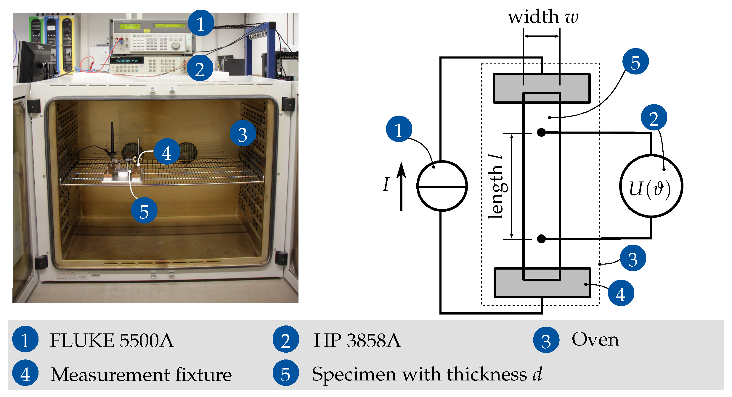
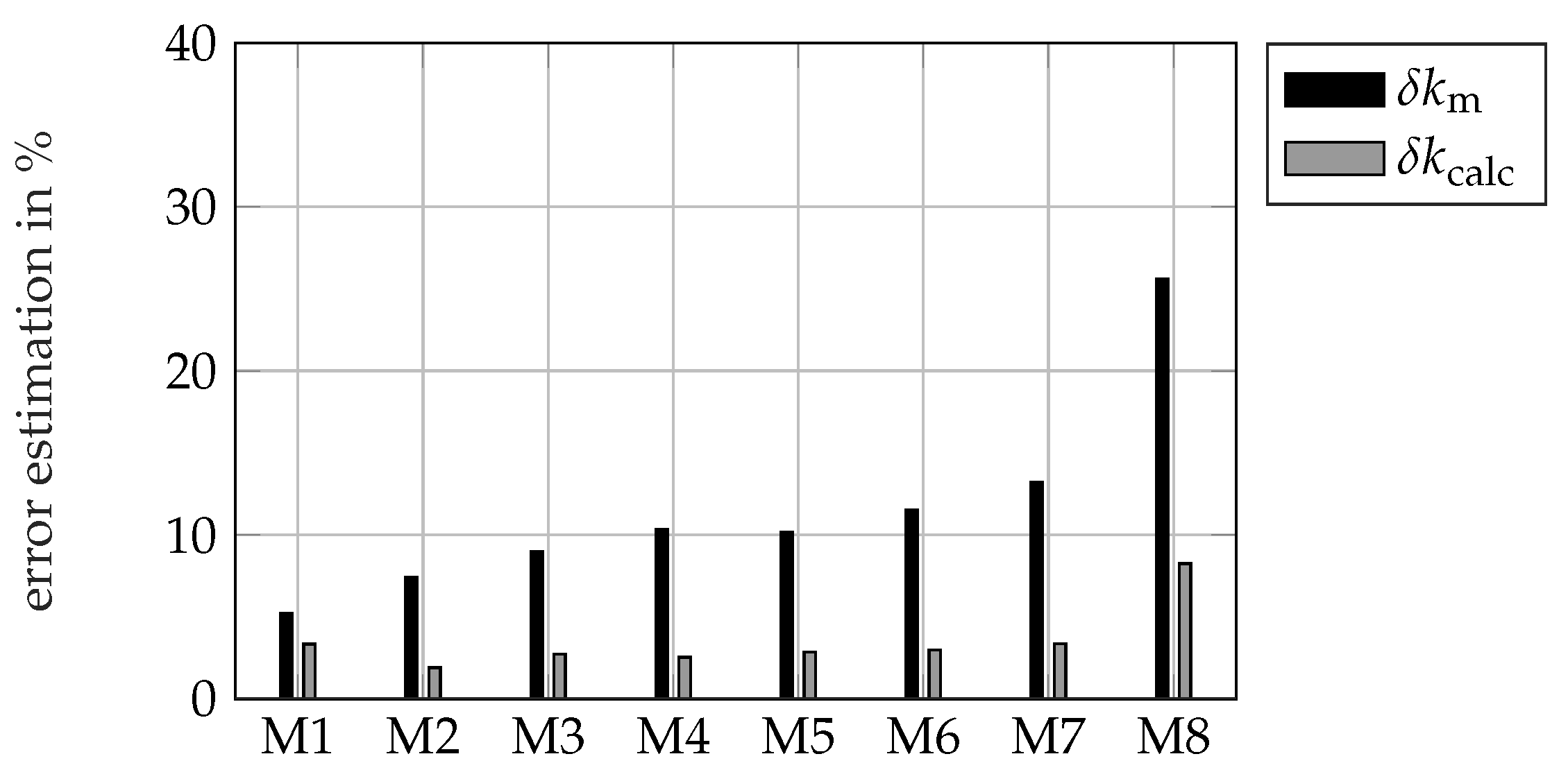
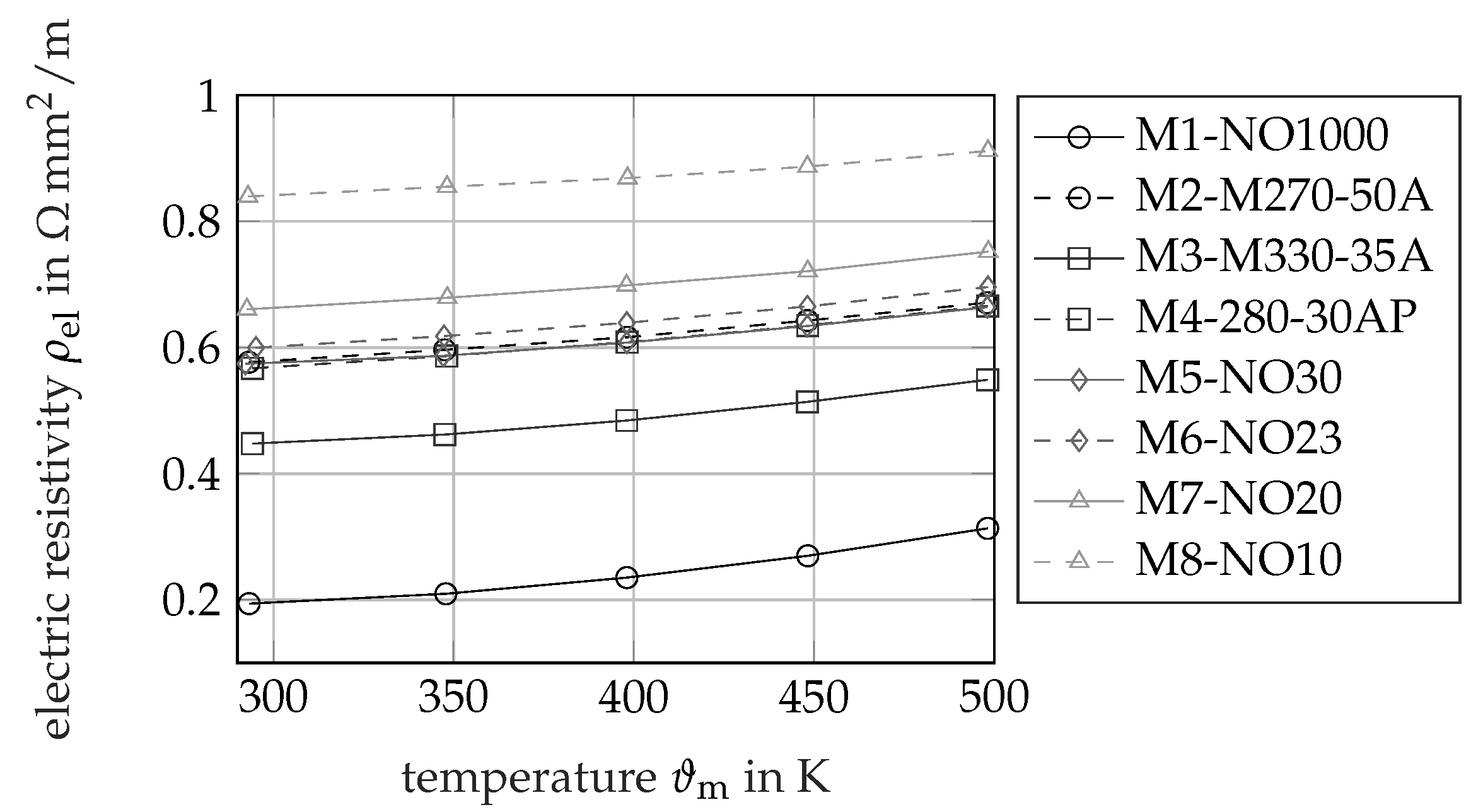
2.3. Measurements of the Temperature Dependent Electric Resistivity

Measurements of the electric resistivity are performed using the measurement setup as depicted in Figure 1. The setup is designed following the recommendations of the standard DIN EN IEC 60404-13 [14] on a smaller scale because the specimens are not available in the recommended size. Probes of 120   m m × 20   m m are used. In order to gain sufficient accuracy, an analysis of the measurement uncertainties is performed. The specimen is inserted into a measurement fixture and placed inside an oven. The electric resistivity ρ el ( ϑ ) is calculated with the following equation:
ρ el ( ϑ ) = U ( ϑ ) · d · w I · l .
A DC-current I between 0.2 A and 2 A is introduced into the sample using a FLUKE 5500A Multi-Product Calibrator [15]. The maximum measurement error of this current is given by Δ I = 0.64   m A in the manufacturer data sheet [15]. The voltage is measured with a separate device to improve the accuracy of the measurement. A HP 3458A Multimeter is used for this purpose. The maximum measured voltage during the procedure is around 20   m V . With an maximum measurement error of 16.4 ppm of the reading and 22 ppm of the measurement range, a maximum measurement error for the voltage of Δ U = 2.5   μ V is specified in the data sheet of the device [16]. Two measurement tips are placed on the probe for the voltage measurement. The distance between the measurement tips is equal to the measuring length l. The measuring length l as well as the width of the specimen w are measured using a digital caliper from Mitutoyo. The maximum measurement error of the measurement device is given with 0.02   m m . In order to include measurement errors that result from geometrical deviations, a total error estimation of Δ l = Δ w = 0.05   m m is included in the accuracy calculation. The measurement of the two values is repeated at least three times and the average value is calculated. The thickness of the sheet d is measured after removing the insulation, using an outside micrometer from Mitutoyo. The measurement is repeated six times and the average value is used. The coefficient of variation c v of the iterative geometrical measurement procedure is given in Table 2. c v is well below 1 % with one outlier of material M8 for the thickness measurement. The measurements show good precision.
The maximum measurement error of the micrometer is given with 0.001   m m . In order to account for geometric errors, a total measurement error estimation of Δ d = 0.01   m m for the thickness d is used for the accuracy evaluation. The measurement error estimation Δ ρ el is calculated at room temperature ϑ = 293   K using the following formula:
Δ ρ el ( ϑ ) = ( U ( ϑ ) + Δ U ) · ( d + Δ d ) · ( w + Δ w ) ( I Δ I ) · ( l Δ l ) ρ el ( ϑ ) .
The results of the accuracy study ( x = ρ el ) are depicted in table Table 3. A trend of increasing measurement errors with decreasing specimen thickness can be observed. One exception of this trend is the decreased accuracy of M1 in comparison to M2. This exception is caused by an increased influence of Δ U for this material. Due to the high thickness of this material, the resulting measured voltage U is relatively low at a comparable current I. For decreasing thickness, the error caused by the thickness d dominates the overall influence. For material M8 for instance, the measurement error of the thickness measurement Δ d causes about 10.6 % , while other influences only contribute by 1.1 % . Please note that this influence also could not have been changed utilizing the recommended setup in DIN EN IEC 60404-13 [14], as the thickness of the specimen would have a similar influence. The results of the measurement of the electric resistivity in dependency on the temperature ρ el ( ϑ ) are plotted in Figure 2. The results show a significant difference for the electric resistivity ρ el between the different materials. At first glance, the material d seems to influence the ρ el . This impression is not correct because the alloy components Si and Al are the primary influencing factors. As an example, M1 is the thickest selected material and has a very low silicon and aluminum content. Material M8 is the thinnest material with the highest silicon content. A plausibility check can be performed utilizing the ternary plot of the electric resistivity ρ el as a function of the silicon c w , Si and aluminum c w , Si and weight content published in [17]. The eight different materials are added to the plot in Figure 3 based on their silicon and aluminum content. The gained experimental results show very good agreement with this plot gained from the literature at room temperature.

3. Experimental Evaluation of the Thermal Conductivity

An indirect measurement technique is used for the evaluation of the thermal conductivity k m ( ϑ ) , i.e., the thermal diffusivity a ( ϑ ) is measured. The thermal conductivity of the measurement k m is calculated using the following formula:
k m ( ϑ ) = a ( ϑ ) · ρ ( ϑ ) · c p ( ϑ )
The procedure of evaluating the thermal diffusivity a ( ϑ ) , the mass density ρ ( ϑ ) , and the specific heat capacity c p ( ϑ ) is introduced in the following.

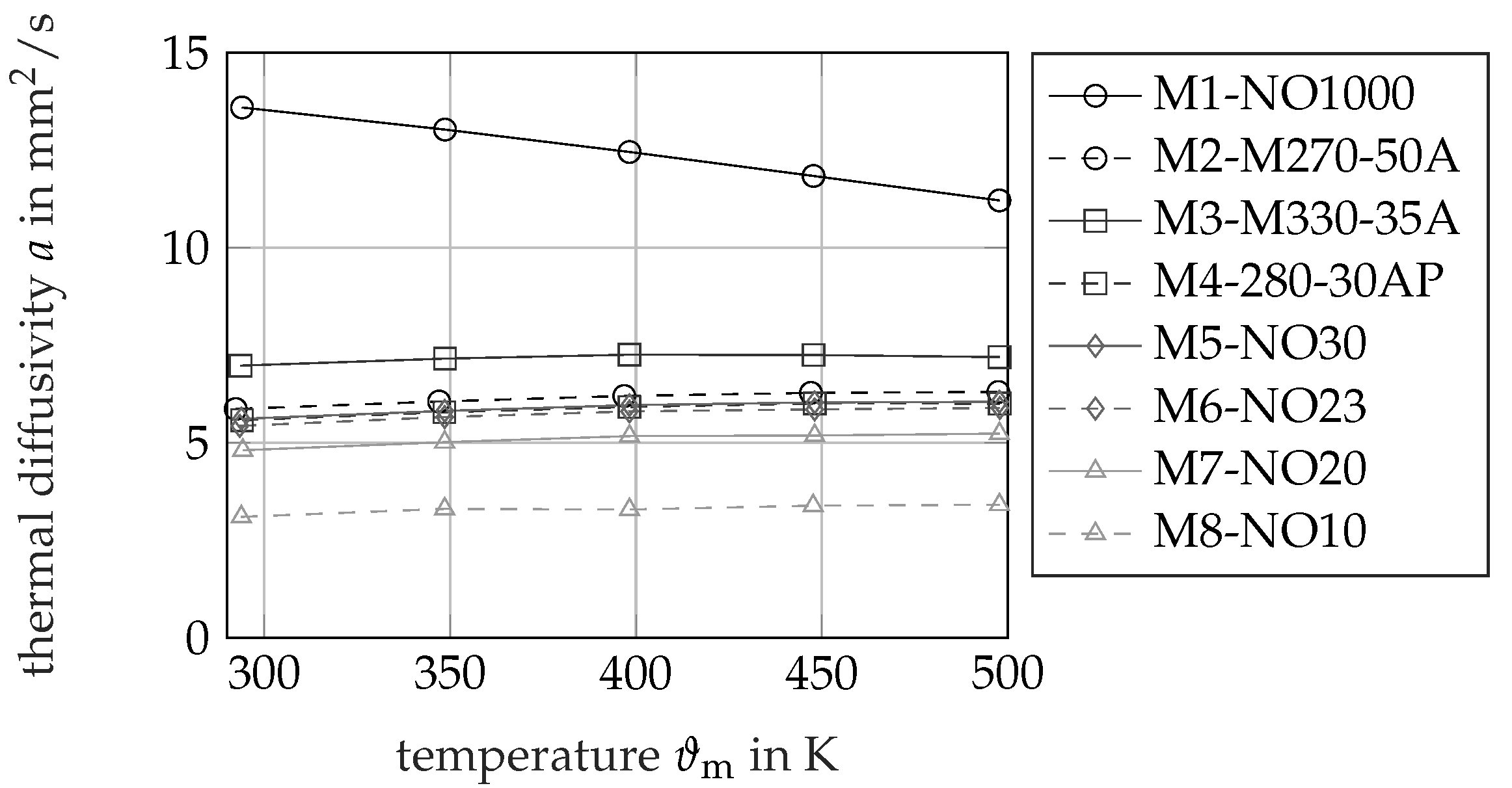
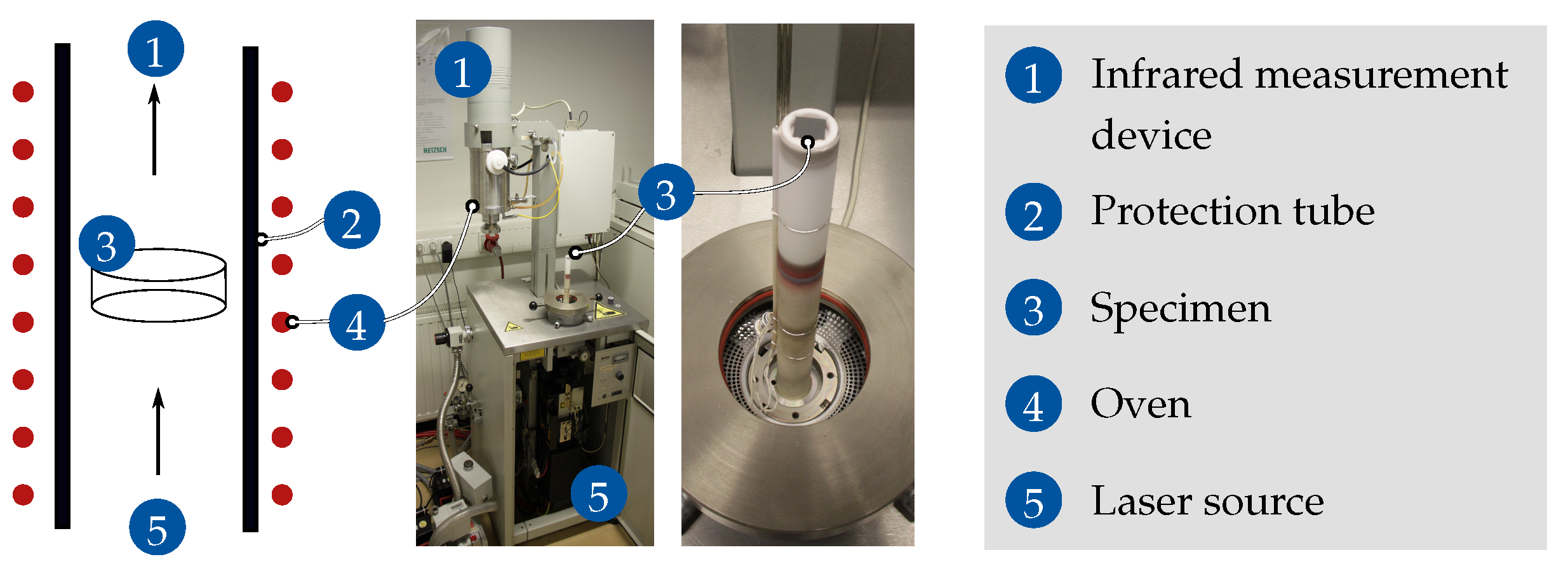
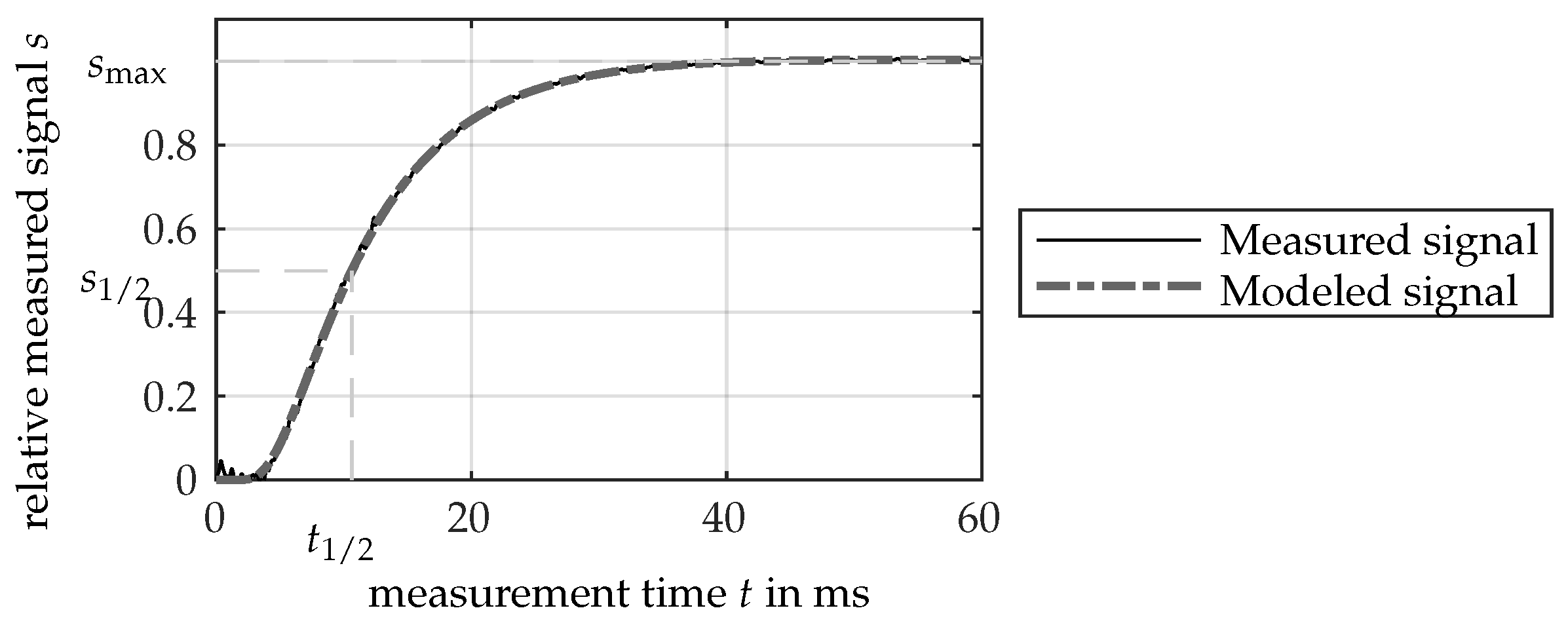
3.1. Measurements of the Thermal Diffusivity

The measurements of the thermal diffusivity are performed with a Netzsch LFA 427 measurement device. The samples are cut into specimens with a side length of 10   m m ± 0.1   m m . The insulation of the steel sheets is removed with sandpaper with a 500 grit. A thin graphite layer is added on the samples for improved absorption of the laser impulse. A schematic overview as well as some images of the measurement device are depicted in Figure 4. The specimen is inserted into the sample holder. The device is closed, and the sample is purged with argon as a protective gas. A laser pulse is shot at the specimen, and the temperature rise is measured on the back side using an indium antimonide (InSb) infrared detector. An exemplary measurement signal of material M1 at 348   K is depicted in Figure 5. Different models are available for the evaluation of the thermal diffusivity. The first approach is introduced by Parker [18]. The relative maximum signal s max = 1 is evaluated. The half time t 1 / 2 represents the time, when half s 1 / 2 of the maximum signal s max is reached. The half time is used to calculate the thermal diffusivity a according to [18]:
a = 0.1388 d 2 t 1 / 2 .
Parker assumes ideal conditions, such as an instantaneous energy pulse, adiabatic boundary conditions or constant material properties during the temperature rise. Several improvements of this model are performed. The losses on the front and rear end are added by Cowan [19]. Radial losses are added by Cape–Lehman [20]. Within this study, the standard model with a horizontal baseline correction of the NETZSCH Proteus Software Version 7.1.0. is used, i.e., an improved version of the Cape–Lehman formulation. A total of five temperatures are measured for each material, ranging from room temperature up to 498   K . At each temperature, at least six measurements are used for the calculation of the average value and the variation. The coefficient of variation of the thermal diffusivity measurements c v is given in Table 4.
The coefficient of variation is below 1.22 % for all materials, except material M8. Material M8 shows a maximum coefficient of variation of 2.7 % . These values indicate a good precision of the measurement. Please note that these values only consider the influence of the thermal diffusivity measurement procedure, i.e., the thickness is a constant value and not considered in Table 4. The measurement is repeated five times, and the average value is used for the measurements. For the measurement error estimation, the simplified Parker formula is used [18]. The general accuracy of the NETZSCH LFA is assumed to be ± 3 % for a 1   m m sample as given in the device data sheet [21]. This value is not included in the accuracy of different thickness measurements, as one constant value is being used during LFA measurements. The thickness is measured with a similar outside micrometer as utilized in the measurement of the electric resistivity with a maximum measurement error of 0.001   m m . A value of Δ d = 0.01   m m is used for the error estimation to include geometrical errors. The estimated error of the resulting thermal diffusivity Δ a is calculated as follows:
Δ a = 0.1388   ( d + Δ d ) 2 t 1 / 2 · x m
The value for x m is selected to be 1 % , as for this value, the measurement error of the 1 m m sample of M1 fits to the given data sheet value for the maximum measurement error of 3 % . The resulting estimated measurement errors according to Equation (3) for x = a are depicted in Table 5. A strong dependency on the thickness of the specimen is evaluated. The results of the thermal diffusivity measurement a are shown in Figure 6.
The thermal diffusivity a varies in a range from 3.1   m m 2 / s to 13.6   m m 2 / s . A significant difference between the values of the eight materials is visible. In particular, material M1 with a very low alloy content (see Table 1) and M8 with a very high alloy content stand out in the comparison. The thermal diffusivity of M1 is about 434 % larger than the thermal diffusivity of M8 at 298   K . The thermal diffusivity is expected to play a significant role in the calculation of the thermal conductivity (Equation (19)) and the maximum possible dissipated heat in the application.

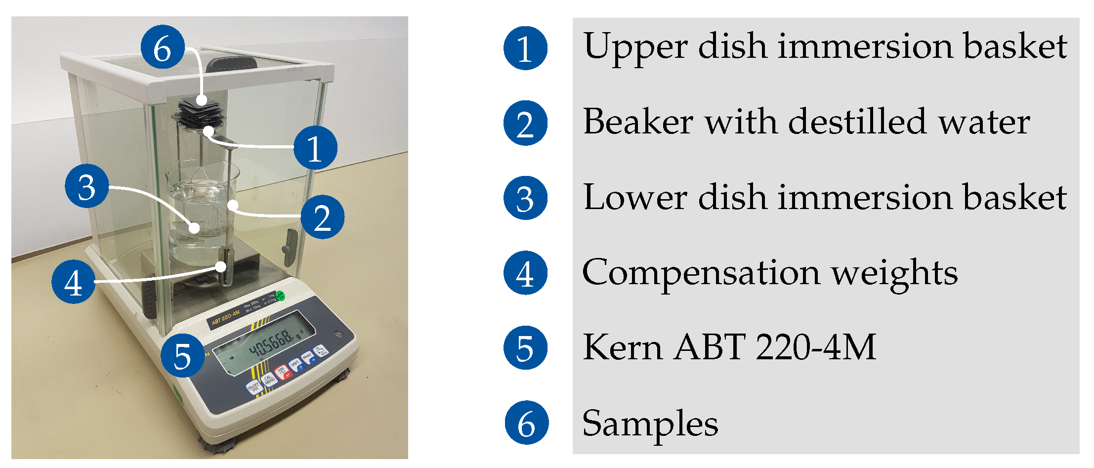
3.2. Measurements of the Density

Two different possibilities to measure the density of the sheets are studied and compared. The first methodology is a geometric-based method, utilizing the dimensions and the mass of the specimens. The LFA specimens are used for this purpose with the length l 10   m m , the width w 10   m m , and the thickness from d 0.1   m m up to d 1   m m . The measurement of the three values is repeated five times and an average value is calculated. Similar measurement equipment, as described in the measurements of the electric resistivity, is used for all three quantities. The estimation of the measurement error is Δ d = 0.01   m m and Δ l = Δ w = 0.05   m m . The weight m of the probe is measured using a Sartorius high precision balance with a maximum error of 0.1   m g . In order to account for possible dust or additional influences, a value of Δ m = 1   m g is used for the accuracy study.
ρ = m d · l · w
The error of the procedure can be estimated with the following:
Δ ρ = m + Δ m ( d Δ d ) · ( l Δ l ) · ( w Δ w )
The second methodology utilizes the principle of Archimedes. In this measurement technique, no exact cubic probe is necessary. A higher amount of pieces can be utilized to obtain a higher overall measured weight. The insulation of the material is removed by sandblasting. The density measurements are performed with an analytical balance Kern ABT 220-4M. The measurement error of the weight measurement is 0.1   m g . Multiple probes are cut into specimens that fit into the universal immersion basket of the balance. An overview of the measurement equipment is given in Figure 7. The distilled water, used as the reference fluid, is filled into a beaker. The temperature of the reference fluid ϑ 0 is measured, utilizing the thermometer included in the balance equipment. The density of the reference fluid is evaluated from a lookup table ρ 0 = f ( ϑ 0 ) . The error of the mass density of the reference fluid is estimated by a 5   K -deviation in the temperature measurement as follows:
Δ ρ 0 ( ϑ ) = ρ 0 ( ϑ ) ρ 0 ( ϑ + 5 K )
The first measurement is performed with the specimens placed onto an upper sample dish of the immersion basket. The amount of samples is adapted to obtain a total weight of approximately m A 40   g . The measured value of m A is the result of the difference between the buoyancy force of the air and the weight force of the specimen:
m A = ( ρ ρ air ) · V ,
with the volume of the specimen V, and the density of air ρ air . The influence of the air buoyancy force is neglected in the calculation. An additional factor is considered in the error estimation of Δ m A :
Δ m A = ρ air ρ · m A + 1   m g
The measurement is repeated with the samples placed on the lower dish of the immersion basket. The measured weight m B is equal to the following:
m B = ( ρ ρ 0 ) · V .
The estimated error of the measurement of m B is assumed to be equal to Δ m B = 1   m g . The combination of Equations (25) and (27) under neglection of the air buoyancy force gives the equation to calculate the mass density ρ of the specimen.
ρ = m A m A m B ρ 0
A worst-case estimation for the measurement error of the density ρ is performed with the following:
Δ ρ = m A + Δ m A ( m A Δ m A m B Δ m B ) · ( ρ 0 + Δ ρ 0 ) ρ
The entire measurement procedure is repeated three times. After each measurement in the water reference, the samples are dried. A thin rust film develops within seconds and is removed by sandblasting. All values are reevaluated, including the masses m A and m B , as the repeated sandblasting also removes some of the material. An average value of the three measurements is calculated.
The results of the measurements as well as the error estimation according to the calculation of Equation (3) for x = ρ are depicted in Table 6. The coefficient of variation c v for the measured values is added. c v of the geometrical values l , d and w shows values below 1.1 % for most of the values. Only the thickness measurements show larger values with 2.5 % for M8 and 1.86 % for M6. The coefficient of variation for the Archimedes principle shows small values below 0.13 % for all measured materials. The precision of the Archimedes principle is significantly improved in comparison to the geometrical principle. The accuracy of the geometrical principle is mainly driven by the estimated error of the thickness measurement Δ d , which leads to high error estimations for the thin sheets. The error estimation model gives a minimal value of 2.2 % for the thickness material M1 and 14.7 % for the thinnest material. The estimated error of the Archimedes principle with values around 0.2 % is very low and almost equal for all probes. The accuracy is independent from the thickness of the probe. The variation for the three measurement repetitions of the Archimedes principle varies between 0.01 % and 0.13 % . This value is lower than the predicted values for the measurement error δ ρ in Table 6. This observation confirms the good precision of the measurement and confirms the estimation of the measurement accuracy being the critical value. The measured density utilizing the geometrical principle is lower than the density evaluated by the Archimedes principle between 3.2 % and 4.7 % . It is interesting to note that the values are all lower and not spread around the exact values of the Archimedes principle. The difference between the results shows the lowest value for Material M1, which confirms the trend indicated by the accuracy study. Additionally, the value of 3.2 % is larger than the predicted error of 2.2 % as a sum of the two error estimations. There are obviously some additional systematic errors present. Issues with air bubbles in the Archimedes measurement do not seem to be present, as the variation coefficient of the measurement is low. Air bubbles in the second measurement step would decrease m B , which leads to an underestimation of the density ρ . This is not the case, because the results of the Archimedes principle are all larger than those of the geometrical probes. A possible explanation for the effect is the cuboid model that is used for the estimation of the volume in the geometric approach. The measured values are the outer dimensions. Irregularities and roughness could lead to a real volume that is lower. This would cause lower values of the density ρ . The temperature dependency is estimated, using a thermal expansion coefficient of α th = 11.8 × 10 6 / K .
ρ ( ϑ ) = ρ · 1 1 + 3 · α th · ( ϑ ϑ 0 ) ,
with the measurement temperature as the reference temperature ϑ 0 .
The density ρ varies in a range from 7479 kg/m to 7834 kg/m. The value for material M1 is only 5 % larger than the value of M8 at 298   K . The mass density is expected to play a minor role for the differences in the thermal conductivities of the materials, according to Equation (19) and the maximum possible dissipated heat in the application. In the case of a study with fewer accuracy requirements, an average value of the expected density could be used with a maximum error of the indicated 5 % .

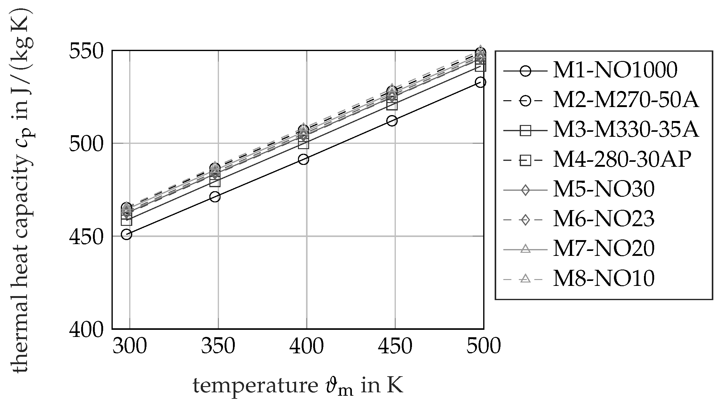
3.3. Evaluation of the Thermal Heat Capacity

The influence of alloy components on the specific thermal heat capacity c p can be evaluated utilizing the Kopp–Neumann law. The weight content of each alloy c w i as well as the specific heat capacity of each alloy component c p i needs to be known for this law:
c p = i c w i · c p i ,
Both requirements are fulfilled for this study. Temperature-dependent measurement data of the specific heat capacities are available in the literature for silicon [22], aluminum [23], and pure iron [24]. Within this input data, the temperature dependency is considered as used in [25]:
c p ( ϑ ) = i c w i · c p i ( ϑ )
The resulting heat capacities in dependency of the temperature are depicted in Figure 8. The Kopp–Neumann law is, strictly speaking, only valid for composites but the comparison of measured heat capacities of Fe-based alloys with the Kopp–Neumann law can be found in the literature, such as [26]. Further, the difference of the calculated heat capacity of the eight materials shows minor influence on the later thermal conductivity. This can be illustrated with the maximum deviation of the values at room temperature. The c p of M1 deviates from the M8 value at room temperature by 3.6 % . The thermal diffusivity a of M1 is 334 % larger than the value of M8 at room temperature. For further validation and estimation of the errors, the calculated values of the heat capacity based on Equation (31) are compared to the results evaluated from the commercial software JMatPro Version 8. The comparison is performed for pure iron and Materials M7 and M8, which are the materials with the highest Al and Si content, respectively. The maximum deviation between the two approaches is around 1 % . For the error estimation study, a value of δ c p rel = 2 % is used for all materials.
Due to the small differences between c p of the different materials, only a minor influence on the difference of the thermal conductivities of the materials, according to Equation (19), is expected. A minor influence on the maximum dissipated heat is expected. The value varies between 451   J / k g / K for M1 and 465   J / k g / K for M8. In the case of a study with fewer accuracy requirements, an average value of the expected heat capacity could be used with a maximum error of the indicated 3.6 % .

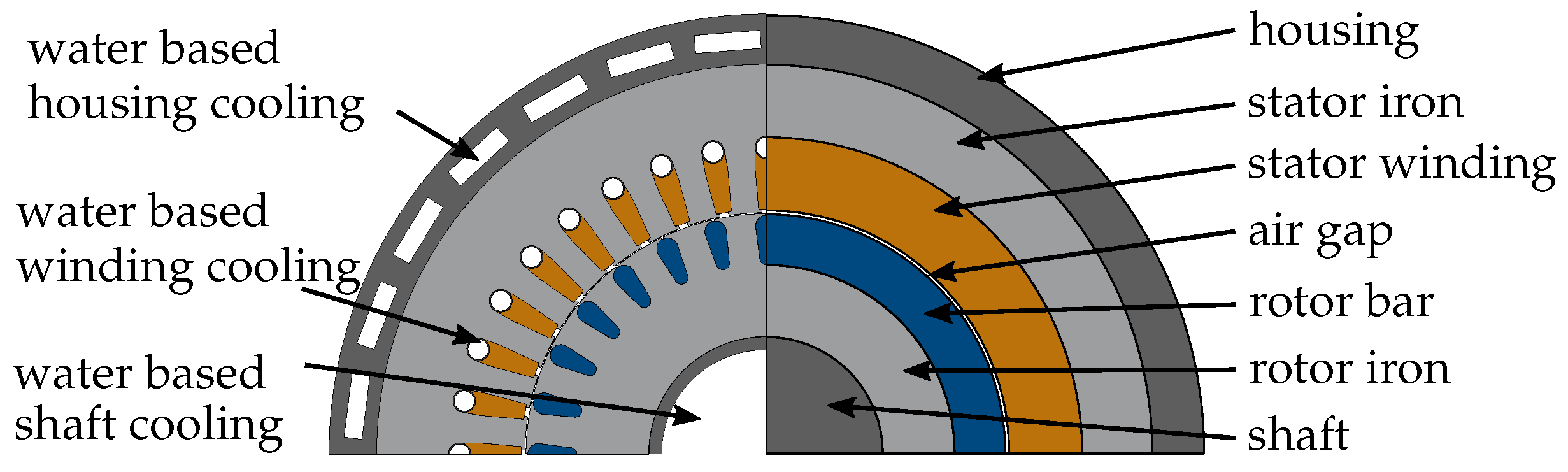
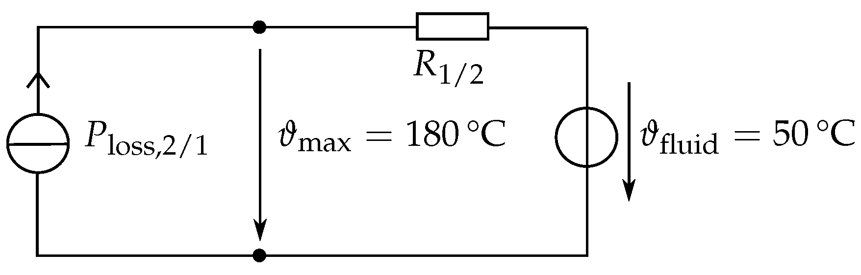
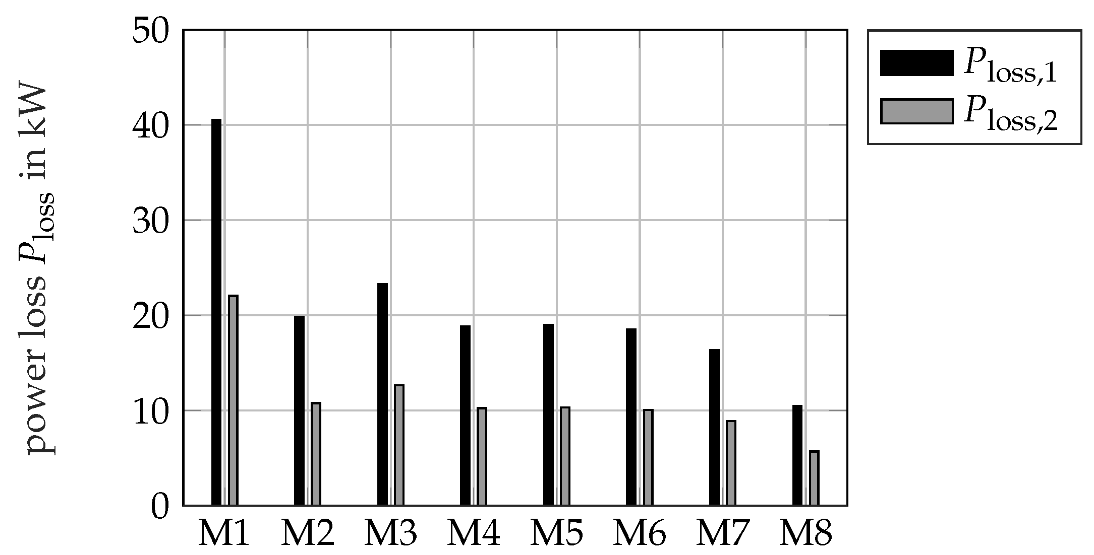
4. Simplified Case Study

The influence of the thermal conductivity k of the different materials should be studied in a simplified case study. This investigation is performed from a thermal perspective. The used reference design is an induction machine for a commercial truck traction application [5]. The following question is in the focus of the study:
How much loss power can be extracted from the electric machine in dependency of the used soft magnetic material?
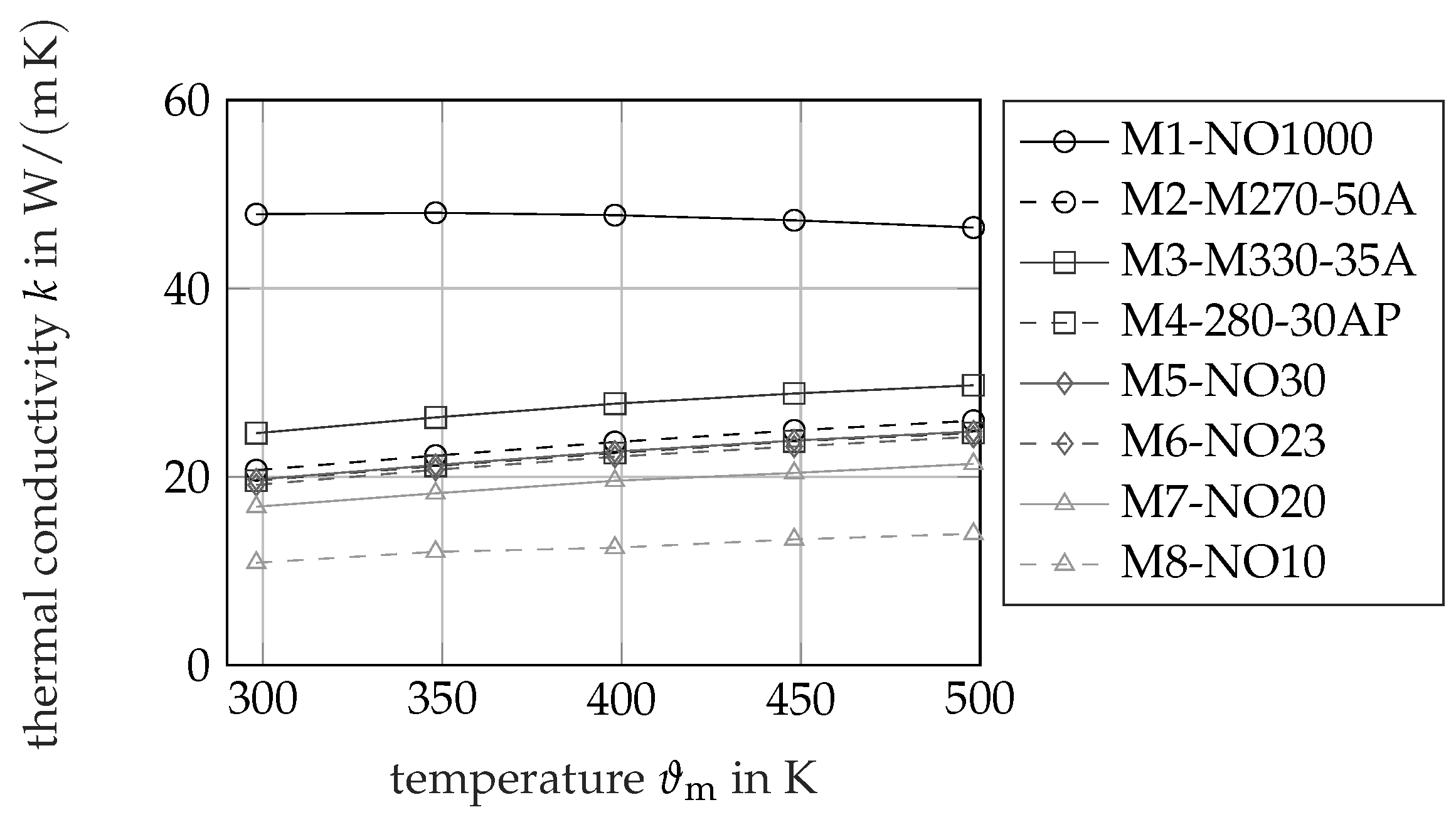
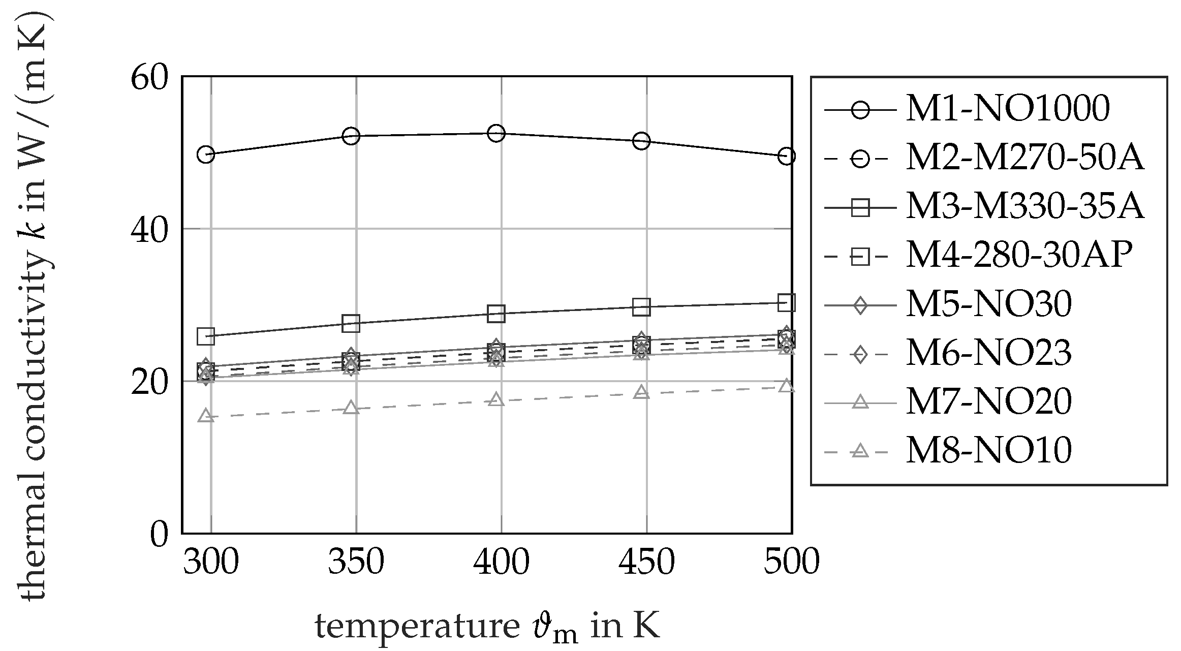
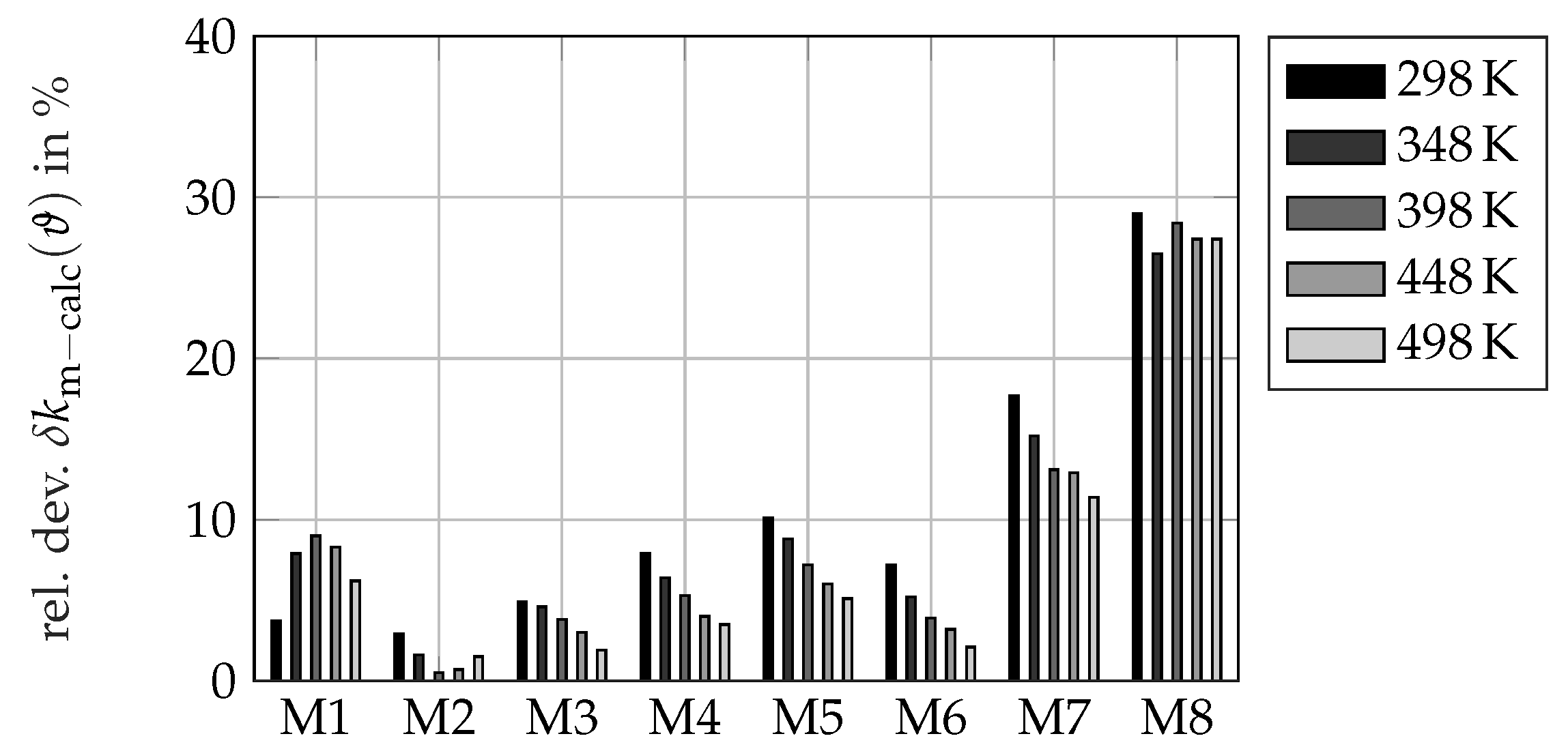
Please note that this study does not aim to use a highly accurate thermal model of the machine. The model is kept as simple as possible to understand the fundamental correlations of the material choice. The following assumptions and boundary conditions are made: the rotor and stator of the machine are separated by an ideal thermal insulator, i.e., no heat is transferred through the air gap. The stator is equipped with a housing cooling. The rotor is equipped with a rotor shaft cooling. The stator notch cooling, as found in [5], is not considered. The geometry is simplified by a cylindrical shell model as depicted in Figure 9. The height of the stator yoke and the height of the rotor yoke are kept constant, i.e., the heat transfer path through this part of the lamination is kept constant, and the influence of the teeth is neglected. The model is two-dimensional, i.e., the influence of heat extraction in end windings, bearings and bearing shields is neglected. All stator losses are introduced in the shell of the stator winding, and all rotor losses are introduced in the shell of the rotor bar. The heat conduction of the stator winding shell and the rotor bar shell is infinite. All thermal interface resistances are neglected. The housing and the shaft have the same temperature as the cooling fluid ϑ fluid = 50   C , i.e., the thermal resistance between the lamination and the housing/shaft, the convectional resistance between wall and fluid, and the heating up of the fluid are neglected. The bending of the shells is neglected, i.e., the shells are modeled as flat plates, utilizing the average diameter of the shell ( d out + d i ) / 2 . The thermal resistance of the stator R 1 and rotor R 2 iron are calculated as follows:
R 1 / 2 = d out , 1 / 2 d i , 1 / 2 k m · π · ( d out , 1 / 2 + d i , 1 / 2 ) · l i ,
with the outer and inner diameters d out 1 = 282   m m ;   d out 2 = 168   m m ;   d i 1 = 214   m m and d i 2 = 100   m m , the active length of the lamination l i = 285   m m , and the evaluated thermal conductivity of the measurements k m . The studied operational point is under steady-state behavior. The two thermal Lumped Parameter Thermal Network (LPTN) circuits are depicted in Figure 10. The maximum allowed temperature of stator winding and rotor bar is ϑ max = 180   C . The maximum power loss P loss in the steady-state operation that can be extracted from the rotor or the stator is calculated as follows:
P loss = ϑ max ϑ fluid R 1 / 2 ( ϑ avg ) ,
with the average temperature of the stator or rotor iron ϑ avg = ( ϑ max + ϑ fluid ) / 2 .

5. Results

The thermal conductivity of the measurement approach k m ( ϑ ) is calculated utilizing Equation (19). The results of the more accurate Archimedes principle are used for the density values. The results of the measurement procedure are depicted in Figure 11. The results of the analytical calculation based on Equations (9) and (16) are given in Figure 12. Material M1 has the highest thermal conductivity, while M8 has the lowest thermal conductivity in both approaches. In the measurement approach, the difference in the thermal conductivity k m mainly results from the different values of the thermal diffusivity measurements a as shown in Figure 6. The differences in the density ρ and the thermal heat capacity c p seem to have a minor impact on the difference of the thermal conductivity k m .
A comparison between the measurement and the analytical approach is performed. The relative difference between k calc ( ϑ ) and k m ( ϑ ) is calculated as follows:
δ k m calc ( ϑ ) = k calc ( ϑ ) k m ( ϑ ) k calc ( ϑ )
The value of this difference is plotted in Figure 13. The results of the analytical and the experimental approach show very good agreement for most of the materials. Materials M1 up to M6 show differences smaller than 10 % for the entire temperature range. The differences for ϑ = θ D are significantly smaller. Materials M7 and M8 show higher differences, below 18 % for material M7 and below 30 % for material M8.
A possible reason for the deviation can be evaluated by the analysis of the overall estimated error of the two different procedures. The previously examined errors are multiplied to gain the overall error estimation of the measurement.
δ k m = δ ρ · δ a · δ c p
For the analytical approach, solely the influence of the measurement of the electric resistivity δ ρ el is considered.
δ k calc ( ϑ ) = k calc ( ϑ , ρ el · ( 1 δ ρ el ) ) k calc ( ϑ , ρ el ) 1
The value is evaluated at ϑ = 398   K . The results of the accuracy studies δ k m and δ k calc are depicted in Figure 14. The accuracy study shows a clear dependency of the measurement results on the material thickness d. In particular, the estimated measurement errors of the thermal diffusivity δ a has a squared dependency on the material thickness d. The influence of the thickness is also visible for the estimated errors of the electric resistivity measurement δ ρ el , where the estimated thickness error has a linear influence. This linear influence shows some impact on the accuracy of the calculated thermal conductivity value k calc . The deviation between the measurement and calculation results δ k m calc ( ϑ ) shows a similar trend as the estimated errors δ k m and δ k calc . An allocation of the two effects is very likely, but not absolute clearly justifiable in the eyes of the authors. Material M8 is by far the thinnest material d 0.1   m m but also has by far the highest silicon content. It is also possible that the used formula has some inaccuracies in predicting such high silicon contents. Due to the estimated measurement errors for M8, a clear separation is not possible. The second material with higher deviations between measurement and calculation is M7. It is the second thinnest material, i.e., the nominal thickness is d 0.2   m m . M7 has a significantly lower silicon content than M8, but the highest aluminum content. The alloying contents are close to those of M2 that show the lowest deviation of all materials between the measurement and the analytical approach. This indicates that the formula is accurate for the given alloys, and the differences of M7 occur due to the measurement errors of the material or some other structural influences that are not considered in the given formula.
The influence of the alloys on the phonon and electron thermal conductivity can be analyzed based on the introduced formula. The evaluation is performed at ϑ = 398   K . The phonon thermal conductivity k p deviates from 6.8   W / ( m   K ) for M8 up to 15.7   W / ( m   K ) for M1. The electron thermal conductivity k e deviates from 8.5   W / ( m   K ) for M8 up to 34.0   W / ( m   K ) for M1. Both values show significant deviations, whereas the electron thermal conductivity has the higher impact on the overall value. The influence is limited to the electron–impurity scatter W e i according to Equation (13) and the phonon–impurity scatter W p i according to Equation (8). Other scattering processes are not influenced according to the used formula.
The results of the simplified case study are depicted in Figure 15. Material M1 shows the most preferable thermal properties. With this material, a maximum of 41   k W stator losses and 22   k W rotor losses could be extracted from the motor in the steady-state operation. With material M8, only 10   k W stator losses and 6   k W rotor losses would be allowed to ensure steady-state operation. It is well visible that all materials with high aluminum and silicon content show significant disadvantages regarding their capability for heat extraction. Please note that this estimation is based on some significant simplifications.

6. Discussion

An analytical as well as an experimental approach are performed to study the influence of the silicon and aluminum content of soft magnetic materials on their thermal conductivity. The two approaches show very good agreement for a majority of the studied materials and analyzed temperatures. The thickness of the probes is identified as a crucial factor for the accuracy of the measurements. The validity of the experimental values of the thin samples M8 is restricted. The results indicate a significant influence of the alloying contents on the thermal conductivity of the materials. A simplified case study is performed. The maximum possible heat that can be extracted from the rotor and stator of a reference induction machine varies by a factor of up to four for the different materials. It is obvious that this factor should be considered in the design process of high power density traction drives in the case that a main heat dissipation path is realized over the lamination of the machine.
A measurement of a thicker material with a very high silicon content would be helpful to further identify whether the introduced formula needs to be adjusted for such alloys. In a real application, additional thermal resistances would be present that reduce the calculated impact on the thermal dissipation. The different materials, of course, also influence the magnetization behavior and the produced losses in the material. The selection of the material should consider all these aspects. Detailed measurements of the loss behavior of the studied materials, a thermal model of the studied motor, a test bench evaluation of the entire motor and a simulation study including thermal, loss and magnetization aspects is on the way.

Author Contributions

Conceptualization, B.G, A.R., N.L. and K.H.; methodology, B.G. and A.R.; software, B.G. and A.R.; validation, B.G., A.R. and N.L.; formal analysis, B.G. and A.R.; writing—original draft preparation, B.G.; writing—review and editing, B.G., A.R., N.L. and K.H.; visualization, B.G. and A.R.; supervision, K.H.; project administration, K.H.; funding acquisition, K.H. All authors have read and agreed to the published version of the manuscript.

Funding

This research and development project “Concept-ELV2(01MY17002B)” is funded by the German Federal Ministry for Economic Affairs and Enegry (BMWi). The authors are grateful to the BMWi for the financing of this collaboration and who are responsible for the contents of this publication.

Institutional Review Board Statement

Not applicable.

Informed Consent Statement

Not applicable.

Acknowledgments

We want to thank the Institute for Materials Applications in Mechanical Engineering (iwm) of RWTH Aachen University and Netzsch Gerätebau GmbH for the excellent consultation and discussion within the project.

Conflicts of Interest

The authors declare no conflict of interest. The funders had no role in the design of the study; in the collection, analyses, or interpretation of data; in the writing of the manuscript, or in the decision to publish the results.

Abbreviations

The following abbreviations are used in this manuscript:
Acr.Acronym
AlAluminum
IMInduction Motor
InSbIndium Antimonide
LFALaser Flash Analysis
LPTNLumped Parameter Thermal Network
SISilicon

References

  1. Ruf, A.; Steentjes, S.; von Pfingsten, G.; Grosse, T.; Hameyer, K. Requirements on Soft Magnetic Materials for Electric Traction Motors. In Proceedings of the 7th international Conference on Magnetism and Metallurgy (WMM), Rome, Italy, 13–15 June 2016; pp. 111–128. [Google Scholar]
  2. Leuning, N.; Pauli, F.; Hameyer, K. Most appropriate soft magnetic material choice with consideration of structural material parameters for electrical machines. In Proceedings of the 8th International Conference on Magnetism and Metallurgy (WMM), Dresden, Germany, 12–14 June 2018; Universitätsverlag: Freiberg, Germany, 2018. [Google Scholar]
  3. Staton, D.; Boglietti, A.; Cavagnino, A. Solving the More Difficult Aspects of Electric Motor Thermal Analysis in Small and Medium Size Industrial Induction Motors. IEEE Trans. Energy Convers. 2005, 20, 620–628. [Google Scholar] [CrossRef] [Green Version]
  4. Groschup, B.; Nell, M.; Pauli, F.; Hameyer, K. Characteristic Thermal Parameters in Electric Motors: Comparison between Induction- and Permanent Magnet Excited Machine. IEEE Trans. Energy Convers. 2021, 36, 2239–2248. [Google Scholar] [CrossRef]
  5. Köller, S.; Uerlich, R.; Westphal, C.; Franck, M. Design of an Electric Drive Axle for a Heavy Truck. ATZ Heavyduty Worldw. 2021, 14, 20–25. [Google Scholar]
  6. JCGM. International Vocabulary of Metrology—Basic and General Concepts and Assocciated Terms (VIM), 3rd ed.; JCGM: Sevres, France, 2012. [Google Scholar]
  7. Klemens, P.G.; Williams, R.K. Thermal conductivity of metals and alloys. J. Appl. Phys. 1986, 31, 197–215. [Google Scholar]
  8. Wang, G.; Li, Y. Effects of alloying elements and temperature on thermal conductivity of ferrite. J. Appl. Phys. 2019, 126, 125118.1–125118.9. [Google Scholar] [CrossRef]
  9. Herbstein, F.H.; Smuts, J. Determination of Debye temperature of alpha-iron by X-ray diffraction. Philos. Mag. 1963, 8, 367–385. [Google Scholar] [CrossRef]
  10. Williams, R.K.; Yarbrough, D.W.; Masey, J.W.; Holder, T.K.; Graves, R.S. Experimental determination of the phonon and electron components of the thermal conductivity of bcc iron. J. Phys. Chem. Ref. Data 1981, 52, 5167–5175. [Google Scholar] [CrossRef]
  11. Williams, R.K.; Graves, R.S.; McElroy, D.L. Thermal and electrical conductivities of an improved 9 Cr-1 Mo steel from 360 to 1000 K. Int. J. Thermophys. 1984, 5, 301–313. [Google Scholar] [CrossRef]
  12. Julian, C.L. Theory of Heat Conduction in Rare-Gas Crystals. Phys. Rev. 1965, 137, A128–A137. [Google Scholar] [CrossRef]
  13. Bäcklund, N.G. An experimental investigation of the electrical and thermal conductivity of iron and some dilute iron alloys at temperatures above 100 °K. J. Phys. Chem. Solids 1961, 20, 1–16. [Google Scholar] [CrossRef]
  14. DIN German Institute for Standardization. Magnetic Materials—Part 3: Methods of Measurement of the Magnetic Properties of Electrical Steel Strip and Sheet by Means of a Single Sheet Tester (IEC 60404-3:1992 + A1:2002 + A2:2009); Beuth Verlag GmbH: Berlin, Germany, 2010. [Google Scholar]
  15. Corporation Fluke. Datasheet: Service Manual 5500A Multi-Product Calibrator; Fluke Corporation: Everett, WA, USA, 1995. [Google Scholar]
  16. Hewlett-Packard Company (HP). Datasheet: 3458A Multimeter Operating, Programming and Configuration; Manual, Hewlett-Packard Company (HP): Palo Alto, CA, USA, 1988. [Google Scholar]
  17. Wijn, H.P.J. Magnetic Alloys for Technical Applications. Soft Magnetic Alloys, Invar and Elinvar Alloys; Springer: Berlin/Heidelberg, Germany, 1994; Volume 19i1. [Google Scholar] [CrossRef]
  18. Parker, W.J.; Jenkins, R.J.; Butler, C.P.; Abbott, G.L. Flash Method of Determining Thermal Diffusivity, Heat Capacity, and Thermal Conductivity. J. Appl. Phys. 1961, 32, 1679–1684. [Google Scholar] [CrossRef]
  19. Cowan, R.D. Pulse Method of Measuring Thermal Diffusivity at High Temperatures. J. Appl. Phys. 1963, 34, 926–927. [Google Scholar] [CrossRef]
  20. Cape, J.A.; Lehman, G.W. Temperature and Finite Pulse—Time Effects in the Flash Method for Measuring Thermal Diffusivity. J. Appl. Phys. 1963, 34, 1909–1913. [Google Scholar] [CrossRef]
  21. NETZSCH. Laser Flash Apparatus LFA 427: Brochure; Netzsch-Gerätebau GmbH: Seib, Germany, 2021. [Google Scholar]
  22. Desai, P.D. Thermodynamic Properties of Iron and Silicon. J. Phys. Chem. Ref. Data 1986, 15, 967–983. [Google Scholar] [CrossRef]
  23. Chao, J.; Phillips, E.W.; Sinke, G.C.; Hu, A.T.; Prophet, H.; Syverud, A.N.; Karris, G.C.; Wollert, S.K. JANAF Thermochemical Tables Addendum; U.S. Department of Commerce: Washington, DC, USA, 1966.
  24. Chase, M.W.; Curnutt, J.L.; Downey, J.R.; McDonald, R.A.; Syverud, A.N.; Valenzuela, E.A. JANAF Thermochemical Tables, 1982 Supplement. J. Phys. Chem. Ref. Data 1982, 11, 695–940. [Google Scholar] [CrossRef] [Green Version]
  25. Novikov, V.V. Debye–Einstein model and anomalies of heat capacity temperature dependences of solid solutions at low temperatures. J. Therm. Anal. Calorim. 2019, 138, 265–272. [Google Scholar] [CrossRef]
  26. Hafenstein, S.; Werner, E.; Wilzer, J.; Theisen, W.; Weber, S.; Sunderkötter, C.; Bachmann, M. Influence of Temperature and Tempering Conditions on Thermal Conductivity of Hot Work Tool Steels for Hot Stamping Applications. Steel Res. Int. 2015, 86, 1628–1635. [Google Scholar] [CrossRef]
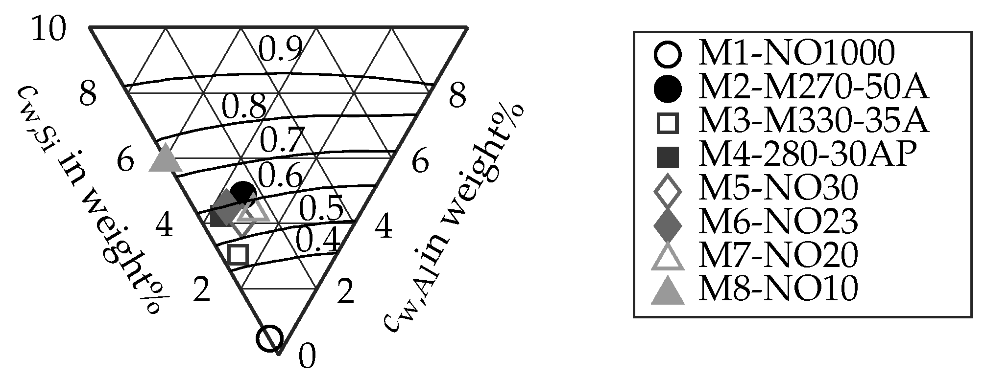
Figure 1. Measurement setup for the electric resistivity.
Energies 14 05310 g001
Figure 2. Results of the electric resistivity measurements ρ el ( ϑ ) .
Energies 14 05310 g002
Figure 3. Theoretical values for the electric resistivity ρ el ( ϑ = 298   K ) in Ω   m m 2 / m based on the silicon and aluminum content (Source: Data from [17]).
Energies 14 05310 g003
Figure 4. Measurement setup for the thermal diffusivity.
Energies 14 05310 g004
Figure 5. Exemplary measurement signal of material M1 at 348   K .
Energies 14 05310 g005
Figure 6. Results of the thermal diffusivity measurements a ( ϑ ) .
Energies 14 05310 g006
Figure 7. Analytical balance Kern ABT 220-4M with universal immersion basket.
Energies 14 05310 g007
Figure 8. Results of the calculation of the thermal heat capacity c p ( ϑ ) .
Energies 14 05310 g008
Figure 9. Real geometry (left) and simplified thermal shell model of the studied machine (right).
Energies 14 05310 g009
Figure 10. Lptn model of the simplified case study for the stator and the rotor.
Energies 14 05310 g010
Figure 11. Results of the measurements of the thermal conductivity k m .
Energies 14 05310 g011
Figure 12. Results of the calculation of the thermal conductivity k calc .
Energies 14 05310 g012
Figure 13. Relative difference between thermal conductivites gained from measurement and analytical formula δ k m calc ( ϑ ) .
Energies 14 05310 g013
Figure 14. Relative predicted error of the measured values of the thermal conductivity δ k .
Energies 14 05310 g014
Figure 15. Lptn model of the simplified case study for the stator and the rotor.
Energies 14 05310 g015
Table 1. Alloy weight content and nominal thickness of studied materials.
NameAcr.Si
in  %
Al
in  %
d
in mm
NO1000M10.470.031
M270-50AM23.381.490.5
M330-35AM32.60.440.35
280-30APM43.640.590.30
NO30M531.0670.30
NO23M63.640.870.23
NO20M72.911.570.20
NO10M8600.10
Table 2. Coefficient of variation c v for measurements of geometrical values in %.
Material cv ( l ) cv ( w ) cv ( d )
M1-NO10000.290.040.08
M2-M270-50A0.090.041.00
M3-M330-35A0.410.020.91
M4-280-30AP0.090.030.63
M5-NO300.190.030.85
M6-NO230.060.080.54
M7-NO200.300.040.72
M8-NO100.300.061.28
Table 3. Estimated measurement error δ ρ el ( ϑ = 293   K ) in % .
Material δ ρ el Material δ ρ el Material δ ρ el
M1-NO10004.3M2-M270-50A2.9M3-M330-35A3.9
M4-280-30AP3.8M5-NO304.3M6-NO234.5
M7-NO205.3M8-NO1011.7
Table 4. Coefficient of variation c v for measurements of thermal diffusivity a in %.
Material ϑ = 293 K ϑ = 348 K ϑ = 398 K ϑ = 448 K ϑ = 498 K
M1-NO10001.130.800.621.220.52
M2-M270-50A0.900.330.210.190.21
M3-M330-35A0.660.450.400.510.40
M4-280-30AP0.410.610.440.520.72
M5-NO300.610.460.600.500.36
M6-NO230.630.720.590.700.70
M7-NO200.980.740.560.810.94
M8-NO101.611.242.651.530.76
Table 5. Estimated measurement error of the thermal diffusivity measurement x = a in %.
Material δ ρ el Material δ ρ el Material δ ρ el
M1-NO10003.0M2-M270-50A5.2M3-M330-35A6.8
M4-280-30AP8.1M5-NO308.0M6-NO239.3
M7-NO2011.0M8-NO1023.4
Table 6. Measurement results and error estimation of the density measurement at ϑ 293   K .
Geometrical PrincipleArchimedes Principle
Material cv ( l )
in %
cv ( w )
in %
cv ( d )
in %
ρ
in kg/m3
δ ρ
in %
cv ( ρ )
in %
ρ
in kg/m3
δ ρ
in %
M1-NO10000.150.050.2575812.20.1378340.21
M2-M270-50A0.020.061.0572883.40.0275530.21
M3-M330-35A0.060.070.5773984.40.1376780.20
M4-280-30AP0.031.100.3872225.20.0675790.21
M5-NO300.080.070.4573025.10.0475650.21
M6-NO230.160.021.8672715.90.0175760.20
M7-NO200.100.020.5671626.90.0275030.24
M8-NO100.070.202.50696414.70.1274790.22
Publisher’s Note: MDPI stays neutral with regard to jurisdictional claims in published maps and institutional affiliations.

