Abstract
This research presents a validation methodology for computational fluid dynamics (CFD) assessments of rooftop wind regime in urban environments. A case study is carried out at the Donadeo Innovation Centre for Engineering building at the University of Alberta campus. A numerical assessment of rooftop wind regime around buildings of the University of Alberta North campus has been performed by using 3D steady Reynolds-averaged Navier–Stokes equations, on a large-scale high-resolution grid using the ANSYS CFX code. Two methods of standard deviation (SDM) and average (AM) were introduced to compare the numerical results with the corresponding measurements. The standard deviation method showed slightly better agreements between the numerical results and measurements compared to the average method, by showing the average wind speed errors of 10.8% and 17.7%, and wind direction deviation of 8.4° and 12.3°, for incident winds from East and South, respectively. However, the average error between simulated and measured wind speeds of the North and West incidents were 51.2% and 24.6%, respectively. Considering the fact that the upstream geometry was not modeled in detail for the North and West directions, the validation methodology presented in this paper is deemed as acceptable, as good agreement between the numerical and experimental results of East and South incidents were achieved.
1. Introduction
The energy industry has been heavily reliant on fossil fuels over the past century, and though this has been highly beneficial to us, the continuous growth of demand and the detrimental consequences that come with burning fossil fuels, persuaded the world to consider cleaner resources. Because of this, the global energy industry is shifting towards the use of renewable and sustainable fuels. To reinforce this move to cleaner energy sources, the Paris Climate Agreement was created by the United Nations Framework Convention on Climate Change (UNFCCC, Rio de Janeiro, Brazil; New York, NY, USA) [1]. In this fashion, many provincial governments in Canada have also created policies to reinforce this switch to sustainable energy, by providing grants, rebates, and green energy incentives to micro-generators [2,3,4,5,6].
With all this in mind, the University of Alberta’s Energy Management and Sustainable Operations (ESMO) unit created the Envision: Intelligent Energy Reduction program which consists of a 5-step program for energy and emission reduction and management [7]. As part of this program, a computational fluid dynamics (CFD) model of the campus was created to assess and understand the behavior and patterns of the wind flow around any buildings with the potential for increasing energy efficiency that can also be used to study the prospect of greening the supply, as a wind resource assessment could show potential hotspots for wind energy production, and ideal locations for solar panel installation. While the motivation for any urban wind assessment and modelling is plentiful, an experimental measurement campaign was also crucial to provide data and a framework for the validation of the CFD model.
Considering the necessity of experimental measurements for computational wind engineering [8], validation studies require high-quality full-scale or reduced-scale measurements, which should satisfy important quality criteria. Studies often utilize wind data from databases or weather stations for the validation data, even though these measurements are often not representative of the conditions being assessed, due to their distance to the area of evaluation. As such, there is a degree of error that is introduced with the required extrapolation [9]. The most accurate results are obtained by conducting both a measurement campaign at the target location under consideration and running CFD simulations [10]. Wind resource assessments for urban environments along with proper validation practices could also be used for many other applications that have been the main purpose of several studies that are found in literature.
Blocken et al. [11,12] carried out case studies on pedestrian wind comfort and safety in urban complex settings where the effects of the variation in the wind concentration and speed were analyzed. 3D steady RANS CFD simulations in ANSYS FLUENT (Ansys, Canonsburg, PA, USA) were used combined with the Dutch wind nuisance standard. Measurements with sufficiently steady wind direction were considered to validate the model by calculating an average standard deviation between the measured wind speed at the anemometer locations to the reference wind speed atop the highest tower and compared to the corresponding results from the CFD. Kalmikov et al. [13] conducted a case study to assess the wind power potential at the MIT campus and to determine the optimal location for wind turbine installation by installing two meteorological towers at proposed turbine locations and creating a CFD model. The ratios of mean wind speed and power densities between both sites were then determined for the measured and simulated data in both locations, and then were utilized to assess the validity of the model.
Tabrizi et al. [14] studied the wind conditions of a rooftop of a tall building to gain insight and provide guidance in micro-siting wind turbines. ANSYS CFX was used to simulate and solve the 3D steady RANS equations, and the measurements were taken for a six-month duration. The simulation was then validated using a validation metric (hit rate, ) which is the ratio between the simulated and experimental values of interest at all experimental measurement positions. The hit-rate is defined as:
and
In the above equations, is the number of measurement points, represents the value of the measurements and is the corresponding simulation values. Based on the Equation (2), the counter () would only have a value of 1, if either the relative or absolute deviations are less than 0.25 and 0.5, respectively. For a numerical procedure to be considered as valid, at least of the results should have deviation values less than the mentioned criteria [15]. The method of hit rate was also considered by Wang et al. [16] to evaluate the reliability of the calculated normalized velocity and turbulence intensity in a CFD study on wind turbulence characteristics.
Liu et al. [17] presented a full-scale CFD model to study the effects of the non-uniform buildings in the terrain between an urban setting and a meteorological station. They also conducted a CFD study on the wind distribution in an urban configuration by creating a detailed full-scale model, which included the entire region between the station and the target location, and a simplified full-scale model, which had the same domain as the detailed model, but only the building structures in the urban configuration site concerned [18]. To validate the implemented numerical model, they used an existing wind tunnel data along with a field measurement for months, and the average deviation between the simulation and measured data were calculated. Tang et al. [19] introduced a method for combining on-site measurements and CFD simulations for complex terrain site assessment. The method is a coupled approach to microscale wind resource assessment and was designed to reproduce the spatial variability distribution, as well as the dynamic wind velocity estimation of any desired positions within the concerned region.
As it can be deduced from reviewing of the existing practice guidelines, the validation process of the numerical simulations is the crucial part of urban wind modeling. Although, the high costs associated with conducting a full-scale measurement in true atmospheric conditions along with the variability of external conditions and measurement difficulties, resulted in a slow pacing development of this section. Ergo, due to lack of reliable full-scale data, numerical models are being introduced as an alternative choice [9]. A reliable numerical model provides the possibility of analyzing and comparing several complicated scenarios, that would have been extremely difficult to be considered in an experimental study [20]. However, the numerical results are approximations based on simplifying assumptions and can be subjected to computational errors. To understand and evaluate the performance of the simulation results, numerical data validation is critical and that can be accomplished through conducting a measurement campaign.
While many studies used CFD for wind flow assessments and its various applications, none outline the validation technique that was used, but only state that validation was conducted. This study aims to fill that gap and present a detailed validation study, with a step-by-step guide. In this research, two approaches of Standard deviation and average methods are adapted and further expanded, to present a more detailed validation procedure to assess the validity of the CFD model that can be used for improving the efficiency of heating, ventilating and air conditioning (HVAC) systems, building planning, improving the design of building exhaust stacks for better dispersion, and wind turbine siting for wind power generation at the University of Alberta North campus.
2. Methodology
This section outlines the approach used for the validation of a CFD model of the University of Alberta North Campus. The proposed validation methodology, ANSYS CFX model creation, equipment, measurement campaign setup, and data processing are discussed.
2.1. Proposed CFD Validation Framework
While many of the studies presented in the previous chapter conduct validation and apply similar techniques, only a few outlines and describe the validation process that took place. The hit-rate (HR) method has been used a few times in the presented studies, where a validation metric, , is calculated after having all the results available at all measurement positions.
Franke et al. [21] tested this validation metric, by assessing the validity of turbulent flow around five different geometries, and determining the hit rate for each velocity component, using the open source CFD software OpenFOAM. Three different grids were employed for each of the five test cases, and the influence of the boundary and numerical approximations of the convective and advective terms were tested. These authors found that the validation metric was not sensitive to these physical and numerical parameters, and that even an incorrect physical assumption could lead to successful validation, raising the question of whether the hit rate validation method is too robust to represent substantial changes in the simulation, and whether the criterion of is too loose.
The framework presented by Blocken et al. [12], which was discussed earlier, gave an overview of the steps involved in running a CFD study, but did not offer any guidance on the best method to assess the results of each step. The authors also state that the “definition of “sufficiently accurate” depends to some extent on the judgment and expectations of the modeler” [12] but offer no assistance on how to decide whether or not the simulation is accurate. As this validation technique is based on best practice guidelines, it was considered as basis to offer an extended scheme and some insight on possible comparison methods for CFD and measured values. The proposed validation framework is given in Figure 1.
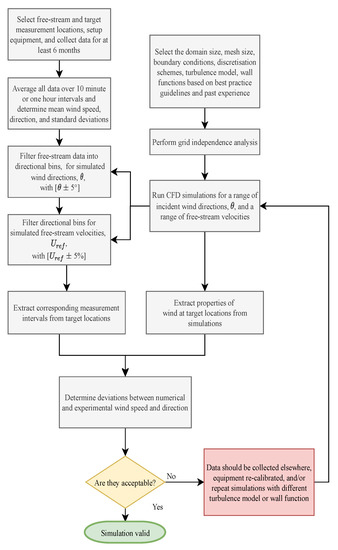
Figure 1.
Proposed urban CFD validation methodology.
In the first step of the proposed framework, measurement locations should be chosen to accurately represent the CFD model. Free, unobstructed locations should be selected to ensure the most accurate data collection. Depending on the intended use of the CFD model, the locations should be chosen in areas of great interest, i.e., a proposed turbine location, pedestrian walkways, near air intakes/exhausts, etc. Measurement equipment should be set up and data should be collected for at least 6 months. Considering the type of analysis that is intended, the proper type of measurement instrument should be chosen. If an in-depth wind resource assessment is to be conducted, including turbulence measurements, an ultrasonic anemometer should be chosen to allow for fine temporal resolution, or better, otherwise, a vane or cup anemometer with a lower temporal resolution, around or better, will be sufficient.
When all computational parameters, such as the geometry complexity and size, the choice of the turbulence model, type of wall functions, and boundary conditions are chosen, an initial simulation should be performed, and a grid independence analysis conducted. The grid should be systematically coarsened or refined, and simulations on these new grids are performed. The results of each simulation are compared until there are no significant changes and grid independence has been reached. The most efficient grid is the coarsest one that still provides grid independent results. When grid independence has been reached, the simulations should be run for a range of different incident wind directions, , and a range of free stream velocities, .
When enough data have been collected, they should be averaged over 1-h intervals to be consistent with the hourly averaged free-stream data for the validation study. It is best that the collected data to be also averaged over 10-min intervals at this stage, so they can be used in future studies of wind flow characteristics such as turbulence intensity. The most frequently used averaging period in wind engineering is 10 min, while classical boundary layer meteorology most often uses 30 min [22]. The mean direction and speed calculated, along with their standard deviations. The averaged free stream data should then be sorted into directional bins. The directional bins should correspond to the simulated incident wind directions and should only allow measured wind directions in the range of , to ensure accurate comparisons to the CFD. Each directional bin is then filtered, and data points are sorted by wind speed, filtering for the same simulated free stream velocities, within the allowable range .
Once the free stream data have been filtered, the data from the measurement positions with the same date and time ID as the binned free stream data are filtered and placed in their corresponding bins. In other words, if in the free stream bin for North () wind at , there exists a data point for April 1st at 1 AM, the data points for this same date and time at all measurement locations should be filtered and placed into bins for the same wind conditions (North at ).
The simulated wind speed and direction at the same locations as the measurement equipment are then extracted from the CFD and the error between the simulated and measured data can be determined.
When deciding if the errors are acceptable, there are many things to take into consideration. The applications of the model, the allowable error for the given application (e.g., working threshold for equipment, tolerances, etc.), the most important parameter(s) (e.g., wind speed, direction, turbulence intensity, etc.), are all questions that the modeler must ask themselves, in order to come to a decision.
2.2. CFD Model
The work done on this model was presented previously [23]. The following section reviews the main aspects of the model creation and its features.
The commercial CFD code ANSYS CFX was used for the numerical modelling of the wind flow over the University of Alberta campus. The ANSYS CFX solver engine uses a parallel, implicitly coupled multigrid solver that is tuned for industrial CFD applications. The discretization of Navier–Stokes equations is based on a hybrid finite-element/finite volume approach, and the advection fluxes are evaluated using a high-resolution scheme which is second-order accurate and bounded [23].
All the buildings in Figure 2 are modelled precisely, considering their geometric complexities for accurately modelling the wind flow over the campus. To generate the geometry, a free and open-source platform called 3D Warehouse, available via the 3D modelling computer program SketchUp [24], was utilized for its massive open-source library of three-dimensional models.
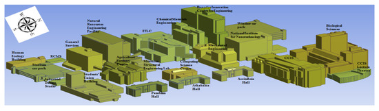
Figure 2.
CAD model of the University of Alberta designed in SolidWorks.
Some accurate models of the University of Alberta Campus obtained by photogrammetry were already available on SketchUp [24] and were thus utilized to generate fast and accurate geometries for CFD analysis. These models were imported into SolidWorks and edited, such as the trimming of excessive dimensions which have a negligible effect on the CFD analysis, such as stair rails or window details. For the other buildings not available online, architectural plans from the university were necessary for the designs.
The meshing was done using a combination of hexahedral elements to mesh simple regions, and the Delaunay meshing algorithm [25] which produced tetrahedral elements around buildings with complex shapes (Figure 3). Several prismatic layers were generated near the ground, the walls, and the roofs of buildings to capture boundary layer gradients. Smaller cells were used around small geometric details and in areas with high solution gradients (complex flow) [23].
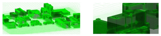
Figure 3.
Plan view of the meshed geometry. A lower resolution was used in simple regions and a high resolution in the vicinity of buildings. Inflation layers near the ground, the walls, and the roofs of buildings.
The simulated buildings were placed in a rectangular domain with a distance of (where the height of the tallest building) between the building and: the inlet, the lateral sides, and the top of the computational domain; and a distance of from the building and the outlet. It should be noted that the inlet and outlet planes are perpendicular to the free stream wind direction, and to assess every specific wind incident, the corresponding computational domain was created accordingly.
The boundary conditions at the limits of this rectangular domain were defined. The mean logarithmic velocity profile () and the turbulence quantities profiles (turbulence kinetic energy, , and its dissipation rate, ) derived from the assumption of an equilibrium boundary layer by Richards and Hoxey [26] were computed at the inlet of the computational domain [23]:
where is the friction velocity associated with the logarithmic wind speed profile, is the vertical displacement, and is the aerodynamic roughness length, is the von Karman constant, , and is a model constant, .
Over the earth’s surface, the ground experiences a ‘no slip condition’ due to the surface friction, and the velocity of the wind at the ground is effectively slowed to zero. This is the zero-plane. Theoretically, the wind speed at a height of should be zero. When flow passes over buildings, vegetation, or any other porous medium, the wind profile will be changed and shifted up, and the new zero-plane will be displaced to the top of the vegetation or other roughness elements altering the flow profile [27]. Assuming the considered terrain in this study with regular large obstacle (suburb, forest) and several buildings with various heights, the value of is an appropriate choice [28].
The value of the aerodynamic roughness length ) and a representative wind speed () at a reference height of were estimated via the Canadian Wind Atlas website, and were used to determine the friction velocity, . The shear stress transport (SST) , was chosen as the turbulence model because of its overall good performance for resolving wind flow around buildings [29]. This choice required converting the profile of to the specific dissipation rate using the relation: Therefore, the inflow profiles defined at the inlet of the computational domain were the wind speed, , the turbulence kinetic energy, , and the specific dissipation rate, .
At the outlet of the domain, zero relative pressure was imposed, while symmetry boundary conditions were applied at the top and the side faces of the computational domain to approximate the free stream flow at these boundaries far away from geometry. The roofs and the walls of all simulated buildings, as well as the ground, were set as no-slip walls and the automatic near-wall treatment method was deployed by ANSYS CFX. This allowed a gradual switch between wall functions and low Reynolds number grids to treat the wall effects within the boundary layer regions [23].
The flow characteristics in recirculation zones, near walls, and well away from it are the expected results considering the intended applications for developing this CFD model. The 3D steady RANS equations were computed in combination with the SST turbulence closure model as it is best suited to capture the turbulent flow in the areas of interest. Steady simulations were run as they are less computationally expensive and require less time per simulation, compared to unsteady simulations. High resolution schemes are used for the advection and viscous terms, and turbulence parameters of the governing equations. The normalized residual target was set to , as recommended by Franke et al. [30]. Three points upwind, one downwind of the domain, and one above the Donadeo ICE building (Edmonton, AB, Canada) roof were monitored during each simulation. The convergence was reached as the normalized residuals of the momentum and the velocity profiles, which were obtained in three locations of the domain, showed no considerable fluctuations over the iterative process [23].
A grid independence analysis was performed for ensuring that the simulated results were independent of the grid resolution. Three different grid sizes of 5,530,761 nodes (Mesh 1), 8,309,837 nodes (Mesh 2), and 11,020,616 nodes (Mesh 3) were analysed, and the results are shown in Figure 4. The wind direction was from the South and the normalized velocity profiles were taken along a vertical line above the roof, near the west edge of the Donadeo ICE building. As there were no significant differences in the profiles of the normalized velocity along the vertical direction for the three grids, the intermediate grid (Mesh 2) was chosen as the optimum grid for the simulations over the campus [23].
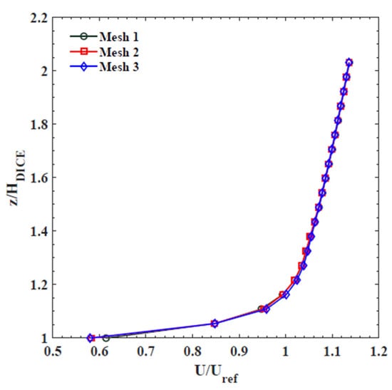
Figure 4.
Normalized velocity profiles taken along a vertical line above the Donadeo ICE roof. Taken with permission from Fogaing et al. [23].
2.3. Location and Equipment
Three anemometers were used to collect wind data: two R. M. Young Model 81000 3D ultrasonic anemometers (Figure 5a), ‘B’ and ‘D’, and one R. M. Young Model 09101 wind monitors (Figure 5b), ‘A’. The anemometers were set up around the roof of the target Donadeo ICE (Figure 6), which is located in the University of Alberta North Campus and its dimensions are tall, long and wide. Donadeo ICE is the tallest building in North Campus and has been chosen as the target building because of its height and suitable location.
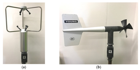
Figure 5.
(a) Young Model 81000 3D ultrasonic anemometer, (b) Young Model 09101 wind monitors.
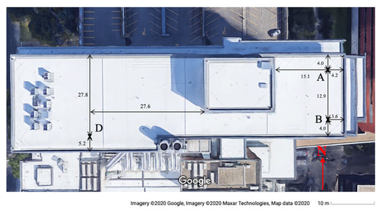
Figure 6.
Locations of anemometers on the roof of the Donadeo ICE building. Note that dimensions are in m.
Ultrasonic anemometers measure the time it takes a signal of ultrasonic frequency to travel between two transducers. To calculate the wind velocity, a sonic beam with a known frequency will be transmitted toward the receiver, which then is affected in its path by wind flow. This interaction changes the original doppler shift frequency and as a result a different frequency will be recorded by receiver. The frequency difference between source and receiver is measured by electronic circuits, and then will be used to calculate the wind velocity components. The travel time of the signal depends on both the speeds of sound and wind between two transducers that are positioned at a known distance from each other [31,32]. The ultrasonic anemometers are quite reliable and except in rare cases of harsh atmospheric conditions (heavy rain or ice buildup), they provide precise measurements [33].
Mechanical wind monitors measure two-dimensional wind speed and direction. In the 09101 monitor, the wind speed sensor is a four-blade propeller that turns a multipole magnet. The rotation induces a variable frequency signal in a stationary coil. The raw transducer signals are processed by onboard electronics; however, a conventional calibrated voltage output can be selected and processed by an external board [34]. The specifications of both pieces of equipment are presented in Table 1 below.

Table 1.
Anemometer specifications.
From Figure 6, it can be seen that there are several stacks of solar panels on the west side of the roof. It was recommended that no equipment is to be installed within of the solar panels to ensure the safety of any personnel working on the roof either around or with the solar panels.
The locations were chosen to allow us to get a more complete view of the wind flow around the building. Because of the presence and location of the elevator penthouse, regardless of the prevailing wind direction, the flow is disturbed downstream of it, and having only upstream measurements will not be an accurate representation of the entire flow field. So, it was important to have at least one anemometer that was undisturbed for all wind directions, which led to siting the anemometers as such.
Data collection was done using the National Instruments (Austin, TX, USA) software, LabVIEW. Two virtual instruments were created, one for the mechanical monitors and one for the ultrasonic anemometers. Both the mechanical and ultrasonic anemometers were set to serial outputs, RS-485 and RS-232, respectively. Serial to USB converters were employed, allowing the anemometers to connect directly to a computer. The computer, power supply, and the anemometer connections were housed in a Campbell Scientific weather resistant enclosure, ENC 16/18, that remained on the roof. To avoid damaging the computer during the harsh winter weather and rainy summers, a network connection was set up on the roof to allow for remote access to this computer, so that the enclosure is not opened when there is a need to retrieve data from the computer or any computer maintenance is required. The mechanical monitors were set to collect data at a rate of 1 Hz and the ultrasonic at a rate of 15 Hz. The recorded data were saved to a daily .txt file, with a naming convention of “month, day, year”.
2.4. Data Processing
The equipment was set up on 30th November 2018, and the continuous data collection began on 8th February 2019. While the data collection remains ongoing, for the scope of this paper, the data processed and analyzed were limited to the six months of 8th February to 8th August 2019. Note that there are a few days of data that were not collected throughout the dataset, due to power interruptions and scheduled maintenance of the engineering network.
For a reference wind speed and direction, data from the University of Alberta, Earth and Atmospheric Science (EAS) Department weather station on the roof of the University of Alberta’s Henry Marshall Tory Building were used. This building is the tallest within its immediate vicinity, at 57 m tall, with all the surrounding buildings significantly lower. The weather station is positioned at 64 above the ground (7 m above the top of the building) and appears to be sufficiently elevated above the surrounding ground and building roughness elements. This building is positioned in University of Alberta North campus and is located approximately 1 km east of Donadeo ICE building (the target location). Because of this, we chose to consider the measurements as a “free stream” reference point for wind analysis on campus. The weather station consists of a RM Young 05103 mechanical monitor and a Campbell Scientific CR10X data logger. The data are measured at a rate of roughly and are averaged and archived as hourly wind data. The archives date back to July 2000, meaning we could use reference measurements for the same six months period of 8th February to 8th August 2019, for our analysis. The Tory weather station (TWS) provides hourly averaged data for solar radiation, rain, temperature, relative humidity, and barometric pressure, along with 2D wind speed and wind direction.
3. Results and Discussion
Following the validation methodology that was created and presented in Section 2.1, wind flow around the campus was simulated and analyzed for four inflow wind directions, (North), (East), (South), and (West). Based on the Canadian Wind Atlas website, the reference wind speed at University of Alberta North campus, , at a height of was dominantly varied between . Therefore, this range was considered to filter the collected measurements for validation study.
Data were collected for six months and as previously discussed, the TWS only provides hourly averages for the free stream data, so the Donadeo ICE data were averaged into hourly intervals. The TWS data were then filtered for the same inflow direction and speeds as was simulated and 36 bins were created for the free stream flow. The number of resultant data points (hourly averages) in each bin can be found in Table 2.
Table 2.
Number of measurement samples (hourly averaged) for each free stream bin.
As can be seen, there are several bins for which no measurements fit the criteria, so only free stream velocities of and were considered for the validation process. The Donadeo ICE data at positions A, B, and D were then filtered and the measurement intervals corresponding to those in the free stream bins were obtained and placed into bins of their own. It is important to note here that only a limited number of measurements were selected as validation points because of the strictness of the acceptance criteria, namely, the allowable range allotted to a given bin. This allows us to test the validity of the model under very precise conditions, which can ensure that any issues with the model can be exposed. Because of the short duration of this project, a test of validity with more lenient criteria and a comparison between the two could not be done but was suggested for future work.
To calculate the difference between the experimental and numerical results, two methods were used. The first method (from here on, “the average method,” AM) took all measurements in the bins and an average value of wind speed and direction were calculated, and then used to compare to the CFD results, as it is commonly done in literature [11,12,13,35,36]. The second proposed method (from here on, “the standard deviation method,” SDM) consisted of comparing the measurement which had the least variability in the wind direction with the CFD results. The date and time of the TWS measurement that had the lowest wind direction standard deviation in each bin were noted, and the corresponding Donadeo ICE measurement was used to compare with CFD. Both these methods were used to ensure that the best validation technique was being applied, and to assess any differences that arise from the application of different validation methods.
Radial plots were used to show the differences between the numerical and experimental results for a given wind speed and direction at each measurement location, and the scatter plots were used to assess the overall correlation of the simulated and measured results at all locations and all incident wind directions. The scatter plots are shown in Figure 7 and Figure 8 below. Note that SDM and AM correspond to the standard deviation method and average method, respectively. The solid line represents a perfect agreement between the simulated and measured results, and the dashed lines represent a 10% deviation. A, B, and D are the three anemometer measurement locations.
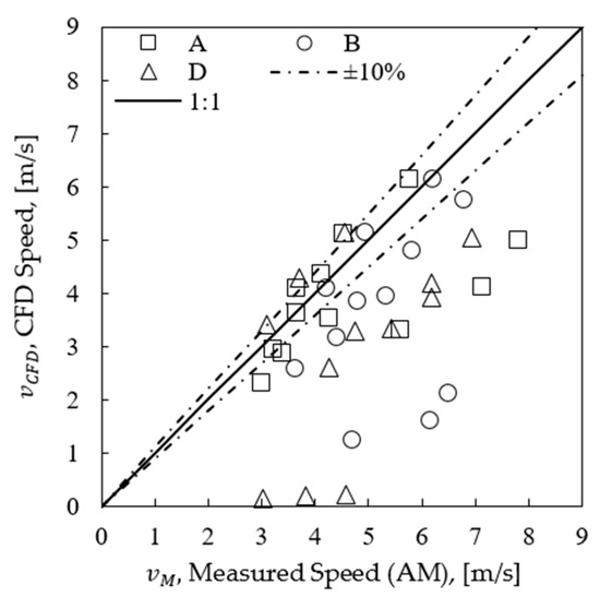
Figure 7.
Comparison between the measured and simulated speeds at measuring locations (A, B, and D), using the average method.
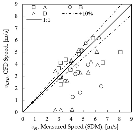
Figure 8.
Comparison between the measured and simulated speeds at measuring locations (A, B, and D), using the standard deviation method.
As previously indicated, the objective of these plots is not to assess the exact deviations of the model from the measured speeds, but to see the overall agreement of the CFD results with the measured results, using the different comparison methods. The first clear inference we can make from these plots is that the CFD is more consistently underestimating the speed, regardless of the method of analysis used.
Comparing Figure 7 with Figure 8, we can see that there are very minor differences between the standard deviation method and the average method. However, the numerical results seem to be a slightly better representation of the measured results when the standard deviation method of analysis is used. The results for the standard deviation method appear to shift closer to and have an overall closer fit to the 1:1 ratio line. This is not unexpected, as the standard deviation method used the hours which had the least wind variability, meaning the wind direction was more consistently blowing in the same direction, which is better reproduced by a CFD simulation.
The radial comparisons at all locations (A, B, D) for a free stream velocity of are shown in Figure 9 and Figure 10 below.
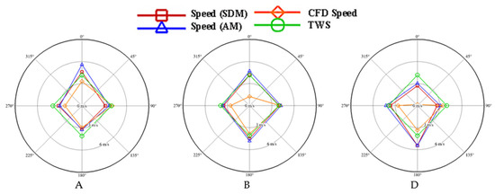
Figure 9.
Comparison of measured and simulated wind speeds at all locations (A,B,D).
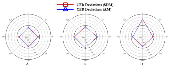
Figure 10.
Deviation of simulated wind direction from measured wind direction at all locations (A,B,D).
Figure 9 contrasts the differences between the measured and simulated wind speeds for all incident wind directions, and Figure 10 presents the deviations of the simulated wind direction to the measured wind direction for all incident winds. The solid black line represents a deviation (i.e., exact match), represents a clockwise deviation, and represents a counterclockwise deviation of the numerical results from the experimental results.
Examining Figure 9 confirms the initial inferences made, as we can see that the numerical results seem to be a better representation of the measured speeds when the standard deviation method of analysis is used, and we can observe that for all locations, the CFD is almost always underestimating the speed, as previously deduced by the scatter plots. From these radial plots, we can also see that at all locations, the largest deviations between the simulated and measured speeds are consistently for winds from the North, followed by West and South, in that order. The simulated speeds for East winds seem to have regularly good agreements with the experimental values, for both methods of analysis used, at all locations.
When examining Figure 10, however, there only seem to be slight and insignificant differences between the standard deviation and average methods for the wind direction at most for most locations and incident wind directions. The plots show that at locations (A, B), there is a good agreement between the measured and simulated wind directions, with most deviations less than , and a few less than . This is comparable to the results found by Blocken et al. [12], who had average deviations of and for all directions at both measurement locations.
From Figure 10, we find that the numerical estimates of the North wind produce a seemingly isolated large deviation from the measured at that location, for both the speed and direction. Upon further inspection of the simulations for the North wind, it is evident that the measurement location (D) falls within a recirculation zone, as shown in Figure 11, which is the cause of this inconsistency.
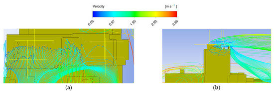
Figure 11.
Recirculation over Donadeo ICE for North winds at 4 m/s (a) top view (b) side view.
The average absolute deviations between the CFD results and the measured results were tabulated to better quantify the validity of the simulations. Since Anemometer D was situated in a recirculation zone, for incident winds coming from the North, this measurement was taken out of the study and will not be considered when making a final assessment. The values in Table 3 were calculated by taking the absolute value of the difference between the numerical results and the experimental results at all locations for each incident wind direction and free stream speed and finding the average. The decision to consider all locations for any given incident wind direction was made as there was no clear distinction or distinguishing pattern between the deviations from the upstream and downstream measurement points for us to consider.
Table 3.
Average deviations in speed and direction for each incident wind direction.
The deviation in speed for the standard deviation method ( for North winds at was calculated as follows:
The italics in Table 3 denote the smallest deviation (closest agreement between the measured and numerical results) between the standard deviation method and the average method. We can see that the standard deviation method produced smaller deviations more frequently, as 16 of the 24 numerical deviations were better agreements with the measured values, most commonly for deviations in speed. Table 4 presents the corresponding average percent error of the deviations between numerical and experimental speeds for each incident wind direction.
Table 4.
Average percent error of numerical speeds for each incident wind direction.
As previously mentioned, the largest deviations for speed are consistently for winds from the North, which is confirmed by the results in Table 3 and Table 4. We can also see that at , the deviations in the wind direction are largest for the winds from the West and South. Looking at the simulated geometry in Figure 12, we can immediately note that the Donadeo ICE building and the attached car park are at the Northwest edge, and the surroundings to the North and West of the building are not modelled, which could be the cause of the large deviations. The deviations for South winds could be attributed to some simplifications to the geometrical details of the surrounding buildings. In addition, the North Saskatchewan River runs in a deep valley around the University of Alberta and is immediately North and West of the Donadeo ICE building, separated by some homes, parks, and vegetation.
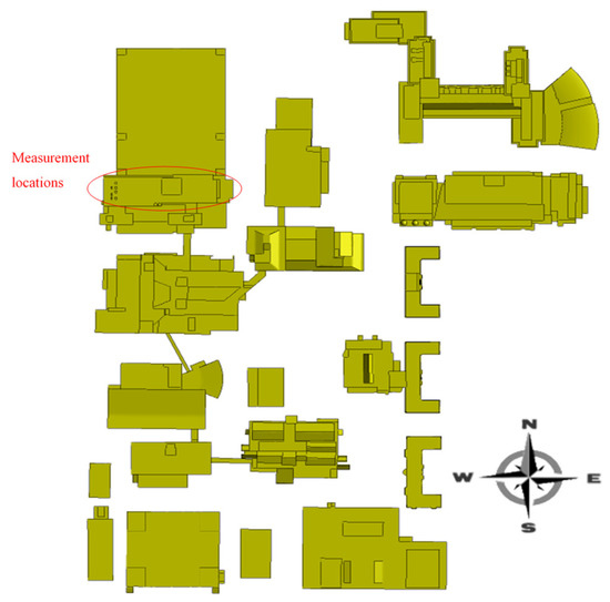
Figure 12.
CFD geometry.
During the day, the surface of the land warms up at a higher rate compared to water due to its relatively lower thermal capacity. Consequently, the warmer air adjacent to land starts to rise up and the resultant pressure difference drives the local wind above the water toward the land. The opposite happens at nights, as the land surface cools down much faster than the water and local winds will be forced toward the water [37]. This phenomenon creates a wind flow stream towards the measurement location on Donadeo ICE building, which is not considered in the presented CFD model.
Based on the presented data and the calculated deviations between the numerical and experimental results, the proposed methodology and CFD simulations are deemed valid for the East and South directions. However, this claim cannot be made for wind incidents coming from North and West. As it was fully described before, the inaccurate modeling of the upstream geometry is the main reason for calculating relatively higher deviations in these two cases.
Considering that the presented SDM approach in this paper uses the selected data of occasions with relatively constant wind characteristics and small variability, it is more appropriate to be used for validating the reproduced flow field by CFD. Additionally, as this approach utilizes the square of the deviations in its calculations, it amplifies the contribution of deviations that are larger comparatively and a much more strict and reliable error analysis will be possible as the result. However, careful considerations are definitely required in choosing the measurement locations. Calculating the associated error using this approach, will lead to excessive overestimation of the overall deviation in recirculation zones.
It is suggested that data should be collected for at least one year and a complete wind resource assessment should be conducted prior to running any simulations. The predominant and most frequent wind directions and speeds should be determined, and the simulations should be run accordingly. Allowable range for measurement bins could also be increased to have more data available to be implemented in error analysis methods presented.
4. Conclusions
The goal of this paper was to conduct an experimental measurement campaign to provide data for the creation of a framework for the validation of a CFD model assessing the rooftop wind regime around buildings of the University of Alberta North Campus. This CFD model can be used for wind turbine location sitting for urban wind power generation, improving the efficiency of HVAC systems, building and urban planning, and improving the design of building exhaust stacks for better dispersion.
To collect data, an experimental measurement campaign was first designed and installed on the roof of the Donadeo ICE building, which was the target of the CFD study. Three anemometers, two ultrasonic and one mechanical wind monitor, measuring at 15 Hz and 1 Hz, respectively, were set up around the building in a way that would allow us to get a more complete view of the wind flow around the building, so they were set up around the three corners of the roof, within a safe working distance of the West edge, due to the presence of some stacked solar panels. The anemometers were installed on 15 ft masts. A data acquisition system was designed using the software LabVIEW. Measurements from the TWS on campus were used as reference free stream data. Data were collected for six months and were processed and analyzed using the statistical software RStudio. The data were averaged into one-hour increments, to allow us to accurately compare with the TWS data, as it is hourly averaged and archived.
Simulations were run for a range of wind speeds and directions, and the experimental data were filtered and placed into directional bins, and two methods were also used to compare with the numerical results. The first method was the standard deviation method, which used the measurement with the calmest winds (smallest standard deviation of the wind direction for the hourly average) to compare with the numerical results. The second method was the average method, which took the average of all measurements in each bin and compared to the numerical results. The key results are:
- The standard deviation method was found to produce slightly better agreements between the numerical and experimental results more frequently than the average method.
- 16 of the 24 numerical deviations were better agreements with the measured values using the standard deviation method, most commonly for deviations in speed.
- Average wind speed errors of 10.8% and 17.7% were calculated for cases of East and South wind incidents, respectively. The corresponding wind direction deviation for these incidents were also calculated as and , respectively. Considering the calculated errors, the presented CFD model is valid for East and South wind directions.
- The calculated errors between the measured and simulated speeds for North and West wind directions are higher with values of 51.2% and 24.6%, respectively. Deviations of and in wind directions were also calculated for the mentioned wind incidents in the same order. The main reason for calculating these relatively higher deviations and errors is the fact that upstream geometry was not modeled in detail for the West and North directions.
- Considering the good agreement that were reached between the numerical and experimental results for the East and South directions, the presented validation methodology in this work is acceptable.
Author Contributions
Conceptualization, S.J.M. and B.A.F.; methodology, S.J.M., B.A.F. and C.F.L.; software, S.J.M.; validation, S.J.M.; formal analysis, S.J.M.; investigation, S.J.M.; resources, B.A.F.; data curation, S.J.M.; writing—original draft preparation, S.J.M., M.R.K.N.; writing—review and editing, S.J.M., M.R.K.N., B.A.F., C.F.L.; visualization, S.J.M.; supervision, B.A.F. and C.F.L.; project administration, B.A.F. and M.V.; logistic planning and site supervision, B.A.F. and M.V.; funding acquisition, B.A.F. All authors have read and agreed to the published version of the manuscript.
Funding
This research was funded by Energy Management and Sustainable Operations (EMSO).
Institutional Review Board Statement
Not applicable.
Informed Consent Statement
Not applicable.
Data Availability Statement
Data supporting the reported result can be found here [38].
Acknowledgments
The authors would like to thank M.B. Tadie Fogaing for providing the CFD model and grid.
Conflicts of Interest
The authors declare no conflict of interest.
References
- UNFCCC. Adoption of the Paris Agreement. In Proceedings of the Conference of the Parties COP 21, Paris, France, 30 November–11 December 2015. [Google Scholar]
- Hydro-Quebec. Ontario Rebate for Electricity Consumers Act, 2016; Westario Power: Toronto, ON, Canada, 2019; Volume 22, pp. 1–11. [Google Scholar]
- Hydro-Quebec. Net Metering Rate Option for Self-Generators; Hydro-Quebec: Montreal, QC, Canada, 2019. [Google Scholar]
- BC Hydro. Our Distributed Generation Programs; BC Hydro: Vancouver, BC, Canada, 2019. [Google Scholar]
- Alberta Queen’s Printer. Electric Utilities Act. Micro-Generation Regulation; Alberta Queen’s Printer: Edmonton, AB, Canada, 2018.
- Alberta Electric System Operator. Micro-Generation in Alberta; Alberta Queen’s Printer: Edmonton, AB, Canada, 2018.
- Versteege, M.; Leblanc, S. Energy Reduction Master Plan 2017–2020. University of Alberta Facilities and Operations: Edmonton, AB, Canada, 2017. [Google Scholar]
- Blocken, B. 50 years of computational wind engineering: Past, present and future. J. Wind Eng. Ind. Aerodyn. 2014, 129, 69–102. [Google Scholar] [CrossRef]
- Simões, T.; Estanqueiro, A. A new methodology for urban wind resource assessment. Renew. Energy 2016, 89, 598–605. [Google Scholar] [CrossRef]
- Fogaing, M.B.T.; Gordon, H.; Lange, C.F.; Wood, D.H.; Fleck, B.A. A review of wind energy resource assessment in the urban environment. In Advances in Sustainable Energy; Vasel, A., Ting, D.S.-K., Eds.; Springer International Publishing: Cham, Switzerland, 2019; pp. 7–36. [Google Scholar]
- Blocken, B.; Persoon, J. Pedestrian wind comfort around a large football stadium in an urban environment: CFD simulation, validation and application of the new Dutch wind nuisance standard. J. Wind Eng. Ind. Aerodyn. 2009, 97, 255–270. [Google Scholar] [CrossRef]
- Blocken, B.; Janssen, W.D.; van Hooff, T. CFD simulation for pedestrian wind comfort and wind safety in urban areas: General decision framework and case study for the Eindhoven University campus. Environ. Model. Softw. 2012, 30, 15–34. [Google Scholar] [CrossRef]
- Kalmikov, A.; Dupont, G.; Dykes, K.; Chan, C. Wind Power Resource Assessment in Complex Urban Environments: MIT Campus Case-Study Using CFD Analysis. In Proceedings of the AWEA 2010 Wind Conference, Dallas, TX, USA, 7–9 December 2010; p. 2010. [Google Scholar]
- Tabrizi, A.B.; Whale, J.; Lyons, T.; Urmee, T. Performance and safety of rooftop wind turbines: Use of CFD to gain insight into inflow conditions. Renew. Energy 2014, 67, 242–251. [Google Scholar] [CrossRef]
- Tabrizi, A.B.; Whale, J.; Lyons, T.; Urmee, T. Rooftop wind monitoring campaigns for small wind turbine applications: Effect of sampling rate and averaging period. Renew. Energy 2015, 77, 320–330. [Google Scholar] [CrossRef]
- Wang, Q.; Wang, J.; Hou, Y.; Yuan, R.; Luo, K.; Fan, J. Micrositing of roof mounting wind turbine in urban environment: CFD simulations and lidar measurements. Renew. Energy 2018, 115, 1118–1133. [Google Scholar] [CrossRef]
- Liu, S.; Pan, W.; Zhang, H.; Cheng, X.; Long, Z.; Chen, Q. CFD simulations of wind distribution in an urban community with a full-scale geometrical model. Build. Environ. 2017, 117, 11–23. [Google Scholar] [CrossRef]
- Liu, S.; Pan, W.; Zhao, X.; Zhang, H.; Cheng, X.; Long, Z.; Chen, Q. Influence of surrounding buildings on wind flow around a building predicted by CFD simulations. Build. Environ. 2018, 140, 1–10. [Google Scholar] [CrossRef]
- Tang, X.Y.; Zhao, S.; Fan, B.; Peinke, J.; Stoevesandt, B. Micro-scale wind resource assessment in complex terrain based on CFD coupled measurement from multiple masts. Appl. Energy 2019, 238, 806–815. [Google Scholar] [CrossRef]
- Toparlar, Y.; Blocken, B.; Vos, P.; van Heijst, G.J.F.; Janssen, W.D.; van Hooff, T.; Montazeri, H.; Timmermans, H.J.P. CFD simulation and validation of urban microclimate: A case study for Bergpolder Zuid, Rotterdam. Build. Environ. 2015, 83, 79–90. [Google Scholar] [CrossRef]
- Franke, J.; Sturm, M.; Kalmbach, C. Validation of OpenFOAM 1.6.x with the German VDI guideline for obstacle resolving micro-scale models. J. Wind Eng. Ind. Aerodyn. 2012, 104–106, 350–359. [Google Scholar] [CrossRef]
- Emeis, S. Wind Energy Meteorology Atmospheric Physics for Wind Power Generation, 2nd ed.; Springer: Cham, Switzerland, 2018. [Google Scholar]
- Fogaing, M.B.T.; Yalchin, J.; Shadpey, S.; Lange, C.F.; Fleck, B.A. Numerical assessment of rooftop wind regime around buildings in a complex urban environment. In Proceedings of the 26th Annual Conference of the CFD Society of Canada, Winnipeg, MB, Canada, 10–12 June 2018. [Google Scholar]
- 3D Warehouse. 2018. Available online: https://3dwarehouse.sketchup.com/ (accessed on 11 February 2018).
- ANSYS Inc. Quick (Delaunay); ANSYS: Canonsburg, PA, USA, 2019. [Google Scholar]
- Richards, P.J.; Hoxey, R.P. Appropriate boundary conditions for computational wind engineering models using the k-ε{lunate} turbulence model. J. Wind Eng. Ind. Aerodyn. 1993, 46–47, 145–153. [Google Scholar] [CrossRef]
- Landberg, L. Meteorology for Wind Energy; Springer: Cham, Switzerland, 2016. [Google Scholar]
- WMO Guide to Meteorological Instruments and Methods of Observation; WMO-No. 8; WMO: Geneva, Switzerland, 2006; pp. I.5–I.13.
- Mohamed, M.A.; Wood, D.H. Computational modeling of wind flow over the University of Calgary campus. Wind Eng. 2016, 40, 228–249. [Google Scholar] [CrossRef]
- Franke, J.; Hellsten, A.; Schlünzen, H.; Carissimo, B. Guideline for the CFD Simulation of Flows in the Urban Environment: COST Action 732 Quality Assurance and Improvement of Microscale Meteorological; Meteorological Institute: Geneva, Switzerland, 2007.
- Kelton, G.; Bricout, P. Wind velocity measurements using sonic techniques. Bull. Am. Meteorol. Soc. 1964, 45, 571–580. [Google Scholar] [CrossRef][Green Version]
- Woodford, C. Anemometers. 2009. Available online: https://www.explainthatstuff.com/anemometers.html (accessed on 27 July 2019).
- Center for Atmospheric Science, Sonic Anemometers. Available online: http://www.cas.manchester.ac.uk/restools/instruments/meteorology/sonic/ (accessed on 27 July 2019).
- Wind Monitor-SE Model 09101 instruction manual; R. M. Young Company: Traverse City, MI, USA, 2017.
- Blocken, B.; van der Hout, A.; Dekker, J.; Weiler, O. CFD simulation of wind flow over natural complex terrain: Case study with validation by field measurements for Ria de Ferrol, Galicia, Spain. J. Wind Eng. Ind. Aerodyn. 2015, 147, 43–57. [Google Scholar] [CrossRef]
- Dhunny, A.Z.; Lollchund, M.R.; Rughooputh, S.D.D.V. Wind energy evaluation for a highly complex terrain using Computational Fluid Dynamics (CFD). Renew. Energy 2017, 101, 1–9. [Google Scholar] [CrossRef]
- Chen, Q. Using computational tools to factor wind into architectural environment design. Energy Build. 2004, 36, 1197–1209. [Google Scholar] [CrossRef]
- Mattar, S.J. Computational Fluid Dynamics Validation of Rooftop Wind Regime in Complex Urban Environment. Master’s Thesis, University of Alberta, Edmonton, AB, Canada, 2019. Available online: https://era.library.ualberta.ca/items/5f6a8cf1-3960-4aa9-9641-ea9390285c05/view/888c2107-9ac8-403a-828e-3221ca93bcae/Mattar_Sarah_201912_MSc.pdf (accessed on 27 July 2019).
Publisher’s Note: MDPI stays neutral with regard to jurisdictional claims in published maps and institutional affiliations. |
© 2021 by the authors. Licensee MDPI, Basel, Switzerland. This article is an open access article distributed under the terms and conditions of the Creative Commons Attribution (CC BY) license (https://creativecommons.org/licenses/by/4.0/).