Article

Robust Inverse Optimal Control for a Boost Converter

by
Mario Villegas-Ruvalcaba
1,
Kelly Joel Gurubel-Tun
2 and
Alberto Coronado-Mendoza
2,*
1
Basic and Applied Sciences Department, University of Guadalajara, Guadalajara 45425, Mexico
2
Studies on Water and Energy Department, University of Guadalajara, Guadalajara 45425, Mexico
*
Author to whom correspondence should be addressed.
Energies 2021, 14(9), 2507; https://doi.org/10.3390/en14092507
Submission received: 15 March 2021 / Revised: 14 April 2021 / Accepted: 22 April 2021 / Published: 27 April 2021
(This article belongs to the Section F: Electrical Engineering)

Abstract

:
The variability of renewable energies and their integration into the grid via power electronics demands the design of robust control algorithms. This work incorporates two techniques to ensure the stability of a boost converter through its state equations, implementing the inverse optimal control and the gain-scheduling technique for robust control settings. In such a way that, under a single adjustment, it is capable of damping different changes such as changes in the parameters, changes in the load, the input voltage, and the reference voltage. On the other hand, inverse optimal control is based on a discrete-time control Lyapunov function (CLF), and CLF candidate depends on fixed parameters that are selected to obtain the solution for inverse optimal control. Once these parameters have been found through heuristic or artificial intelligence methods, the new proposed methodology is capable of obtaining a robust optimal control scheme, without having to search for new parameters through other methods, since these are sometimes sensitive changes and many times the process of a new search is delayed. The results of the approach are simulated using Matlab, obtaining good performance of the proposed control under different operation conditions. Such simulations yielded errors of less than 1% based on the voltage reference, given the disturbances caused by changes in the input variables, system parameters, and changes in the reference. Thus, applying the new methodology, the stability of our system was preserved in all cases.

1. Introduction

Power converters have been a fundamental piece for the integration of renewable energies, which every day have a greater presence around the world [1,2,3]. The boost converter is widely used to ensure the operation of electrical systems, such as photovoltaic systems [4,5], microgrids [6,7], and fuel cells [8,9,10,11]. For this, there are different topologies according to the needs of low or high power systems [5,12]. To ensure the desired output of the boost converter, control techniques of a pulse width modulated signal (PWM) are used. Different control techniques have been used to control the desired signals for the boost converter and other converters, such as the PI [8,13,14,15,16], PID [17,18,19], frequency-domain control techniques such as the method of sliding modes [6,20,21], fuzzy logic [22,23], and inverse optimal control [24,25,26].
The equations of state of power converters are sensitive to different disturbances, which is why many works focus on damping the effects of these separately with the methods mentioned above. To mention some of them, in [17] they subject a boost converter to changes in the input variables and changes in the reference voltage separately, in [6] the disturbance is a change in the voltage reference, with fixed parameters, in [20] they subject a boost converter to variations in the load and changes in the sampling time of the control method, in [14] they subject it to changes in the voltage reference, as well as in [27], where they model different power conditioners under different initial conditions and different reference voltages, obtaining good results, using an adjustment similar to this work, however, the reference voltage changes are analyzed separately, not the subject to so many changes, nor is the extent of the adjustment analyzed. In [28], through Lyapunov’s control theory, they subject the boost converter to disturbances in the load and input voltage. In [25,26], the inverse optimal control is implemented to a boost converter, while in [26] it does not have any disturbance, and in [25] the system is tested against a voltage drop of 3 volts.
The main problem is that solving the optimal control of nonlinear systems is extremely difficult because it must be solved by Hamilton-Jacobi-Bellman (HJB) equation, and its solution may not exist [29]. The inverse optimal control approach of discrete-time nonlinear systems avoids the need to solve the associate HJB equation through the Control Lyapunov Function (CLF) [25,30,31], and this is because the CLF is a solution to a family of HJB equations [30,32]. Besides, the existence of CLF implies the stability of the system [31]. The CLF candidate depends on fixed parameters that are selected to obtain the solution for inverse optimal control. Such parameters can be difficult to find since they depend on the specific characteristics and conditions of the system. Heuristic methods have been used to find these parameters, like in [24,25] or [26,33,34,35], PSO was used, while GA was used in [32].
On the other hand, the adaptive control method by gain scheduling has been implemented to stabilize continuous non-linear systems through state space [27,36,37,38]. Furthermore, it has been used for the adjustment of different control techniques, such as sliding modes [27], Lyapunov’s control theory [37,38], even for the elaboration of mixed control schemes [39,40].
The main contribution of this work is to provide a methodology which shows a way to integrate the inverse optimal control technique and the gain scheduling technique. To do it, an analysis of the scope of the inverse optimal control is made using gain scheduling to adjust the output voltage of a boost converter. This analysis includes quantitative data that allows us to compare the adjustment provided. As a result of the implementation of said methodology, a single control adjustment coefficient is defined, which is capable of damping the effects of the perturbations of the parameters of the boost converter state equations, as well as changes in the input variables, changes in output voltage, and changes in sequence in reference signals. In addition to providing a methodology that facilitates the search for the necessary parameters for the implementation of the inverse optimal control under certain conditions, this methodology also serves for changes in the sampling time.
This paper has the next structure. Section 2 describes the boost converter structure and its state equations. In Section 3, the inverse optimal control model is presented. In Section 4, the methodology of the changes in the control law is described. In Section 5, the inverse optimal control is applied to the boost converter to show some control problems. In Section 6, the results of the new methodology applied to the boost converter are discussed. Finally, the conclusions are in Section 7.

2. State Equations Model of the Boost Converter

The classic diagram of the boost converter is shown in Figure 1, which is composed of a diode, a switch (IGBT), an inductance, a capacitance, and a resistance. Of which, through Kirchhoff’s laws for voltage and current, its equations can be defined [20,21,24,27,28].
Such equations are defined by the state variables, which in our case are the inductor current and the capacitor voltage. The dynamics of the system variables are described by:
d i L d t = 1 L v 1 v 0 U
d v 0 d t = 1 C i L U v 0 R L
Where v 0 is the capacitor voltage, i L is the inductor current, v 1 is the input voltage (from the source), L is the inductance of the inductor, C is the capacitance of the capacitor, R L a resistance, and U is the signal control, whose values can be 0 or 1 . Such value of U describes the states of the switch ( U = 0 open, U = 1 closed), and the process to arrive at Equations (1) and (2) is described in [24].

3. Trajectory Tracking Inverse Optimal control

Let us consider the discrete-time affine nonlinear system given in Equation (3):
x k + 1 = f x k + g x k u k ,       x 0 = x 0
Where x k n is the state of the system at time k + 0 = 0 ,   1 ,   2 ,   ,   u k m is the input, f :   n n and g : n n × m are smooth mappings, f 0 = 0 and g x k 0 for all x k 0 .
With the following cost functional associated with trajectory tracking:
J z k = n = k l z n + u n T R u n
Where z k = x k x δ , k with x δ , k as the desired trajectory for x k ; z k n ;   J z k   : n + ;   l z k   :   n + is a positive semidefinite function, and R : n n × m is a real symmetric positive definite weighting matrix. Additionally, a performance measure is the cost functional expressed by Equation (4) [26]. The entries R can be fixed or functions of the system state to vary the weighting on control efforts according to the state value [26]. Considering the state feedback control design problem, the complete state x k is assumed to be available.
Using the optimal value function J * z k for Equation (4) as Lyapunov function V x k , Equation (4) can be rewritten as
V z k = l z k + u k T R u k + n = k + 1 l z n + u n T R u n
V z k = l z k + u k T R u k + V z k + 1  
where we require the boundary condition V 0 = 0 so that V z k becomes a Lyapunov function.
The optimal control law must satisfy the next conditions. We define the discrete-time Hamiltonian H z k ,   u k as
H z k ,   u k = l z k + u k T R u k + V z k + 1   V z k
A necessary condition that the optimal control law should satisfy is
δ H z k ,   u k δ u k = 0
then
0 = 2 R u k + δ V z k + 1 δ u k 0 = 2 R u k + δ z k + 1 δ u k δ V z k + 1 δ z k + 1
0 = 2 R u k + g T x k δ V z k + 1 δ z k + 1
therefore, the optimal control law to achieve trajectory tracking is formulated as
u k * = 1 2 R 1 g T x k δ V z k + 1 δ z k + 1
with the boundary condition V 0 = 0 . For determining the trajectory tracking inverse optima control, it is necessary to solve the following HJB equation
l z k + V z k + 1 V z k + 1 4 δ V T z k + 1 δ z k + 1 g x k R 1 g T x k δ V z k + 1 δ z k + 1 = 0
which is a challenging task. The inverse optimal control solves this task because the main characteristic of inverse optimal control is that a stabilizing feedback control law is designed first, and then it is established that this law optimizes the cost functional given in Equation (4) [26].
Definition 1.
Tracking Inverse Optimal Control Law
Consider the tracking error as z k = x k x δ , k , x δ , k being the desired trajectory for x k . Let us define the control law:
u k * = 1 2 R 1 g T x k V z k + 1 z k + 1
It is inverse optimal if:
i.
Tracking Inverse: It achieves (global) asymptotic stability of x k = 0 for system Equations (1) and (2) along with reference x δ , k ;
ii.
Second V z k is a (radially unbounded) positive definite function such that inequality
V ¯ : = V z k + 1 V z k + u k * T R x k u k * 0
is satisfied.
When we select l z k : = V ¯ , the V z x is a solution for Equation (9) and the cost functional expressed by Equation (4) is minimized.
As established in Definition (1) the inverse optimal control law for trajectory tracking is based on the knowledge of V z k . For this reason, we proposed a CLF, V z k , such that (i) and (ii) are guaranteed. In this way, instead of solving Equation (9) for V z k , a quadratic CLF candidate V z k for the Equation (10) is proposed as follows:
V z k = 1 2 z k T P z k , P = P T > 0
To ensure stability of the tracking error z k , where
z k = x k x δ , k z k = x 1 , k x 1 δ , k x 2 , k x 2 δ , k x n , k x n δ , k
moreover, it will be established that the control law expressed by Equation (10) with Equation (12), which is referred to as the inverse optimal control law, optimizes a cost functional of Equation (4) [26].
Consequently, by considering V x k as in Equation (12), control law expressed by Equation (10) takes the following form:
u k * = 1 4 R g T x k δ z k + 1 T P z k + 1 δ z k + 1 u k * = 1 2 R g T x k P z k + 1 .
u k * = 1 2 R + 1 2 g T x k P g x k 1 g T x k P f x k x δ , k + 1
Where 1 2 g T x k P g x k is positive definite and symmetric matrix, which ensures that the inverse matrix in Equation (14) exists.

4. The Proposed Methodology

A new method is proposed to be able to adjust the control once it has been previously tuned under certain values and by changing these values, such as the integration step or the control objective, the control objective is reached again.
Given the following Equation (14) modifying the coefficient 1 / 2 when the control leads to the output to stagnate in a fixed error in a steady state. Changing Equation (14) by Equation (15), as follows:
u k * = K R + 1 2 g T x k P g x k 1 g T x k P f x k x δ , k + 1
The goal is to find K that tunes the control u , as in our case, u is the duty cycle and can take values from 0 to 1, which represent 0 and 100%, respectively. The above without modifying the matrix P and the R value of the control.
The proposed methodology is as follows:
  • To find the values of P and R that cause the system to converge to a target value, there are heuristic search methods.
  • Give values to the input variables, and the parameters of the system and analyze which are the ranges of those variables that generate an error ξ greater than tolerance ε .
  • Find a K value for each desired input variable or target in the ranges or values of the previous point that fit the model to the desired reference.
  • Implement different K s found in the simulation for the different values of the input variables.
  • Fit the coefficients found to an equation that depends on the input variable or the parameter that destabilized the system.
  • In the case that an appropriate value of K is not found, which adjusts the desired model for a value of the input variable or the desired objective, once again tune the model looking for appropriate P and R .
In this work, ξ is taken as the percentage error when the system falls into a steady-state error, in other words, when the error converges to a point close to the reference. Taking a tolerance ε = 1 % error with respect to the reference. Consequently, there may be different K s fits that satisfy ξ < ε .

5. Inverse Optimal Control Applied for a Boost Converter

The relation between the output voltage and the output current can be determined from the equilibrium point of the system given by Equations (1) and (2), obtaining
x 2 , k = v r e f   ,   x 1 , k = x 2 , k 2 R L v 1
With x 2 as the output voltage, x 1 the output current, and v r e f the reference voltage. To implement the inverse optimal control, Equations (1) and (2) are taken to obtain f x k and g x k from Equation (14), as follows:
f x = x 1 , k + T v 1 / L   x 2 , k T x 2 , k / R L C
and
g x = T x 2 , k / L T x 1 , k / C
discretizing by Euler approximation, the discrete-time model for the boost converter is
x 1 , k + 1 = x 1 , k + T v 1 L x 2 , k L u k
x 2 , k + 1 = x 2 , k + T x 2 , k R L C + x 1 , k C u k
where T is sampling time, and initial conditions are x 0 = 0   0 T .
First, the inverse optimal control is implemented to appreciate the effect of the change in voltage reference. Taking the fixed parameters L = 12   m H , R L = 220   Ω , C = 500   μ F , the sampling time T = 100   μ s , and the input voltage of v 1 = 80 V with reference voltage v r e f = 100 V. To implement the optimal inverse control, it is necessary to search for P and R to stabilize the system, for this, any search method can be used. In [33], the PSO is used to achieve it, and in [24], a heuristic method is used. To find a P and R that fit our system, we take a P   and R used in [24], since the same system of equations is used, but with different parameters. To do this, an exhaustive search was made, around each element of the known matrix P and R , along an interval for each element, obtaining as a result:
P = 10.06 0 0 0.003 ,   R = 0.8
Such values are necessary in Equation (14). Figure 2a shows the implementation of the inverse optimal control with a reference voltage of v r e f = 100 V with ξ 0.65 %, in Figure 2b, a change in the reference voltage from 100   V to 120   V is applied, and the output voltage never converges to the voltage reference, whose percentage of error reaches values of ξ » 100 %. Finally, in Figure 2c a change in the sampling time from T = 100   μ s to T = 10   μ s is applied to generate a percentage error ξ 44 %.
.
Figure 2 shows that the method fails when a simple change is made in the voltage reference and the error increases when a change is made in the sampling time T . Therefore, the inverse optimal control used in the works [24,25,26,33,34,35] is unable to solve these problems without making a change in Equation (14).

6. Results of the Implementation of the New Methodology

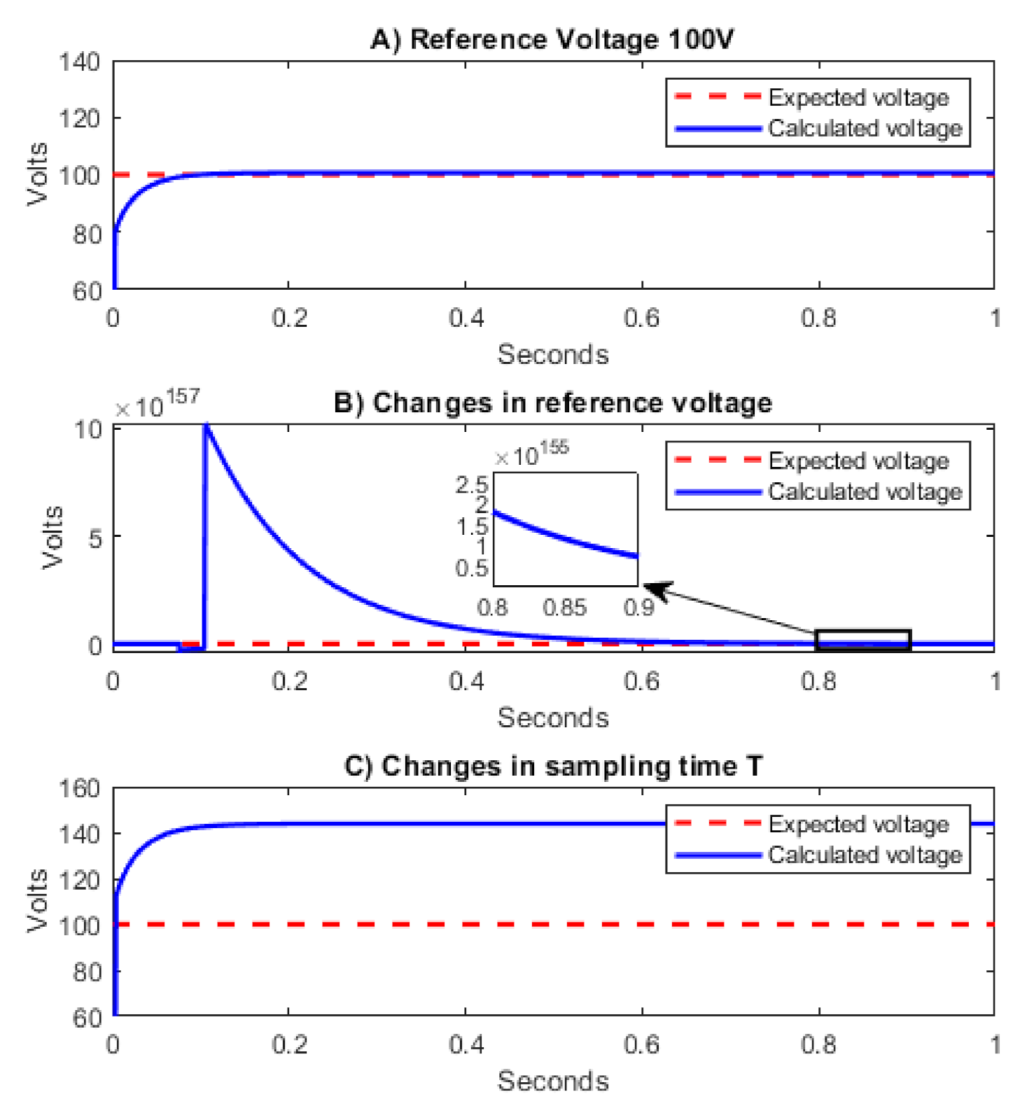
6.1. Changes in Reference, Sampling Time, and Input Variables

To test the proposed method, the following fixed values are taken in the following simulation: L = 12   m H , R L = 220   Ω , C = 500   μ F , changing the sampling time T = 10   μ s taking as reference voltage 120 V, with fixed P and R previously defined, the adjustment value in our method is K = 7.45 . Additionally, the input voltage to the boost converter is a determined variable. The above test the robustness of the control method. Such input voltage changes are from 50 V to 70 V, from 70 V to 110 V, and from 110 V to 90 V. The simulation results are shown in Figure 3.
Figure 3 shows that the stability of the boost converter is preserved in the event of voltage changes, with a maximum percentage error ξ 0.041 % and is reached when v 1 = 50 V, Figure 3a shows the calculated current and expected current, Figure 3b the controlled output voltage reaches the changes in the reference voltage, Figure 3c the duty cycle values calculated by the inverse control law, and Figure 3d the input voltage changes. On the other hand, it is also important to consider changes in the load, since in electrical systems the load is rarely constant over time. To analyze the stability before these changes, consider the values L = 12   m H , C = 500   μ F , T = 10   μ s , with a reference voltage of 120 V and an input voltage of 80 V. The changes in the load are from 50   Ω to 100   Ω , from 100   Ω to 200   Ω , and from 200   Ω to 300   Ω . The results are presented in Figure 4, showing ξ values around 0.02 %.
The stability of the output voltage is maintained due to the inverse optimal control by the tuning of the K coefficient under different changes in the load.
Finally, the proposed method is used to stabilize the system against various changes in the reference. This is achieved by assigning a variable adjustment for each reference value as follows:
v r e f 1 v r e f 2 v r e f 3 v r e f n K 1 K 2 K 3 K n
Given the fixed values L = 12   m H , R L = 220   Ω , C = 500   μ F , v 1 = 80   V , and the following changes in the reference voltage ranging from 100 V to 120 V, from 120 V to 140 V, and from 140 V to 130 V. The adjustment coefficients K s for each reference voltage K 100 V = 10.95 ,   K 120 V = 7.45 ,   K 130 V = 6.27 , and K 140 V = 5.1 . The respective simulation results are shown in Figure 5.
In Figure 5b, the stability of the boost converter can be observed under changes in the reference voltage due to the proposed coefficients, and Table 1 shows the obtained percentage errors. It is important to emphasize that the four changes in the voltage reference are achieved in a period of 2 s. A period in which the changes and the scope of the desired objectives are appreciated.
Furthermore, considering the found coefficients for the changes in the voltage reference, the possibility of a correspondence between the reference voltages and the found coefficients are analyzed, obtaining that there is a linear type relation taken from three of the coefficients. The linear function is as follows.
K = 0.117 v r e f + 21.48
This relation is important since an adjustment coefficient is found, which ensures stability over a wider range for different reference voltage values and it will make our control much more robust. The approximation is better in the interval of [120 V, 140 V] since the coefficients of these were the ones that best adjusted to a linear adjustment, otherwise, the coefficient K 100 V was the one that had a greater dispersion in this adjustment, therefore an increase in error may be its consequence.
Equation (15) can be rewritten as
u k * = 0.117 v r e f + 21.48 R + 1 2 g T x k P g x k 1 g T x k P f x k x δ , k + 1
Figure 6 shows the implementation of the inverse optimal control using Equation (17), taking the same fixed variables of Figure 5, with changes in the voltage reference from 105 V to 115 V, from 115 V to 150 V, and from 150 V to 125 V. Therefore, it has been possible to extend the operating range of the inverse optimal control, without the need to search for the K s coefficients for different reference voltage values, where the highest value of ξ is 0.4% when the voltage reference is equal to 150 V.

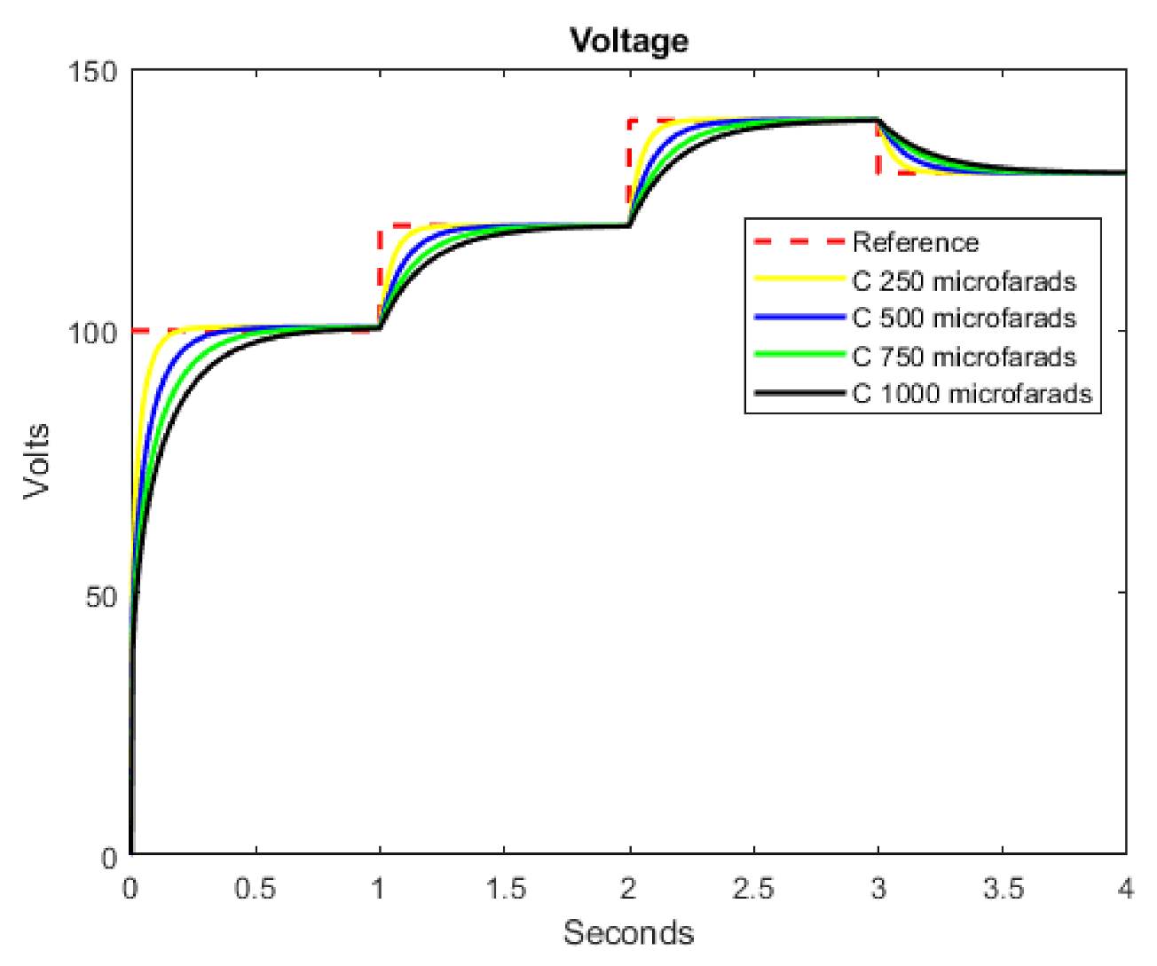
6.2. Robustness Analysis

To test the robustness of the model, the boost converter is subjected to changes in the parameters of the system Equations (1) and (2). These changes may be due to the heating of the boost converter components. As the physical components of the boost converter are fixed, variations in capacitance and inductance upon heating are small. Therefore, in this work, changes in capacitance and inductance are addressed, which will show the robustness of the control. That is, changes are made in the capacitance and inductance that show an operating range or the operating limits before their changes, which satisfy that ξ < ε in all cases. Therefore, if ξ < ε is not met, the new proposed methodology will be applied to adjust the control.
Given the fixed values L = 12   m H , R L = 220   Ω , v 1 = 80   V , Figure 7 shows the behavior of the impulse to changes in capacitance based on a capacitance of C = 500   μ F with an increase in capacitance of 50% and 100%, and a decrease in capacitance of 50%, in addition to changes in the voltage reference. Table 2 shows the error percentage according to the reference voltage, obtaining a maximum error percentage of 0.62%.
Table 2 shows the maximum percentages of the error, and these are reached when the reference voltage is 100 V, which is because the control Equation (22) was obtained based on the coefficients K s corresponding to 120 V and 140 V. On the other hand, the changes presented by capacitance generate errors of less than 1% in all simulations (Percentage error of Table 2 is 0.1777%).
Figure 8 shows the behavior of the boost converter under changes in the inductance. The base inductance is L = 12   m H , where changes in inductance can be seen ranging from 8% with L = 11   m H , and L = 13   m H , to 20% with values of L = 9.5   m H , and 16.6% with L = 14   m H . Where a maximum error of 2.34% is reached according to the voltage reference.
Table 3 provides the percentages of the error due to changes in the voltage reference and changes in the inductance, it shows that the maximum percentages of error are reached when the inductance has the values L = 10   m H and L = 14   m H , with an average percentage error of the table of 0.866%. In the same way, the values, in general, are higher when the reference value is equal to 100 V, this last behavior is due to the adjustment of the curve already mentioned.
Given that our percentage error is ξ > ε in several cases in Table 3, a new adjustment is made from these values. Although a methodology has been proposed to be able to find the coefficient K that fits each combination in such a way that ξ < ε and is also minimal, the new search is as follows:
K L i = 0.117 v r e f + 21.48 + γ L i
Where K L i   is the adjustment coefficient due to changes in inductance L i and changes in the voltage reference v r e f . γ L i is the adjustment coefficient that depends on the inductance. The graph of the coefficients γ L i can have any form.
The objective is to find the γ L i for the inductance values L = 10   m H and L = 14   m H that comply with ξ < ε , with these coefficients a new linear fit is proposed for γ L i , whose equation is given by
γ L = 1.25 L 14.7
Substituting Equation (24) in Equation (23), the following is obtained:
K = 0.117 v r e f + 1.25 L + 6.78
This new equation fits into an inductance interval of 10   m H ,   14   m H . Table 4 shows the combinations from Table 2 using Equation (25) to obtain the K s . Where the average percentage error in Table 4 is 0.2369%.
The average percentage error in Table 4 decreases by approximately 72%, also ξ < ε , for all shocks. On the other hand, ξ is sacrificed a bit, since in some cases, the percentage error increases due to the new adjustment. On the other hand, this new adjustment provides a more robust control of the output voltage of the system, since ξ < ε is achieved with a single adjustment equation in the event of changes in the input variables and in the system parameters.

6.3. Analysis for Different Voltage Reference Changes

Figure 9 shows simulations under changes in inductance similar to Figure 8, Figure 9a shows the voltage outputs of the boost converter without the adjustment of Equation (25) and after the linear fit, obtaining better approximations even in a range inductance that is outside the proposed setting. At Figure 9b shows the voltage output of the boost converter without linear fit, but with two different types of changes in the reference voltage. On the one hand, an order is shown that has an increase in the totally increasing reference voltage, and in turn, an order in which there is an increase and decrease in the reference voltage, obtaining better behavior in the output voltage when the changes are monotonically growing. In this way, it is important to consider the order of changes in the voltage references, since this can affect the stability of the system. On the other hand, the linear fit obtained with the new methodology proposed in this work also solves this problem.

7. Conclusions

In this paper, a new inverse optimal control for a boost converter has been developed. Besides, a new method to tune the inverse optimal control was proposed. Such a method was tested for changes in the reference voltage, also, it was proved that said tuning of the control method has a good response under changes in the input voltage and in the load. Furthermore, based on the results, it can be deduced that the method can help to find a relation of the proposed K s for the boost converter, subject to changes in the input variables and the given reference, in addition to changes in the system parameters. In our case, there is a linear type relation, to expand the robustness of the model in the face of changes in the voltage reference, which ensures the stability of our system. Taking the amplitude of each interval and comparing the lower and upper limits of each variable, at which the new control methodology was tested in our system. Said coefficient of linear adjustment was able to damp, an amplitude of 50 V for the reference voltage, corresponding to a change of 50%. An amplitude of 250 Ω corresponding to a 500% change in load. It was tested with an input voltage variation of 120%. For capacitance, an amplitude of 5 m H corresponding to a change of 55% and for inductance an amplitude of 750   μ F corresponding to changes of up to 300%. Whose system stability was preserved, with an error of less than 1% according to the voltage reference. Simulation results probe the effectiveness of our proposed control methodology.

Author Contributions

Conceptualization, M.V.-R. and A.C.-M.; methodology, K.J.G.-T.; software, M.V.-R.; validation, M.V.-R., K.J.G.-T., and A.C.-M.; formal analysis, M.V.-R. and K.J.G.-T.; investigation, M.V.-R.; resources, A.C.-M.; data curation, M.V.-R.; writing—original draft preparation, M.V.-R.; writing—review and editing, A.C.-M.; visualization, A.C.-M.; supervision, A.C.-M.; project administration, A.C.-M.; funding acquisition, A.C.-M. All authors have read and agreed to the published version of the manuscript.

Funding

This research received no external funding.

Institutional Review Board Statement

Not applicable.

Informed Consent Statement

Not applicable.

Data Availability Statement

All data are specified in the article.

Acknowledgments

The first author thanks Consejo Nacional de Ciencia y Tecnología (CONACyT) for the scholarship awarded with number 261687 for the doctorate studies in Water and Energy, and to the University of Guadalajara (México) for providing me with the space and conditions to develop this work.

Conflicts of Interest

The authors declare no conflict of interest.

Abbreviations

CLFControl Lyapunov Function
PWMPulse Width Modulated Signal
HJBHamilton–Jacobi–Bellman
PSOParticle Swarm Optimization
GAGenetic Algorithm
PIProportional–Integral Control
PIDProportional–Integral–Derivative Control

Nomenclature

v 0 Capacitor voltage
i L Inductor current
v 1 Input voltage
L Inductance of the inductor
C Capacitance of the capacitor
R L A resistance
U Is the signal control ( U = 0 U = 1 )
u Is the duty cycle
k Time
x k State of the system at time k
x k + 1 State of the system at time k + 1
u k Is the input corresponding to the control signals at time k
f It is a function of the state of the system
g It is a function of the state of the system
J z k Cost functional
z k Tracking error
l z k Is a positive semidefinite function
P Is a real symmetric positive definite weighting matrix
R Is positive definite
x δ , k The desired trajectory for x k
V x k Lyapunov function
V z k Lyapunov function
H z k ,   u k Discrete-time Hamiltonian
u k * The optimal control law to achieve trajectory tracking
K Control setting constant
ξ Percentage error
ε Tolerance error
v r e f Reference voltage
x 1 , k Output current at time k
x 2 , k Output voltage at time k

References

  1. Güler, N.; Irmak, E. Design, Implementation and Model Predictive Based Control of a Mode-Changeable DC/DC Converter for Hybrid Renewable Energy Systems. ISA Trans. 2020. [Google Scholar] [CrossRef]
  2. Palomba, V.; Borri, E.; Charalampidis, A.; Frazzica, A.; Cabeza, L.F.; Karellas, S. Implementation of a Solar-Biomass System for Multi-Family Houses: Towards 100% Renewable Energy Utilization. Renew. Energy 2020, 166, 190–209. [Google Scholar] [CrossRef]
  3. Antwi, S.H.; Ley, D. Renewable Energy Project Implementation in Africa: Ensuring Sustainability through Community Acceptability. Sci. Afr. 2021, 11, e00679. [Google Scholar] [CrossRef]
  4. Upadhyay, P.; Kumar, R. A High Gain Cascaded Boost Converter with Reduced Voltage Stress for PV Application. Sol. Energy 2019, 183, 829–841. [Google Scholar] [CrossRef]
  5. Fathabadi, H. Novel High Efficiency DC/DC Boost Converter for Using in Photovoltaic Systems. Sol. Energy 2016, 125, 22–31. [Google Scholar] [CrossRef]
  6. Cucuzzella, M.; Lazzari, R.; Trip, S.; Rosti, S.; Sandroni, C.; Ferrara, A. Control Engineering Practice Sliding Mode Voltage Control of Boost Converters in DC Microgrids. Control Eng. Pract. 2018, 73, 161–170. [Google Scholar] [CrossRef]
  7. Rahimi, M. Modeling, Control and Stability Analysis of Grid Connected PMSG Based Wind Turbine Assisted with Diode Rectifier and Boost Converter. Int. J. Electr. Power Energy Syst. 2017, 93, 84–96. [Google Scholar] [CrossRef]
  8. Slah, F.; Mansour, A.; Hajer, M.; Faouzi, B. Analysis, Modeling and Implementation of an Interleaved Boost DC-DC Converter for Fuel Cell Used in Electric Vehicle. Int. J. Hydrog. Energy 2017, 42, 28852–28864. [Google Scholar] [CrossRef]
  9. Wen, H.; Su, B. Hybrid-Mode Interleaved Boost Converter Design for Fuel Cell Electric Vehicles. Energy Convers. Manag. 2016, 122, 477–487. [Google Scholar] [CrossRef]
  10. Xu, L.; Hong, P.; Fang, C.; Li, J.; Ouyang, M.; Lehnert, W. Interactions between a Polymer Electrolyte Membrane Fuel Cell and Boost Converter Utilizing a Multiscale Model. J. Power Sources 2018, 395, 237–250. [Google Scholar] [CrossRef]
  11. Sobrino-Manzanares, F.; Garrig, A. ScienceDirect Multi-Switch Synchronous Boost Converter for Fuel Cell Applications. Int. J. Hydrog. Energy 2015. [Google Scholar] [CrossRef]
  12. Forouzesh, M.; Siwakoti, Y.P.; Gorji, S.A.; Blaabjerg, F.; Lehman, B. Overview Step-Up DC. DC Converters: A Comprehensive Review of Voltage-Boosting Techniques. IEEE Trans. Power Electron. 2017, 32, 9143–9178. [Google Scholar] [CrossRef]
  13. Dash, S.S.; Nayak, B. Control Analysis and Experimental Verification of a Practical Dc–Dc Boost Converter. J. Electr. Syst. Inf. Technol. 2015, 2, 378–390. [Google Scholar] [CrossRef] [Green Version]
  14. Nouri, A.; Salhi, I.; Elwarraki, E.; El Beid, S.; Essounbouli, N. DSP-Based Implementation of a Self-Tuning Fuzzy Controller for Three-Level Boost Converter. Electr. Power Syst. Res. 2017, 146, 286–297. [Google Scholar] [CrossRef]
  15. Abdelmalek, S.; Dali, A.; Bakdi, A.; Bettayeb, M. Design and Experimental Implementation of a New Robust Observer-Based Nonlinear Controller for DC-DC Buck Converters. Energy 2020, 213, 118816. [Google Scholar] [CrossRef]
  16. Cheng, Z.; Li, Z.; Li, S.; Gao, J.; Si, J.; Das, H.S.; Dong, W. A Novel Cascaded Control to Improve Stability and Inertia of Parallel Buck-Boost Converters in DC Microgrid. Int. J. Electr. Power Energy Syst. 2020, 119, 105950. [Google Scholar] [CrossRef]
  17. Qingfeng, L.; Zhaoxia, L.; Jinkun, S.; Huamin, W. A Composite PWM Control Strategy for Boost Converter. Phys. Procedia 2012, 24, 2053–2058. [Google Scholar] [CrossRef] [Green Version]
  18. Siddhartha, V.; Hote, Y.V.; Saxena, S. Non-Ideal Modelling and IMC Based PID Controller Design of PWM DC-DC Buck Converter. IFAC-PapersOnLine 2018, 51, 639–644. [Google Scholar] [CrossRef]
  19. Dinniyah, F.S.; Wahab, W.; Alif, M. Simulation of Buck-Boost Converter for Solar Panels Using PID Controller. Energy Procedia 2017, 115, 102–113. [Google Scholar] [CrossRef]
  20. Repecho, V.; Biel, D.; Olm, J.M.; Fossas, E. Robust Sliding Mode Control of a DC/DC Boost Converter with Switching Frequency Regulation. J. Frankl. Inst. 2018, 355, 5367–5383. [Google Scholar] [CrossRef]
  21. Coronado-Mendoza, A.; Gurubel-Tun, K.J.; Zúñiga-Grajeda, V.; Domínguez-Navarro, J.A.; Artal-Sevil, J.S. Variable Frequency Control of a Photovoltaic Boost Converter System with Power Quality Indexes Based on Dynamic Phasors. IFAC-PapersOnLine 2018, 51, 180–185. [Google Scholar] [CrossRef]
  22. Dancholvichit, N.; Kapoor, S.G.; Salapaka, S.M. Temperature Regulation for Thermoplastic Micro-Forming of Bulk Metallic Glass: Robust Control Design Using Buck Converter. J. Manuf. Process. 2020, 56, 1294–1303. [Google Scholar] [CrossRef]
  23. Seguel, J.L.; Seleme, S.I. Robust Digital Control Strategy Based on Fuzzy Logic for a Solar Charger of VRLA Batteries. Energies 2021, 14, 1001. [Google Scholar] [CrossRef]
  24. Vega Pérez, C.J.; Alzate Castaño, R. Control Óptimo Inverso Como Alternativa Para La Regulación de Un Convertidor DC-DC Elevador. Rev. Tecnura 2015, 19, 65. [Google Scholar] [CrossRef] [Green Version]
  25. Vega, C.; Alzate, R. Inverse Optimal Control on Electric Power Conversion. In Proceedings of the 2014 IEEE International Autumn Meeting on Power, Electronics and Computing (ROPEC), Ixtapa, Mexico, 5–7 November 2014. [Google Scholar] [CrossRef]
  26. Sanchez, E.N.; Ornelas-Tellez, F. Discrete-Time Inverse Optimal Control for Nonlinear Systems; CRC Press: Boca Raton, FL, USA, 2017; ISBN 9781466580886. [Google Scholar]
  27. Alsmadi, Y.M.; Utkin, V.; Haj-ahmed, M.A.; Xu, L. Sliding Mode Control of Power Converters: DC/DC Converters. Int. J. Control 2018, 91, 2472–2493. [Google Scholar] [CrossRef]
  28. Yang, T.; Liao, Y. Discrete Sliding Mode Control Strategy for Start-up and Steady-State of Boost Converter. Energies 2019, 14, 2990. [Google Scholar] [CrossRef] [Green Version]
  29. Vega Pérez, C.; Alzate Castaño, R. Control Óptimo Inverso Para Sistemas No Lineales En Tiempo Continuo. Respuestas 2014, 19, 13–18. [Google Scholar] [CrossRef]
  30. Do, K.D. Inverse Optimal Control of Stochastic Systems Driven by Lévy Processes. Automatica 2019, 107, 539–550. [Google Scholar] [CrossRef]
  31. Ornelas, F.; Sanchez, E.N.; Loukianov, A.G. Discrete-Time Inverse Optimal Control for Nonlinear Systems Trajectory Tracking. Proc. IEEE Conf. Decis. Control 2010, 4813–4818. [Google Scholar] [CrossRef]
  32. Sakly, M.; Sakly, A.; M’Sahli, F. Inverse Optimal Control of Switched Discrete Non Linear Systems Based on Control Lyapunov Function and Genetic Algorithm. In Proceedings of the 16th International Conference on Sciences and Techniques of Automatic Control and Computer Engineering (STA 2015), Monastir, Tunisia, 21–23 December 2015. [Google Scholar] [CrossRef]
  33. Ornelas-Tellez, F.; Sanchez, E.N.; Loukianov, A.G.; Rico, J.J. Robust Inverse Optimal Control for Discrete-Time Nonlinear System Stabilization. Eur. J. Control 2014, 20, 38–44. [Google Scholar] [CrossRef]
  34. El-Hussieny, H.; Abouelsoud, A.A.; Assal, S.F.M.; Megahed, S.M. Adaptive Learning of Human Motor Behaviors: An Evolving Inverse Optimal Control Approach. Eng. Appl. Artif. Intell. 2016, 50, 115–124. [Google Scholar] [CrossRef]
  35. Lastire, E.A.; Sanchez, E.N.; Alanis, A.Y.; Ornelas-Tellez, F. Passivity Analysis of Discrete-Time Inverse Optimal Control for Trajectory Tracking. J. Frankl. Inst. 2016, 353, 3192–3206. [Google Scholar] [CrossRef]
  36. Zhang, Y.; Mohammadpour Shotorbani, A.; Wang, L.; Mohammadi-Ivatloo, B. Enhanced PI Control and Adaptive Gain Tuning Schemes for Distributed Secondary Control of an Islanded Microgrid. IET Renew. Power Gener. 2021, 1–11. [Google Scholar] [CrossRef]
  37. Lhachemi, H.; Saussié, D.; Zhu, B. Hidden Coupling Terms Inclusion in Gain-Scheduling Control Design: Extension of an Eigenstructure Assignment-Based Technique. IFAC-PapersOnLine 2016, 49, 403–408. [Google Scholar]
  38. Kersten, J.; Rauh, A.; Aschemann, H. Interval Methods for Robust Gain Scheduling Controllers. Granul. Comput. 2020, 5, 203–216. [Google Scholar] [CrossRef]
  39. Awad, O.A.; Salim, I.L. Fuzzy PID Gain Scheduling Controller for Networked Control System. Iraqi J. Sci. 2021, 210–216. [Google Scholar] [CrossRef]
  40. Bhukya, L.; Annamraju, A.; Srikanth, N. Robust Frequency Control in a Wind-Diesel Autonomous Microgrid: A Novel Two-Level Control Approach. Renew. Energy Focus 2021, 36, 21–30. [Google Scholar] [CrossRef]
Figure 1. Diagram of a boost converter.
Energies 14 02507 g001
Figure 2. (A) Implementation of inverse optimal control, (B) change in reference voltage, (C) change in sampling time T .
Energies 14 02507 g002
Figure 3. (A) Shows current behavior, (B) boost converter output voltage, (C) duty cycle, and (D) input voltage changes.
Energies 14 02507 g003
Figure 4. (A) Shows current behavior, (B) boost converter output voltage, (C) duty cycle, and (D) changes in load.
Energies 14 02507 g004
Figure 5. (A) Shows current behavior, (B) boost converter output voltage under changes in reference voltage, (C) duty cycle, and (D) input voltage.
Energies 14 02507 g005
Figure 6. Boost converter under changes in the voltage reference, using the K’s coefficients of the linear adjustment function.
Energies 14 02507 g006
Figure 7. Output voltage of a boost converter under changes in reference voltage and capacitance.
Energies 14 02507 g007
Figure 8. Output voltage of a boost converter under changes in reference voltage and inductance.
Energies 14 02507 g008
Figure 9. Comparison of the output voltage under changes in the inductance and the reference voltage, (A) with and without linear fit, (B) without linear fit, with two different accommodations of changes in inductance.
Energies 14 02507 g009
Table 1. Percentage errors for each reference voltage.
Reference Voltage100 V120 V140 V130 V
Error   % 0.250.110.020.06
Table 2. Percentage of error in the output voltage due to changes in capacitance.
Error   %  
Reference Voltage
Capacitance (Microfarads)100120140130
2500.62060.00610.13390.0029
5000.61740.00540.13270.0035
7500.57970.01400.11280.0154
10000.40450.09900.02960.0647
Table 3. Percentage of error in the output voltage due to changes in the inductance.
Error   %
Reference Voltage
Inductance (Millihenries)100120140130
101.51551.49421.03581.3005
110.38510.70050.41890.611
120.61740.00540.13270.0035
131.52110.64350.63380.5602
142.34631.2281.09491.071
Table 4. Percentage error in the output voltage due to changes in the inductance.
Error   %
Reference Voltage
Inductance (Millihenries)100120140130
100.104730.185330.739340.12719
110.185140.194620.189060.08304
120.447030.141090.030920.14510
130.681330.062050.116660.14156
140.890510.025860.139870.10738
Publisher’s Note: MDPI stays neutral with regard to jurisdictional claims in published maps and institutional affiliations.

