Diagnostic Row Reasoning Method Based on Multiple-Valued Evaluation of Residuals and Elementary Symptoms Sequence

Abstract

The paper analyses the research problem of conducting diagnostic reasoning for dynamic objects to eliminate the possibility of formulating false diagnoses resulting from different delays of the symptoms related to a particular fault while simultaneously striving to obtain high distinguishability. The research aimed to develop a new diagnostic inference method robust to symptom delays and characterised by high accuracy of generated diagnosis. Known methods ensuring the correctness of inference in the case of symptom delays but at the cost of reducing distinguishability of faults have been characterised. A new inference method was developed, which uses the three-valued residual evaluation and knowledge regarding elementary symptom sequences. A formal description of the diagnosing system and the proposed method are given. The method of obtaining the knowledge about the order of symptoms based on a cause-and-effect graph and was characterised. The method’s effectiveness was presented in simulation studies on the example of diagnosing a set of serially connected tanks. The comparison of the fault distinguishability obtained using the proposed method and other approaches illustrates the new method’s advantages.

1. Introduction

Over the last twenty years, there has been a rapid development of fault diagnosis methods derived from the theory of modelling and identification and artificial intelligence techniques. The broadest description of these methods can be found in books [1,2,3,4,5,6,7]. A valuable source of knowledge are the materials of the IFAC Symposium on Fault Detection, Supervision and Safety for Technical Processes SAFEPROCESS and Workshop on the Principles of Diagnosis DX.

In diagnostics of complex dynamic objects covering, e.g., processes in chemical, petrochemical, power, and food industries, etc., there are many problems and restrictions [8] which are of minor importance in the diagnostics of devices, machines, and processes of small scale. These problems must be addressed and resolved so that the diagnostic system is adequately robust and able to recognise the emerging faults effectively.

One such problem is delays of the symptoms of faults. The object of diagnosis is a dynamic system. Therefore, from the moment of fault occurrence to the moment of observing a measurable symptom, a certain time passes depending on the dynamic properties of the tested element of the process and on the detection algorithm. The same fault is detected after different periods by different diagnostic tests using partial models of the process. When the fault isolation algorithm does not have embedded mechanisms making reasoning resistant to symptom delays, the false diagnoses may be generated. The problem has been analysed in the following studies [9,10,11,12,13,14,15].

The notation of the relationship between faults and symptoms may take different forms. However, it does not consider the dynamics of the symptoms. The exception is the notation of residuals in the internal form. The most commonly used is a Binary Diagnostic Matrix (BDM) [5,11], also referred to as the structure of residual sets [3], Boolean decision table [2], coding set [6,16], Boolean fault signature matrix [14,17,18] and the effect of the faults on the residuals [1]. The reasoning about faults based on BDM is conducted in two ways:

• Column Reasoning is used in the Fault Detection and Isolation (FDI) environment, where the BDM columns correspond to the fault signatures.
• Row Reasoning is used in a DX environment (DX comes from the word diagnosis. This abbreviation is used to describe the group of formal logic and artificial intelligence specialists dealing with the development of diagnostic methods.) where the rows of BDM define conflict sets corresponding to the sets of faults detected by particular tests [19].

IF-THEN rules, logical functions and fault trees [5,20] are also applied for the notation of the fault-symptom relation. Another solution is the Fault Isolation System (FIS) [5,11,21], which uses multivalent evaluations of the residuals.

All of these manners of mapping are of a static character, whereas during diagnosing in real-time, the same fault is detected after a different time by different diagnostic signals. Thus, if we examine the set of diagnostic signals detecting a particular fault, then in a particular moment after the occurrence of the fault, only part of these signals takes the values, which are symptoms of the fault. After a certain time, the values indicating faults will be established on the outputs of all these signals. Not considering the dynamics of the formation of symptoms may lead to the generation of false diagnoses [11,14].

For Large Scale Systems (LSS), the problem then arises of how to conduct diagnostic reasoning in the situation of delay of the emergence of symptoms in such a way that the diagnoses are correct, and the distinguishability of the faults is possibly high. Known solutions do not guarantee this. In the case of LSS, there are significant limitations related to the scale of the system: a very high number of possible faults, a large set of measuring devices and implemented detection algorithms, etc. Acquisition of knowledge about the fault-symptom relationship is only possible on the basis of expert knowledge. Modelling methods that consider the impact of faults, as well as learning methods, are not useful. Modelling with the influence of the faults is very difficult, costly and, in many cases, even impossible [22]. This means that the internal form of the residuals is unknown. Learning methods [4,5,23,24] require knowledge of measurement data characterising all states of the process that should be recognised, therefore, the normal state of the process and the states with faults. Collecting measuring data for all emergency states is impossible [8,25]. Particular emergency states rarely occur, while their first occurrence should already be recognised.

The paper presents a new method of diagnostic reasoning that prevents the formation of false diagnoses due to different delays of the symptoms of the same fault. It allows for obtaining a high distinguishability of the faults compared to other methods resistant to the delay of the symptoms. The awareness of the internal form of the residuals is not necessary. The uniqueness of this method lies in using heuristic knowledge about the elementary sequences of symptom formation, together with a multivalent evaluation of the residuals. This expands the method presented in [15]. The proposed method is intended to diagnose complex industrial processes. Only the passive approach is considered, as opposed to the active approach [26,27].

The structure of the paper is as follows: in Section 2, the properties and restrictions of the known solutions ensuring the correct functioning of the diagnostic process when symptoms are delayed are discussed. A formal description of the knowledge about the diagnosed process is given in Section 3. This description includes a model of faults-symptoms relationship (Section 3.1) and a notation of the knowledge about elementary symptoms sequences (Section 3.2). Section 4 discusses the methods of acquiring knowledge about the symptom forming order based on the cause and consequence graph of the process. A new method of diagnostic reasoning which prevents the formation of false diagnoses as a consequence of different delays of symptoms of the same fault, and in many cases allows for increasing the distinguishability of the fault, is included in Section 5. Section 6 serves as an example of applying the method and comparing the distinguishability of the faults achieved by the new method with other known solutions. Section 7 summarises the results of the study.

2. Related Works

The complete knowledge about the diagnosed object is given by its models, e.g., state equations acknowledging not only the influence of the inputs but also the faults on the outputs. The values of residuals are explicitly dependent on the faults. In linear models, their computational and internal forms are determined [2,3]. Methods within that group provide the best opportunities to use the knowledge about the dynamics of symptoms emergence.

In [28] a method of designing the so-called sequential residuals has been given for linear systems on the basis of the knowledge of internal forms of the residuals. It provides an opportunity to design distinguishable sequences for faults undistinguishable by primary residuals. For specific faults, sequences of symptoms may be obtained that provide the required properties, such as concurrent symptoms, symptoms in any order, and symptoms displaced towards each other by a desired delay. However, this method cannot be applied when the internal form of the residuals is unknown, which usually occurs in the diagnostics of industrial processes (industrial FDI).

The gist of the proposed algorithm of fault isolation is the use of multivalent evaluation of the residuals and knowledge about the order of fault symptoms. Symptom forming order has been analysed in numerous papers. Temporal information can be included in the Signed Directed Graph (SDG), as shown in [29,30]. In these papers, attention is paid to the fact that the path of fault propagation in SDG must agree with the recorded symptoms sequences. Another approach is applying Temporal Causal Graph to transcend system in diagnostics [10,31,32,33,34]. Temporal information has also been included in discrete event systems [13,35,36].

A few ways of protecting the fault isolation algorithm against generating false diagnoses due to the delays of the emergence of the symptoms are known at the moment. The basic solution is by only using symptoms during reasoning. Zero values of signals are ignored, as they may change their value due to possible delays in response to faults [18]. This kind of approach is used in the DX environment. A similar solution is symptom-based reasoning [12]. However, during the reasoning, ignoring the diagnostic signals with zero value will reduce the faults distinguishability.

Another solution is diagnosing while taking into account the maximum delay time of the symptoms defined for particular isolation algorithms [11]. This ensures correct reasoning as the diagnoses are formulated just after determining the symptoms. The obtained distinguishability of faults is the same as the one obtained on the basis of the binary diagnostic matrix, although the time of diagnosing is rather long.

The approach using minimal and maximal delay times of the symptoms in diagnostic algorithms of a given fault [13] allows for increasing the distinguishability of faults compared to the above two methods. It is, however, very difficult in practice due to the difficulties in estimating minimal and maximal values of the delay times of the symptoms. A similar approach, proposed in [14], characterises symptom apparition times (delays) through the fuzzy time interval in the form of a trapezoid. This work, to improve the efficiency of the entire fault diagnosis system, utilises the size of the residual value and residual signs, the sensitivity of a residual expression concerning a certain fault, the time pattern of fault signal occurrence, and the order of fault signal occurrence. Obtaining data on the time profile of the symptom emergence and the sensitivity of the residuum to fault requires either the knowledge of the internal form of the residuum or the possibility of recording measurement data in states with faults. This is unrealistic in the case of LSS.

In [15], a method of diagnosing is presented where the knowledge on a binary diagnostic relation is used and heuristic knowledge (usually incomplete) about the symptoms forming order. It is called SSFI—symptoms sequence fault isolation. This algorithm prevents diagnostic errors related to delays in the emergence of the symptoms. It allows for increasing the distinguishability of faults concerning the algorithm of symptom-based reasoning. The more complete the knowledge of the relations between delays of symptoms, the greater the increase in distinguishability.

This paper is a generalisation and extension of the above concept. The extension includes the use of FIS to describe the relationship between faults and symptoms instead of BMD and accepting multivalent evaluation of residuals. The multivalent residuals evaluation allows a significant reduction of incorrect diagnoses resulting from the binary evaluation of the residuals and the compensation of the fault’s impact on the values of the residuals. In the new approach, by reducing false diagnoses resulting from symptom delays, a further increase in the robustness of the fault isolation algorithm is achieved. A way of defining some symptoms forming order on the basis of a-graph of a process is also presented in the paper.

3. Formal Notation of Knowledge on a Diagnosed Object

3.1. Relation between Faults and the Values of Diagnostic Signals

Diagnostic signals result from the binary or multivalent evaluation of the residuals calculated on the basis of the models to detect faults. They can also be the outputs of heuristic tests. For the diagnosis, it is necessary to know the representation of the space of diagnostic signals’ values:

$$S=\left\{s_j:j=1,2,\dots ,J\right\}$$

(1)

in the space of faults:

$$F=\left\{f_k:k=1,2,\dots ,K\right\}.$$

(2)

The FIS was defined in [21] in the form of the following four:

$$FIS=\langle F,S,V_S,q\rangle .$$

(3)

where:

• $F$—a finite set of faults;
• $S$—a finite set of diagnostic signals;

$$V_S={{\displaystyle \cup }}_{s_j\in S}{V}_j—\mathrm{a} \mathrm{set} \mathrm{of} \mathrm{diagnostic} \mathrm{signals} \mathrm{values};$$

(4)

• $V_j$—a set of the values of j-th diagnostic signal,
• $q$—representation:

$$q:F\times S\to \varphi \left(V_S\right)$$

(5)

assigning a subset of the values of diagnostic signals to each element of the Cartesian product $F\times S$:

$$q(f_k,s_j)\equiv V_{kj}\subset V_j,$$

(6)

which can receive this signal when $f_k$ fault occurs.

Furthermore, let us assume that the value of a diagnostic signal $s_j=0$ corresponds to a no-faults state, and the other values are symptoms of the faults.

FIS is then a table defining model values of diagnostic signals for the particular faults. It is a generalisation of the binary diagnostic matrix. If the set of all values of diagnostic signals is identical and equal to $V_S=\left\{0,1\right\},$ and $q\left(f_k,s_j\right)$ is a singleton, FIS is simplified to a binary diagnostic matrix. Significant extensions of FIS concerning the binary diagnostic matrix are as follows:

• Each diagnostic signal may have an individual set of its values $V_j$.
• $V_j$ set of the j-th value of diagnostic signal includes the value of 0 and the values that differ from 0, which are the fault symptoms.
• $q\left(f_k,s_j\right)$ element of a Cartesian product $F\times S$ is in a general case, a subset of the values $V_{kj}\subset V_j$, which may be taken by a j-th diagnostic signal when the k-th fault appears.

FIS provides a greater distinguishability of faults when compared to the binary diagnostic matrix, what has been presented in [21,37,38].

Suppose that, for the analogy from BDM we present a graphical representation of FIS in the form of a table (Example 1,

Table 1. Example of Q.

S/F	${\mathit{f}}_1$	${\mathit{f}}_2$	${\mathit{f}}_3$	${\mathit{f}}_4$	${\mathit{f}}_5$	${\mathit{f}}_6$	${\mathit{V}}_{\mathit{j}}$
${\mathit{s}}_{\mathbf{1}}$	1	0	1	0	0	1	0, 1
${\mathit{s}}_{\mathbf{2}}$	0	−1	0	+1	−1	0	0, −1, +1
${\mathit{s}}_{\mathbf{3}}$	−1	+1	−1, +1	0	+1	+1	0, −1, +1
${\mathit{s}}_{\mathbf{4}}$	0	1, 2	1	0	1, 2	1, 2	0, 1, 2
${\mathit{s}}_{\mathbf{5}}$	+1	0	+1	+1	0	−1, +1	0, −1, +1

), the rows of which correspond to $s_j\in S$ diagnostic signals, and the columns to $f_k\in F$ faults. In such a case, the signature of the fault corresponds to the FIS column and is described by the following dependence:

$$Q\left(f_k\right) = {\left[V_{k1},V_{k2},\dots ,V_{kJ}\right]}^T.$$

(7)

The above notation of the relation between faults and diagnostic signal values is especially useful for the three-valued evaluation of residual values, as it enables the residual sign to be considered. However, this form is more general, which allows for the interpretation of diagnostic signals obtained by other methods, e.g., visual. If the fault symptoms are related to the colours of the flame, the FIS allows to express this relationship for, e.g., four distinct colours: yellow, orange, red and purple.

Classical signature-based reasoning is realised on the basis of all diagnostic signals. Diagnosis is formulated as a result of the comparison of the obtained values of diagnostic signals with the signature of the state including only zeros and signatures of the particular faults (7). The diagnosis indicates a subset of faults, the signatures of which are compliant with the current values of diagnostic signals:

$$DGN=\left\{f_k\in F:{\wedge }_j{v}_j\in V_{kj}\right\}.$$

(8)

The signature of k-th fault (7) corresponds to the rule referring to this fault:

$$if\left(s_1\in V_{k1}\right)\wedge \dots \wedge \left(s_j\in V_{kj}\right)\wedge \dots \wedge \left(s_J\in V_{kJ}\right) then f_k.$$

(9)

The rule for the no-faults state of the object is as follows:

$$if\left(s_1=0\right)\wedge \dots \wedge \left(s_j=0\right)\wedge \dots \wedge \left(s_J=0\right) then OK.$$

(10)

However, the signatures of the faults in the form of (7) and a rule (9) are not a reasonable ground for formulating diagnoses on the faults. This form of notation of the relationship between faults and symptoms is not resistant to the changes in the structure of the diagnosed object, including the changes in the set of the available measuring path. When changing a set of the available measuring signals in (9) type of rules, a set of premises is changed. What is more, in LSS, the rules corresponding to the columns of a FIS are inconvenient due to a large number of premises. That is why the rules assigned to particular diagnostic signals are applied in reasoning on the faults.

On the basis of FIS, we are able to determine $F\left(s_j\right)$ subsets of faults detected by particular $s_j\in S$ diagnostic signals. These are the faults for which $v_j\in V_{kj}$ diagnostic signals are different from 0. We are also able to define a subset of faults that may cause a symptom with the $v_p$ value for each value of a $s_j=v_p\ne 0; v_p\in V_{kj}$ diagnostic signal:

$$F\left(s_j=v_p\right) = \left\{f_k:v_p\in V_{kj}\right\}; v_p\ne 0.$$

(11)

On the basis of (11), we may specify the rules for particular non-zero values of the diagnostic signal:

$$if\left(s_j=v_p\right)then f\in F\left(s_j=v_p\right); v_p\ne 0.$$

(12)

This solution is analogous to the Row Reasoning used in the DX approach. The difference is that the evaluation of residuals is multivalued, and one diagnostic signal can generate subsets of symptom values. A different rule (12) corresponds to each of them. The proposed form of the notation of the faults-symptoms relation has significant advantages. In the case of changing the structure of the process, or as a consequence of previous diagnoses, such a rule may be temporarily eliminated from the set of active rules, but its form is invariable. This rule has a compact form because the number of possible faults indicated in conclusion is not high. Moreover, such a form of rules is convenient when extending the rule base after introducing new tests.

Dependences (11) or the rules (12) corresponding to them are the basis of knowledge of the discussed diagnostic system. The proposed diagnostic algorithm also uses the available knowledge about the relationship between delays of the symptoms defined for particular faults.

Example 1.

Consider an example of the fault isolation system given inTable 1. Here:

$F=\left\{f_1,f_2,f_3,f_4,f_5,f_6\right\}$, $S=\left\{s_1,s_2,s_3,s_4,s_5\right\}$, $V_1=\left\{0,1\right\}$, $V_2=\left\{0,-1,+1\right\}$, $V_3=\left\{0,-1,+1\right\}$, $V_4=\left\{0,1,2\right\}$, $V_5=\left\{0,-1,+1\right\}$.

Subsets$F\left(s_j=v_j\right)$are as follows:$F\left(s_1=1\right)=\left\{f_1,f_3,f_6\right\}, F\left(s_2=-1\right)=\left\{f_2,f_5\right\},$$F\left(s_2=+1\right)=\left\{f_4\right\},$$F\left(s_3=-1\right)=\left\{f_1,f_3\right\},$$F\left(s_3=+1\right)=\left\{f_2,f_3,f_5,f_6\right\},$$F\left(s_4=1\right)=\left\{f_2,f_3,f_5,f_6\right\}$,$F\left(s_4=2\right)=\left\{f_2,f_5,f_6\right\}$,$F\left(s_5=-1\right)=\left\{f_6\right\},$$F\left(s_5=+1\right)=\left\{f_1,f_3,f_4,f_6\right\}$.

3.2. Knowledge about Symptom Forming Order

The relationship between faults and the values of diagnostic signals saved in the form of BMD or FIS does not include information on the symptom forming order for particular faults. Such knowledge may be used in a similar way as the values of diagnostic signals for isolating faults.

In practice, in many cases, it is possible to determine the order of the different symptoms of the same fault. Let us denote the elementary sequence as $e{s}_{j,p}\left(f_k\right),$ i.e., a sequence of two symptoms—j and p for the $f_k$ fault. The notation $e{s}_{j,p}\left(f_k\right)=\langle s_j,s_p\rangle$ indicates that after the emergence of $f_k$ fault, the $s_j$ symptom will appear before the $s_p$ symptom.

Elementary sequences can, in many cases, make it possible to distinguish faults that are indistinguishable based on the values of diagnostic signals. The following definitions of faults distinguishability, indistinguishability, and conditional distinguishability, based on elementary sequences, can be formulated:

Definition 1.

Faults$f_k, f_m\in F$are unconditionally indistinguishable on the basis of elementary symptom sequences if the corresponding elementary symptom sequences are the same:

$$f_k{R}_U{f}_m \stackrel{ }{\iff }{\forall }_{s_j, s_p}e{s}_{j,p}\left(f_k\right) =e{s}_{j,p}\left(f_m\right).$$

(13)

Definition 2.

Faults$f_k, f_m\in F$are unconditionally distinguishable on the basis of elementary symptom sequences, if, and only if, the corresponding elementary symptom sequences with the same symptoms are different (differ in the order of symptoms):

$$f_k{R}_I{f}_m\iff [\exists e{s}_{j,p}(f_k) = \langle s_j,s_p\rangle \left] \wedge \left[\exists e{s}_{j,p}(f_m\right) = \langle s_p,s_j\rangle \right].$$

(14)

Definition 3.

Faults$f_k, f_m\in F$are conditionally distinguishable on the basis of elementary sequences of symptoms, if, and only if, these faults are not unconditionally indistinguishable and there is a pair of diagnostic signals for which the fault$f_k$corresponds to the sequence$\langle s_j,s_p\rangle$and for the fault$f_m$both sequences$\langle s_j,s_p\rangle$,$\langle s_p,s_j\rangle$are possible. One obtains distinguishability in the case of the occurrence of a sequence$\langle s_p,s_j\rangle$, which unambiguously indicates the fault$f_m$.

Elementary sequences may not usually be defined for all faults and not for all pairs of symptoms of a given fault.

4. Determining Symptoms Forming Order on the Basis of a Graph of a Process

A good source of knowledge about the symptom forming order may be a quality model of the process in the form of a Graph of a Process (GP) [39]. The GP graph defines the dependencies between the variables in a process acknowledging the influence of possible faults. It is an extension of the already known SDG. A GP graph is made of vertices representing physical, measurement and control variables and faults. Arcs reflect the influence of the variables on each other.

An opportunity of reasoning on the symptom forming order on the basis of a GP graph was signalled in [15]. This work also defines an elementary sequence in the sense of the GP graph.

Definition 4.

Two fault detection signals$s_j$i$s_p$, respectively associated with the models of variables$x_j$i$x_p$,$x_j\ne x_p$, both sensitive to a fault$f_k$, form an elementary sequence of symptoms$e{s}_{j,p}\left(f_k\right) =\langle s_j,s_p\rangle$(in the GP sense), when there is a path from$f_k$to$x_j$that does not include$x_p$and there is no path from$f_k$to$x_p$that does not include$x_j$.

This concept of determining elementary sequences based on a GP graph is illustrated by the following example.

Example 2.

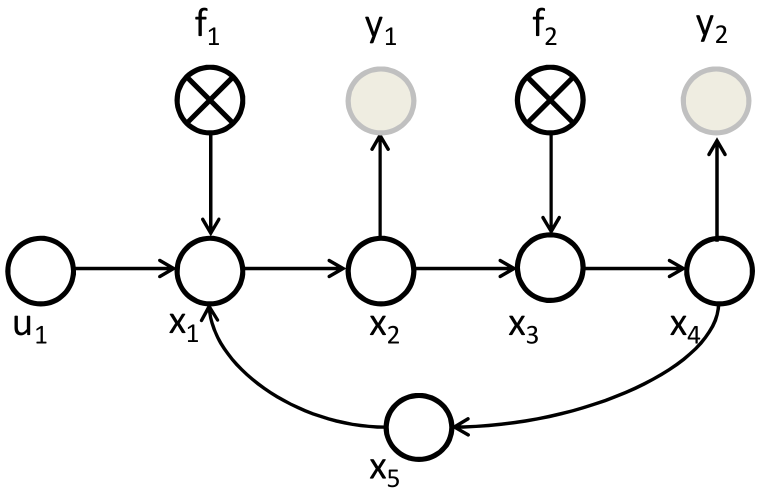
Figure 1presents an exemplary GP graph [37].

Two residuals utilising models are used for fault detection:

$$r_1=y_1-x_2\left(u\right),r_2=y_2-x_4\left(u\right).$$

These residuals are sensitive for both faults $f_1$and$f_2$. The occurrence of$f_1$fault causes the occurrence of $s_1$symptom and then$s_2$symptom,$f_2$fault will cause the reverse symptom forming order -$s_2$will emerge first and then$s_1$. Thus, we can note:

$$e{s}_{1,2}\left(f_1\right) =〈s_1,s_2〉,e{s}_{1,2}\left(f_2\right) =〈s_2,s_1〉.$$

The above example shows that when measurements are appropriately selected in feedback systems, it is possible to design residuals characterised by different symptoms forming order for the same faults.

Assuming the lack of knowledge of the internal form of residuals and the GP graph, expert knowledge can be also used to determine the sequence of symptoms formation. However, it is not usually possible to unequivocally define this sequence for all faults. Thus, the knowledge gained in this way is not complete. It is not possible in practice to experimentally obtain knowledge about the sequence of symptoms.

5. Inference about Faults with the Use of Incomplete Knowledge about the Sequence of Symptoms Forming

5.1. Assumptions

(a)

The relationship between the faults and diagnostic signals is known and takes the form of rule (12).

(b)

Some relationships between the times of symptom formation are known and have the form of elementary sequences $e{s}_{j,p}\left(f_k\right)=\langle s_j,s_p\rangle$. The set of these sequences is usually not complete.

(c)

As in many other works [40,41], we assume the occurrence of single faults.

(d)

We assume that the diagnostic signal is sensitive or not to a given fault. This means that the subset $V_{kj}$, if it contains zero, is a one-element set (it does not contain any other value of the diagnostic signal being a fault symptom).

5.2. Principle of Formulating the Diagnosis

Inference occurs after each symptom is observed. The first detected symptom initiates the fault isolation algorithm. Rules of the form (12) and known elementary sequences collected in the knowledge base are used to formulate a diagnosis. The diagnosis is formulated in steps after observing subsequent symptoms.

If the symptom $s_a=v_p\ne 0$ is observed, then the inference begins with the rule in which this premise occurs. The rule conclusion specifies a subset of faults which are the cause of the detected symptom $f\in F\left(s_a=v_p\right)$. The set $F\left(s_a=v_p\right)$ is the first diagnosis:

$$DG{N}_1^{*}=F(s_a=v_p).$$

(15)

This set can be reduced even before the next symptom is observed as a result of the analysis of elementary sequences containing the signal $s_a$. If for $f_l\in DG{N}_1^{*}$ there is elementary sequence $e{s}_{n,a}\left(f_l\right)=\langle s_n,s_a\rangle$, it means that fault $f_l$ activates symptom $s_n$ first, and then the symptom $s_a$. As the symptom $s_n$ did not occur, the fault $f_l$ should be eliminated from the set of faults indicated in the diagnosis:

$$DG{N}_1=DG{N}_1^{*}\backslash \left\{f_l\in DG{N}_1^{*}:\vee e{s}_{n,a}\left(f_l\right)=\langle s_n,s_a\rangle \right\}.$$

(16)

In each subsequent step of inference, two elements are used to reduce the set of possible faults:

• a subset of faults activating the observed symptom,
• elementary sequences for the considered faults, in terms of eliminating those faults for which the elementary sequences are inconsistent with the observed.

As a result of the analysis of subsequent symptoms, the diagnosis formulated in the previous step is refined. The product of the set of possible faults indicated in the diagnosis from the previous step $DG{N}_{n-1}$ and the set of faults that could have been the cause of the analysed symptom $F(s_e=v_r)$ is determined. Due to the assumption of single faults, the reduction is as follows:

$$DG{N}_n^{*}=DG{N}_{n-1}\cap F(s_e=v_r).$$

(17)

After each analysis of the content of the rule conclusion, the set of possible faults is reduced based on the analysis of elementary sequences stored in the knowledge base.

The sequences for $f_k\in DG{N}_n^{*}$ faults are analysed. For a given fault $f_l\in DG{N}_n^{*}$ we check if there is a signal $s_j$, the symptom of which should appear earlier than the observed symptom $s_e=v_r\ne 0$. The corresponding elementary sequence is: $e{s}_{j,e}\left(f_l\right) =\langle s_j,s_e\rangle$. If there is such a sequence in the knowledge base, we infer that $f_l$ fault did not occur. Its symptom $s_j\ne 0$ would occur earlier than the symptom $s_e=v_r\ne 0$. Such a fault is eliminated from the set of possible faults. This procedure is repeated for all $f_k\in DG{N}_n^{*}$ faults. The new, more accurate diagnosis takes the form of:

$$DG{N}_n=DG{N}_n^{*}\backslash \left\{f_l\in DG{N}_n^{*}:\vee e{s}_{j,e}\left(f_l\right) =\langle s_j,s_e\rangle \right\}.$$

(18)

The current diagnosis $DG{N}_n$ is available at any time of inference. It indicates the subset of possible faults that includes the existing fault. It is the upper limit of the set of possible faults.

The improvement of the fault isolation algorithm in complex systems is the limitation of the set of diagnostic signals used in a given inference process. This set can be determined after the first symptom is observed, according to the formula:

$$S_0=\{s_j\in S:DG{N}_1^{*}\cap F(s_j)\ne \varnothing \}\backslash s_a; S_0\subset S.$$

(19)

6. An Example, a Comparison with Other Methods

6.1. A Diagnosed Object

The usability of the proposed method will be analysed in an example of diagnostics of serially connected liquid storage tanks (Figure 2). The systems of connected in series tanks [10] are typical objects used to present diagnostic methods of dynamic processes due to the ease of understanding the principles of their operation and a significant degree of complication resulting from existing feedback in the diagnosed process itself.

The flow between two tanks is specified by the following equation:

$$F_i={\alpha }_i{S}_i\sqrt{2\mathrm{g}\left(L_{i-1}-L_i\right)}$$

(20)

where: ${\alpha }_i$—flow coefficient, $S_i$—flow section, and $g$—acceleration of gravity.

The change of the volume in the tank is described by the dependence:

$$A\frac{d{L}_i}{dt}=F_i-{\mathrm{F}}_{i+1}$$

(21)

where $A_i$ is the cross-sectional area of the tank.

The cause-and-effect graph of the process is presented in Figure 3.

6.2. Elements of the Diagnostic System

Diagnostics of the object is conducted on the basis of three available pressure measurements: flow $F_1$ and levels $L_1$ and $L_4$. Attainable partial models of the following structures were used: $L_1=f_1\left(F_1\right)$, $L_4=f_2\left(F_1\right)$ and $L_4=f_3\left(L_1\right)$. Application of models created on the basis of experimental data (neural, fuzzy) was assumed. The corresponding residuals are:

$$r_1=L_1-{\mathsf{\Phi }}_1\left(F_1\right),$$

(22)

$$r_2=L_4-{\mathsf{\Phi }}_2\left(F_1\right),$$

(23)

$$r_3=L_4-{\mathsf{\Phi }}_3\left(L_1\right).$$

(24)

The list of faults (

Table 2. Set of faults.

Fault Symbol	Description
$f_1$	leak in tank 1
$f_2$	leak in tank 2
$f_3$	leak in tank 3
$f_4$	leak in tank 4
$f_5$	clogging in the pipe between tanks 1 and 2
$f_6$	clogging in the pipe between tanks 2 and 3
$f_7$	clogging in the pipe between tanks 3 and 4
$f_8$	fault of $F_1$ measuring path
$f_9$	fault of $L_1$ measuring path
$f_{10}$	fault of $L_4$ measuring path

) covers leaks in the tanks, clogging of the channels connecting the tanks, and faults of the measuring paths.

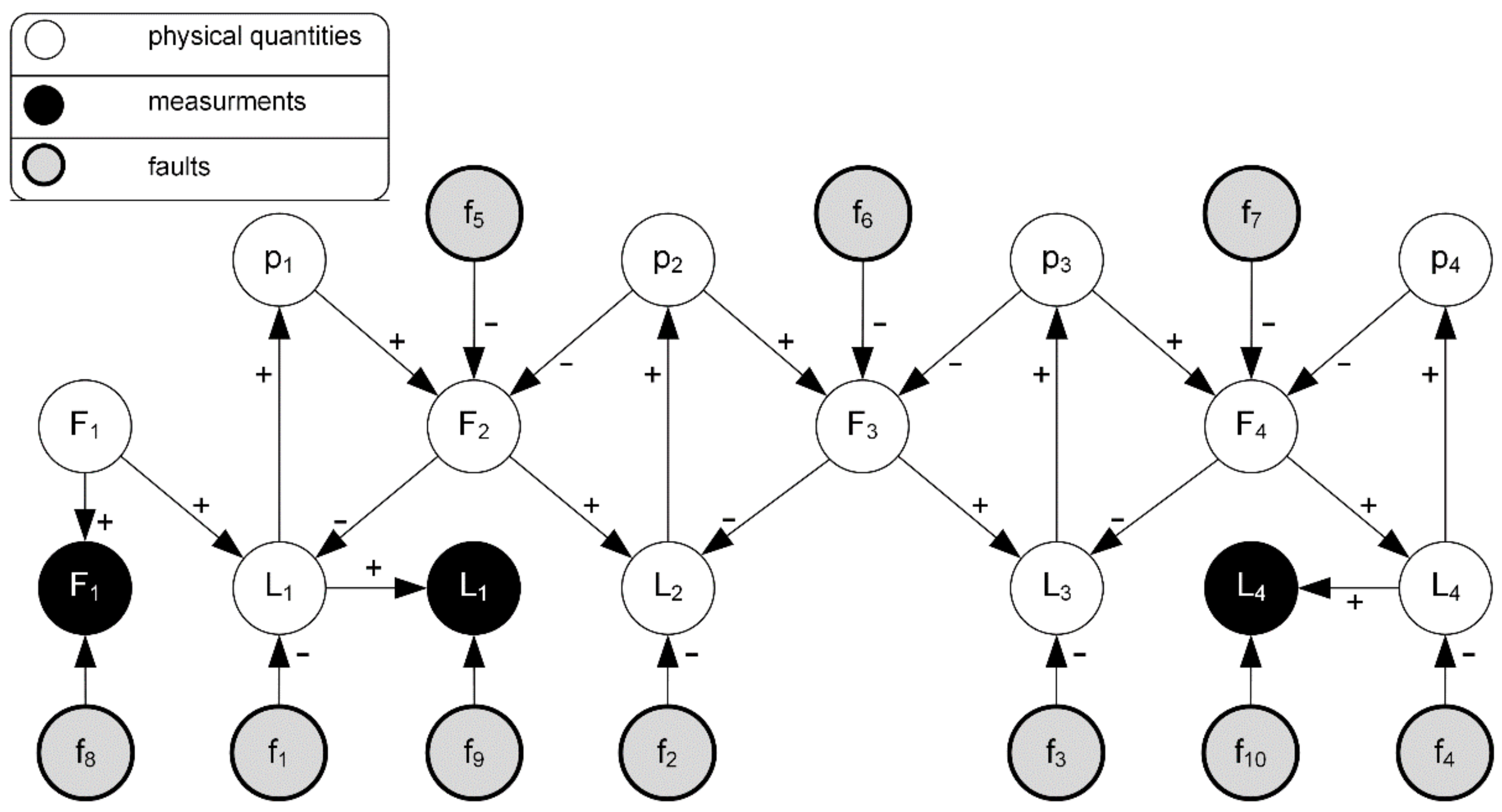
Figure 4 presents a GP graph of a process for a set of liquid storage tanks acknowledging the influence of the faults on the process variables. The sensitivity of the particular residuals for the faults may be determined on the basis of expert knowledge or read from a GP graph:

$$r_1=r_1\left(f_1,f_2,f_3,f_4,f_5,f_6,f_7,f_8,f_9\right),$$

(25)

$$r_2=r_2\left(f_1,f_2,f_3,f_4,f_5,f_6,f_7,f_8,f_{10}\right),$$

(26)

$$r_3=r_3\left(f_2,f_3,f_4,f_6,f_7,f_9,f_{10}\right),$$

(27)

Note that the measurement of the input signal to the models cuts the sensitivity of the residual using this model from the faults influencing the measured variable. Therefore, residuum $r_3$ is not sensitive to a fault $f_1$.

The Fault Isolation System—FIS for the set of serially connected liquid storage tanks developed assuming trivalent evaluation of the residuals is presented in

Table 3. FIS—Fault Isolation System.

	${\mathit{f}}_1$	${\mathit{f}}_2$	${\mathit{f}}_3$	${\mathit{f}}_4$	${\mathit{f}}_5$	${\mathit{f}}_6$	${\mathit{f}}_7$	${\mathit{f}}_8$	${\mathit{f}}_9$	${\mathit{f}}_{10}$	Evaluation Threshold/ΔOFF
${\mathit{s}}_1$	−1	−1	−1	−1	+1	+1	+1	−1,+1	−1,+1		0.0031/−20%
${\mathit{s}}_2$	−1	−1	−1	−1	−1	−1	−1	−1,+1		−1,+1	0.0018/−20%
${\mathit{s}}_3$		−1	−1	−1	−1	−1	−1		−1,+1	−1,+1	0.0019/−20%

.

In Table 3, the subsets of possible values of diagnostic signals are given for the faults of measuring paths $f_8$, $f_9$ and $f_{10}$. Not all combinations of values may occur. In

Table 4. Physically possible three-valued fault signatures.

	${\mathit{f}}_1$	${\mathit{f}}_2$	${\mathit{f}}_3$	${\mathit{f}}_4$	${\mathit{f}}_5$	${\mathit{f}}_6$	${\mathit{f}}_7$	${\mathit{f}}_8$		${\mathit{f}}_9$		${\mathit{f}}_{10}$
								-	+	-	+	-	+
${\mathit{s}}_1$	−1	−1	−1	−1	+1	+1	+1	+1	−1	−1	+1
${\mathit{s}}_2$	−1	−1	−1	−1	−1	−1	−1	+1	−1			−1	+1
${\mathit{s}}_3$		−1	−1	−1	−1	−1	−1			+1	−1	−1	+1

, the physically possible three-valued fault signatures are given.

It should be noted that residual $r_2$ responds with an impulse to the appearance of clogging in the pipe connecting the tanks (faults $f_5$, $f_6$, $f_7$). The value in the transient state after fault appearance deviates from zero, and after the levels in the tanks rises, it gradually tends to zero, to a steady-state.

Analysing the symptoms forming order (under the assumption of the same geometric parameters of tanks and connecting the pipelines) on the basis of a GP graph (Figure 4), one may define the elementary sequences listed in

Table 5. Elementary sequences for the diagnosed process.

${\mathit{f}}_{\mathit{k}}$	Elementary Sequences
$f_1$	$e{s}_{1,2}\left(f_1\right) =\langle s_1,s_2\rangle$
$f_2$	$e{s}_{1,2}\left(f_2\right) =\langle s_1,s_2\rangle$$, e{s}_{1,3}\left(f_2\right) =\langle s_1,s_3\rangle$,
$f_3$	$e{s}_{1,2}\left(f_3\right) =\langle s_2,s_1\rangle$$, e{s}_{1,3}\left(f_3\right) =\langle s_3,s_1\rangle$,
$f_4$	$e{s}_{1,2}\left(f_4\right) =\langle s_2,s_1\rangle$$, e{s}_{1,3}\left(f_4\right) =\langle s_3,s_1\rangle$
$f_5$	$e{s}_{1,2}\left(f_5\right) =\langle s_1,s_2\rangle$$, e{s}_{1,3}\left(f_5\right) =\langle s_1,s_3\rangle$
$f_6$	lack
$f_7$	$e{s}_{1,2}\left(f_7\right) =\langle s_2,s_1\rangle$$, e{s}_{1,3}\left(f_7\right) =\langle s_3,s_1\rangle$,

.

The sensor fault effects on the residuals are immediate. Therefore, the sequences for these faults have not been determined.

Table 6. List of pairs of elementary sequences distinguishing faults.

$e{s}_{1,2}\left(f_1\right) =\langle s_1,s_2\rangle$$, e{s}_{1,2}\left(f_3\right) =\langle s_2,s_1\rangle$	$e{s}_{1,2}\left(f_1\right) =\langle s_1,s_2\rangle$$, e{s}_{1,2}\left(f_4\right) =\langle s_2,s_1\rangle$
$e{s}_{1,2}\left(f_1\right) =\langle s_1,s_2\rangle$$, e{s}_{1,2}\left(f_7\right) =\langle s_2,s_1\rangle$
$e{s}_{1,2}\left(f_2\right) =\langle s_1,s_2\rangle$$, e{s}_{1,2}\left(f_3\right) =\langle s_2,s_1\rangle$	$e{s}_{1,3}\left(f_2\right) =\langle s_1,s_3\rangle$$, e{s}_{1,3}\left(f_3\right) =\langle s_3,s_1\rangle$
$e{s}_{1,2}\left(f_2\right) =\langle s_1,s_2\rangle$$, e{s}_{1,2}\left(f_4\right) =\langle s_2,s_1\rangle$	$e{s}_{1,3}\left(f_2\right) =\langle s_1,s_3\rangle$$, e{s}_{1,3}\left(f_4\right) =\langle s_3,s_1\rangle$
$e{s}_{1,2}\left(f_2\right) =\langle s_1,s_2\rangle , e{s}_{1,2}\left(f_7\right) =\langle s_2,s_1\rangle$	$e{s}_{1,3}\left(f_2\right) =\langle s_1,s_3\rangle$$, e{s}_{1,3}\left(f_7\right) =\langle s_3,s_1\rangle$
$e{s}_{1,2}\left(f_3\right) =\langle s_2,s_1\rangle$$, e{s}_{1,2}\left(f_5\right) =\langle s_2,s_1\rangle$	$e{s}_{1,3}\left(f_3\right) =\langle s_3,s_1\rangle$$, e{s}_{1,2}\left(f_5\right) =\langle s_1,s_3\rangle$
$e{s}_{1,2}\left(f_4\right) =\langle s_2,s_1\rangle$$, e{s}_{1,2}\left(f_5\right) =\langle s_1,s_2\rangle$	$e{s}_{1,3}\left(f_4\right) =\langle s_3,s_1\rangle$$, e{s}_{1,2}\left(f_5\right) =\langle s_1,s_3\rangle$
$e{s}_{1,2}\left(f_5\right) =\langle s_1,s_2\rangle$$, e{s}_{1,2}\left(f_7\right) =\langle s_2,s_1\rangle$	$e{s}_{1,3}\left(f_5\right) =\langle s_1,s_3\rangle$$, e{s}_{1,3}\left(f_7\right) =\langle s_3,s_1\rangle$

lists the pairs of elementary sequences that distinguish faults.

Note that the elementary sequences ensure distinguishability, amongst others, of pairs of faults: $f_2$ and $f_4$, $f_2$ and $f_7$, $f_3$ and $f_5$, $f_5$ and $f_7$, which are not distinguishable on the basis of binary signatures, and pairs $f_2$ and $f_3$, $f_3$ and $f_4$, $f_3$ and $f_5$ indistinguishable on the basis of three-valued signatures. For example,

Table 7. Alternative signatures for $f_2$ and $f_3$ faults containing the values of diagnostic signals and the sequence of symptoms.

	${\mathit{f}}_2$		${\mathit{f}}_3$
1	$s_1=-1$	$s_1=-1$	$s_2=-1$	$s_3=-1$
2	$s_2=-1$	$s_3=-1$	$s_3=-1$	$s_2=-1$
3	$s_3=-1$	$s_2=-1$	$s_1=-1$	$s_1=-1$

lists alternative signatures considering the values and sequence of symptoms for $f_2$ and $f_3$ faults. All of them make it possible to distinguish these faults, which are indistinguishable based on binary and three-valued signatures.

It should be noted that not only elementary sequences creating pairs unconditionally distinguishing listed in Table 6 are useful to distinguish between faults. The others can also be useful in cases of conditional distinguishability on the basis of elementary sequences, according to Definition 3.

6.3. Examples of Inference Based on the Proposed Algorithm

Two examples of the course of diagnosis according to the proposed algorithm are presented below.

Simulation 1.

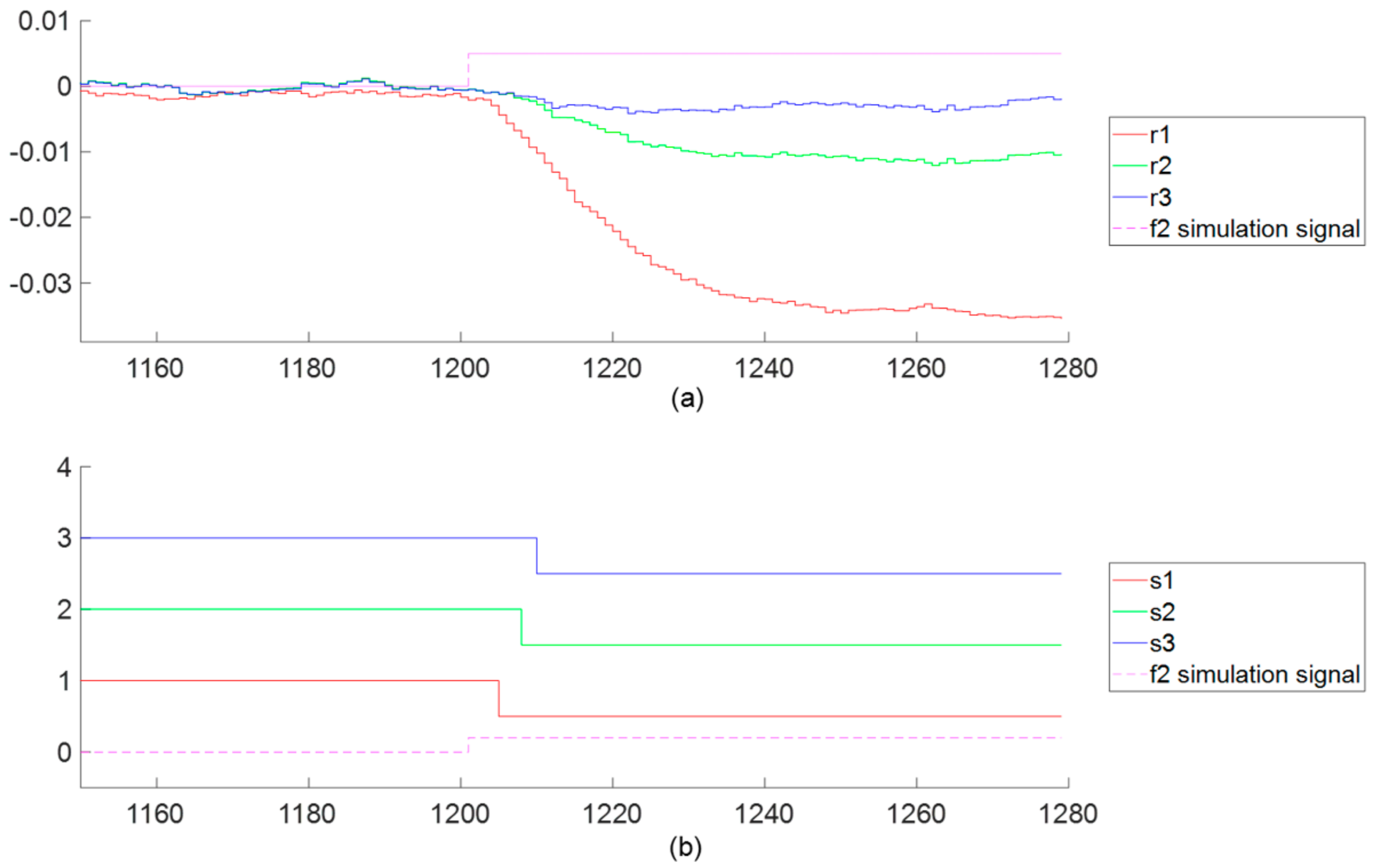
This simulation illustrates the case where all three residuals deviate from zero due to the introduction of fault$f_2$. Figure 5shows the recorded time series of the residuals and diagnostic signals.

• The first observed symptom:$s_1=-1$. The first generated diagnosis is as follows: $(s_1=-1)\Rightarrow DG{N}_1^{*}=\left\{f_1,f_2,f_3,f_4,f_8,f_9\right\}$. A set of tests useful for the fault diagnosis: $S_0=\left\{s_1,s_3\right\}$. The following elementary sequences:$e{s}_{1,3}\left(f_3\right) =\langle s_2,s_1\rangle$,$e{s}_{1,2}\left(f_4\right) =\langle s_2,s_1\rangle$,$e{s}_{1,3}\left(f_4\right) =\langle s_3,s_1\rangle$eliminate the possibility of faults$f_3$and$f_4$, because the first symptom was$s_1=-1$. Thus, the reduced diagnosis takes the form of:$DG{N}_1=\left\{f_1,f_2,f_8,f_9\right\}$.
• The next symptom:$s_2=-1$indicates faults in a subset:$F\left(s_2=-1\right)=\left\{f_1,f_2,f_3,f_4,f_5,f_6,f_7,f_8,f_{10}\right\}$. Thus:$DG{N}_2^{*}=DG{N}_1\cap \{F(s_2=-1)\}=\left\{f_1,f_2,f_8\right\}$and$DG{N}_2=DG{N}_2^{*}$.
• The last observer symptom:$s_3=-1$,$F\left(s_3=-1\right)=\{f_2,f_3,f_4,f_5,f_6,f_7,f_9,f_{10}\}$enables the formulation of the final diagnosis:$DG{N}_3^{*}=DG{N}_2\cap \{F(s_4=-1)\}=\left\{f_2\right\}$. $DG{N}_3=DG{N}_3^{*}=\left\{f_2\right\}$.

In the case of reasoning on the basis of signatures (without taking into account the information about the order of symptoms) in the transitional state $\langle s_1=-1,{ s}_2=-1,s_3=0\rangle$ a temporary false diagnosis appears, indicating faults $f_1$ or $f_8$. In this case, the final diagnosis shows three indistinguishable faults $f_2$, $f_3$ and $f_4$.

Simulation 2.

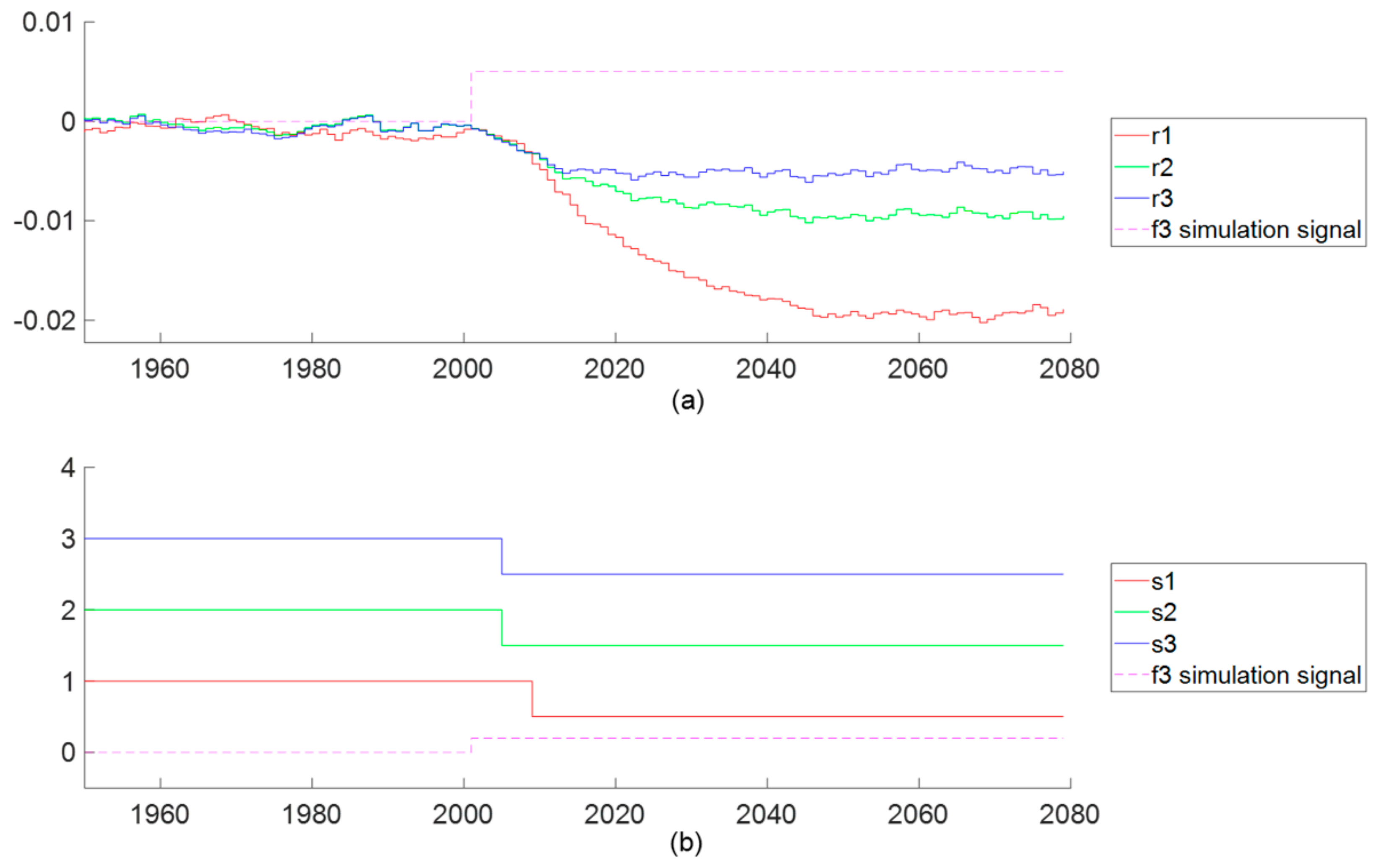
In the second experiment also all three residuals deviate from zero due to the introduction of fault$f_3$. Figure 6shows the recorded time series of the residuals and diagnostic signals. The values of diagnostic signals in a steady-state are the same as in Simulation 1, but the order of the symptoms is different.

In the second scenario fault$f_3$is simulated. The inference is carried out according to analogous steps:

• The first observed symptom:$s_3=-1$. The first generated diagnosis:$(s_3=-1)\Rightarrow DG{N}_1^{*} =\left\{f_2,f_3,f_4,f_5,f_6,f_7,f_9,f_{10}\right\}$. A set of tests useful for the fault diagnosis:$S_0=\left\{s_1,s_2\right\}$. The following elementary sequences:$e{s}_{1,3}\left(f_2\right) =〈s_1,s_3〉$,$e{s}_{1,2}\left(f_5\right) =〈s_1,s_3〉$eliminate faults$f_2$and$f_5$. The reduced diagnosis:$DG{N}_1 =\left\{f_3,f_4,f_6,f_7,f_9,f_{10}\right\}$.
• The next symptom:$s_2=-1$indicates faults in a subset:$F\left(s_2=-1\right)=\left\{f_1,f_2,f_3,f_4,f_8,f_{10}\right\}$. Thus:$DG{N}_2^{*}=DG{N}_1\cap \{F(s_2=-1)\}=\left\{f_3,f_4,f_{10}\right\}$and$DG{N}_2=DG{N}_2^{*}$.
• The last observer symptom:$s_1=-1$,$F\left(s_1=-1\right)=\{f_1,f_2,f_3,f_4,f_8,f_9\}$enables the formulation of the final diagnosis:$DG{N}_3^{*}=DG{N}_2\cap \{F(s_1=-1)\}=\left\{f_3,f_4\right\}$. $DG{N}_3=DG{N}_3^{*}=\left\{f_3,f_4\right\}$.

In the case of reasoning based on the signatures, the final diagnosis shows three indistinguishable faults $f_2$, $f_3$, $f_4$. In the transition state $\langle s_1=0,{ s}_2=-1,s_3=-1\rangle$ there is a temporary false diagnosis indicating a fault $f_{10}$.

It should be noted that the fault $f_2$ is indistinguishable from $f_3$ on the basis of three-valued diagnostic signals. Symptom sequence analysis ensures isolability.

6.4. Results Comparison

To compare the diagnosis results with a new method called Tree-Valued Symptoms Sequence Fault Isolation (TVSSFI) with other known algorithms, it was assumed that all symptoms included in the signature of each failure would be observable after the appearance of the fault. Methods robust to symptom delays were considered for comparison:

• Row Reasoning—DX,
• Symptom Based Reasoning—SBR,
• Symptoms Sequence Fault Isolation—SSFI,
• Tree Value Row Reasoning—TVRR.
• the new method—Tree-Valued Symptoms Sequence Fault Isolation—TVSSFI.

The occurrence of single faults was assumed. Therefore, potential diagnoses concerning multiple faults generated by DX methods were not considered. Methods DX, SBR and SSFI, utilise binary residual evaluation, while methods TVRR and TVSSFI three values evaluation.

The first comparison concerns the theoretical maximum number of different diagnoses ${\mathrm{L}}_{\mathrm{MAX}}$ obtained by the analysed methods. It depends on the number of possible diagnostic signal values and the number of possible sequences. The general formula for ${\mathrm{L}}_{\mathrm{MAX}}$ when the sequences are considered is as follows:

$${\mathrm{L}}_{\mathrm{MAX}}={\mathrm{M}}^{\mathrm{J}}\mathrm{J}!,$$

(28)

where M is the number of diagnostic signal values and J is the number of diagnostic signals. The number of possible combinations of diagnostic signal values is ${\mathrm{M}}^{\mathrm{J}}$ and the number of possible sequences is $\mathrm{J}!$.

When the sequences are not considered, the formula (28) takes the form:

$${\mathrm{L}}_{\mathrm{MAX}}={\mathrm{M}}^{\mathrm{J}}.$$

(29)

The

Table 8. Summary of the theoretical value of the maximum number of diagnoses $L_{MAX}$ for the analysed methods.

Method	DX	SBR	SSFI	TVRR	TVSSFI
$L_{MAX}$$, \mathrm{J}=3$	8	8	48	27	156

shows the limited capabilities of the methods, but the actual values are much smaller due to the physical limitations in each diagnosed process. However, the summary illustrates the importance of using the symptom sequence in the process of diagnostic inference.

Table 9. List of diagnoses obtained by inference methods on the basis of BMD or FIS rows under the assumption of single faults.

${\mathit{f}}_{\mathit{k}}$	${\mathit{s}}_{\mathit{j}}$	DX/SBR	SSFI	TVRR	TVSSFI	${\mathit{s}}_{\mathit{j}}$
$f_1$	$1,1,0$	$f_1,f_2,f_3,f_4,f_5,f_6,f_7,f_8$	$f_1,f_2,f_5,f_6,f_8$	$f_1,f_2,f_3,f_4,f_8$	$f_1,f_2,f_8$	$-1,-1,0$
$f_2$	$1,1,1$	$f_2,f_3$$, f_4$$, f_5,f_6,f_7$	$f_2, f_5,f_6$	$f_2,f_3,f_4$	$f_2$	$-1,-1,-1$
$f_3$	$1,1,1,1$	$f_2,f_3,f_4, f_5,f_6,f_7$	$f_3,f_4,f_6,f_7$	$f_2,f_3,f_4$	$f_3,f_4$	$-1,-1,-1$
$f_4$	$1,1,1$	$f_2,f_3,f_4$$, f_5,f_6,f_7$	$f_3,f_4,f_6,f_7$	$f_2,f_3,f_4$	$f_3,f_4$	$-1,-1,-1$
$f_5$	$1,1/0,1$	$f_2,f_3,f_4,f_5,f_6,f_7$	$f_2,f_5,f_6$	$f_5,f_6,f_7$	$f_5,f_6$	$+1,-1/0,-1$
$f_6$	$1,1/0,1$	$f_2,f_3,f_4,f_5,f_6,f_7$	$f_3,f_4,f_6,f_7$ or $f_2,f_5,f_6$	$f_5,f_6,f_7$	$f_5,f_6$ or $f_6,f_7$	$+1,-1/0,-1$
$f_7$	$1,1/0,1$	$f_2,f_3,f_4,f_5,f_6,f_7$	$f_3,f_4,f_6,f_7$	$f_5,f_6,f_7$	$f_6,f_7$	$+1,-1/0,-1$
$f_8$	$1,1,0$	$f_1,f_2,f_3,f_4,f_5,f_6,f_7, f_8$	$f_1,f_2,f_5,f_6,f_8$ or $f_3,f_4,f_6,f_7,f_8$	$f_1,f_2,f_3,f_4,f_8$	$f_1,f_2,f_8$ or $f_3,f_4,f_8$	$-1,-1,0$
				$f_8$	$f_8$	$+1,+1,0$
$f_9$	$1,0,1$	$f_2,f_3,f_4,f_5,f_6,f_7,f_9$	$f_2,f_5,f_6,f_9$ or $f_3,f_4,f_6,f_7,f_9$	$f_9$	$f_9$	$-1,0,+1$
				$f_5,f_6,f_7,f_9$	$f_5,f_6,f_9$ or $f_6,f_7,f_9$	$+1,0,-1$
$f_{10}$	$0,1,1$	$f_2,f_3,f_4,f_5,f_6,f_7,f_{10}$	$f_2,f_3,f_4,f_5,f_6,f_7,f_{10}$	$f_2,f_3,f_4,f_5,f_6,f_7,f_{10}$	$f_2,f_5,f_6,f_{10}$ or $f_3,f_4,f_6,f_7,f_{10}$	$0,-$$1,-$1
				$f_{10}$	$f_{10}$	$0,+$$1,+$1

summarises the diagnoses obtained by various inference methods based on the BMD or FIS rows. All these methods prevent the generation of false diagnoses due to symptom delays.

On the basis of Table 9, it is possible to compare the distinguishability of faults in the case of the considered process and the analysed methods of diagnosis.

The accuracy of a single diagnosis is defined as the reciprocal of the number of faults $d_i$ indicated in the diagnosis. Thus, the accuracy of the fault $f_i$ isolation is the average value of the accuracy of diagnoses generated in the event of this fault. This accuracy can be determined from Table 9. The diagnosing accuracy index D is defined as the average diagnosis accuracy for all K faults:

$$D=\frac{1}{K}{{\displaystyle \sum }}_{i=1}^K\frac{1}{d_i}.$$

(30)

The diagnostic accuracy index $D$ was used as a measure of fault distinguishability.

Table 10. List of diagnostic accuracy indicators for the tested methods.

Method	DX	SBR	SSFI	TVRR	TVSSFI
$D$	0.154	0.154	0.247	0.400	0.577

presents the calculated values of the diagnostic accuracy index for the tested methods.

Table 10 illustrates the increase in the value of the diagnosis accuracy index using the three-valued residuals evaluation and the knowledge of elementary symptom sequences. The new inference method allows the determination of the highest fault distinguishability in the case of the analysed process among the methods resistant to symptom delays. This proves the effectiveness of the proposed algorithm.

7. Discussion and Conclusions

We present a new method of diagnostic inference. It is robust against the possibility of formulating false diagnoses due to different delays of symptoms of the same fault. In many cases, this method allows increasing the obtained fault distinguishability compared to other known methods. The results of the comparison for the exemplary case are given in Section 6.4. The method is based on three-valued residual evaluation, and it uses the knowledge of elementary sequences of symptoms of particular faults. Such knowledge can be obtained based on expert knowledge and the analysis of a cause-and-effect graph considering the impacts of faults. A significant advantage of the proposed approach is that this knowledge is not required to be complete, i.e., it is not necessary to define the sequence of all symptoms for all faults. Only those elementary sequences are used that are known. However, the increase in fault distinguishability is the more remarkable, the more complete the knowledge of the elementary sequences of symptoms is.

Known approaches to fault isolation robust against the possibility of formulating false diagnoses due to different delays of symptoms were based on the inference with the binary evaluation of residuals. In most cases, they did not make use of the knowledge regarding the sequence of symptoms. This resulted in a low distinguishability of faults.

On the other hand, the diagnostic methods using the internal form of the residuals are not valuable for the diagnostics of industrial processes due to the difficulties and high costs of obtaining models considering the influence of faults.

The presented method is advantageous in industrial installations poorly equipped with instruments for which the fault distinguishability obtained based only on the values of diagnostic signals is low. In these cases, the use of additional knowledge about the order of symptoms defined in the form of elementary sequences allows for a significant increase in distinguishability of faults (even over 40% concerning the BS and DX methods, as shown in the analysed example).

The method was developed under the assumption of single faults. This assumption only apparently limits the scope of the method’s application. In the vast majority of methods, the inference begins with the search for single faults, which emergence in a short period is much more likely than the emergence of multiple faults. At this stage of diagnosis, the presented method can be successfully applied. The lack of a solution (diagnosis) in the single fault class results in a double fault class solution search. At this stage, known inference methods for multiple faults are used. So far, there are no known methods of distinguishing multiple faults using the knowledge of the sequences of symptoms. It is a topic of future research.

References

1. Blanke, M.; Kinnaert, M.; Lunze, J.; Staroswiecki, M. Diagnosis and Fault-Tolerant Control; Springer: New York, NY, USA, 2015. [Google Scholar]
2. Chen, J.; Patton, R. Robust Model Based Fault Diagnosis for Dynamic Systems; Kluwer Akademic Publishers: Boston, MA, USA, 1999. [Google Scholar]
3. Gertler, J. Fault Detection and Diagnosis in Engineering Systems; Marcel Dekker, Inc.: New York, NY, USA; Basel, Switzerland; Hong Kong, China, 1998. [Google Scholar]
4. Isermann, R. Fault Diagnosis Systems. An Introduction from Fault Detection to Fault Tolerance; Springer: Berlin/Heidelberg, Germany, 2006. [Google Scholar] [CrossRef]
5. Korbicz, J.; Kościelny, J.M.; Kowalczuk, Z.; Cholewa, W. Fault Diagnosis: Models, Artificial Intelligence Methods, Applications, 1st ed.; Springer: Berlin, Germany; New York, NY, USA, 2004. [Google Scholar] [CrossRef] [Green Version]
6. Patton, R.; Frank, P.; Clark, R. (Eds.) Issues of Fault Diagnosis for Dynamic Systems; Springer: Berlin/Heidelberg, Germany, 2000. [Google Scholar]
7. Witczak, M. Modelling and Estimation Strategies for Fault Diagnosis of Non-Linear Systems. From Analytical to Soft Computing Approaches; Springer: Berlin, Germany, 2007. [Google Scholar] [CrossRef]
8. Kościelny, J.M.; Syfert, M. Application properties of methods for fault detection and isolation in the diagnosis of complex large-scale processes. Bull. Pol. Acad. Sci. Tech. Sci. 2014, 62, 571–582. [Google Scholar] [CrossRef]
9. Combastel, C.; Gentil, S.; Rognon, J.P. Toward a Better Integration of Residual Generation and Diagnostic Decision. IFAC Proc. Vol. 2003, 36, 69–74. [Google Scholar] [CrossRef]
10. Daigle, M.; Koutsoukos, X.; Biswas, G. Relative Measurement Orderings in Diagnosis of Distributed Physical Systems. In Proceedings of the 43rd Annual Allerton Conference on Communication, Control, and Computing, Monticello, IL, USA, 28–30 September 2005; pp. 1707–1716. [Google Scholar]
11. Kościelny, J.M. Fault Isolation in Industrial Processes by Dynamic Table of States Method. Automatica 1995, 31, 747–753. [Google Scholar] [CrossRef]
12. Kościelny, J.M.; Syfert, M. The issue of symptom based diagnostic reasoning. In Recent Advances in Mechatronics; Jabłoński, R., Turkowski, M., Szewczyk, R., Eds.; Springer: Berlin/Heidelberg, Germany, 2007; pp. 167–171. [Google Scholar]
13. Meseguer, J.; Puig, V.; Escobet, T. Fault Diagnosis using a Timed Descrete Event Approach based on interval Observers. IFAC Proc. Vol. 2008, 41, 6914–6919. [Google Scholar] [CrossRef]
14. Puig, V.; Schmid, F.; Quevedo, J.; Pulido, B. A New Fault Diagnosis Algorithm that Improves the Integration of Fault Detection and Isolation. In Proceedings of the 44th IEEE Conference on: Decision and Control, Seville, Spain, 15 December 2005; pp. 3809–3814. [Google Scholar]
15. Syfert, M.; Kościelny, J.M. Diagnostic Reasoning Based on Symptom Forming Sequence. IFAC Proc. Vol. 2009, 42, 89–94. [Google Scholar] [CrossRef]
16. Gertler, J. Analitical redunduncy methods in fault detection and isolation-Survey and Synthesis. IFAC Proc. Vol. 1991, 24, 9–21. [Google Scholar] [CrossRef]
17. Cordier, M.-O.; Dague, P.; Lévy, F.; Montmain, J.; Staroswiecki, M.; Travé-Massuyès, L. Conflicts versus analytical redundancy relations: A comparative analysis of the model based diagnosis approach from the artificial intelligence and automatic control perspectives. IEEE Trans. Syst. Man Cybern. Part B 2004, 34, 2163–2177. [Google Scholar] [CrossRef] [PubMed]
18. Travé-Massuyès, L. Bridges between diagnosis theories from control and AI perspectives. In Intelligent Systems in Technical and Medical Diagnostics; Korbicz, J., Kowal, M., Eds.; Series: Advances in Intelligent Systems and Computing; Springer: Berlin/Heidelberg, Germany, 2014; Volume 230, pp. 3–28. [Google Scholar]
19. Reiter, R.A. Theory of Diagnosis from First Principles. Artif. Intell. 1987, 32, 57–95. [Google Scholar] [CrossRef]
20. Frank, P.M. Fault diagnosis in dynamic systems using analytical and knowledge-based redundancy. Automatica 1990, 26, 459–474. [Google Scholar] [CrossRef]
21. Kościelny, J.M.; Bartyś, M.; Rzepiejewski, P.; Sá da Costa, J. Actuator fault distinguishability study for the DAMADICS benchmark problem. Control Eng. Pract. 2006, 14, 645–652. [Google Scholar] [CrossRef]
22. Lin, Z.; Duan, D.; Yang, Q.; Hong, X.; Cheng, X.; Yang, L.; Cui, S. Data-Driven Fault Localization in Distribution Systems with Distributed Energy Resources. Energies 2020, 13, 275. [Google Scholar] [CrossRef] [Green Version]
23. Calado, J.M.F.; Korbicz, J.; Patan, K.; Patton, R.J.; Sá da Costa, J.M.G. Soft computing approaches to fault diagnosis for dynamic systems. Eur. J. Control 2001, 7, 248–286. [Google Scholar] [CrossRef]
24. Nozari, H.A.; Nazeri, S.; Banadaki, H.D.; Castaldi, P. Model-free fault detection and isolation of a benchmark process control system based on multiple classifiers techniques—A comparative study. Control Eng. Pract. 2018, 73, 134–148. [Google Scholar] [CrossRef]
25. Jung, D.; Yew Ng, K.; Frisk, E.; Krysander, M. Combining model-based diagnosis and data-driven anomaly classifiers for fault isolation. Control Eng. Pract. 2018, 80, 146–156. [Google Scholar] [CrossRef]
26. Straka, O.; Punčochář, I. Decentralized and distributed active fault diagnosis: Multiple model estimation algorithms. Int. J. Appl. Math. Comput. Sci. 2020, 30, 239–249. [Google Scholar] [CrossRef]
27. Zhang, Z.; He, X. Fault-Structure-Based Active Fault Diagnosis: A Geometric Observer Approach. Energies 2020, 13, 4475. [Google Scholar] [CrossRef]
28. Kościelny, J.M.; Syfert, M.; Tabor, Ł. Application of Knowledge about Residuals Dynamics for Fault Isolation and Identification. In Proceedings of the Conference on Control and Fault-Tolerant Systems SysTol’13, Nice, France, 9–11 October 2013; pp. 275–280. [Google Scholar]
29. Shiozaki, J.; Shibata, B.; Matsuyama, H.; O’shima, E. Fault diagnosis of chemical processes sutilising signed directed graphs-improvement by using temporal information. In Proceedings of the IEEE International Workshop on Artificial Intelligence for Industrial Applications AI ’88, Hitachi City, Japan, 25–27 May 1988; pp. 461–466. [Google Scholar] [CrossRef]
30. Yang, F.; Xiao, D. Sensor location problem for large-scale complex systems in the framework of the dynamic Signed Directed Graph. In Proceedings of the IEEE International Conference on Systems, Man and Cybernetics ISIC, Montreal, QC, Canada, 7–10 October 2007; pp. 2843–2847. [Google Scholar] [CrossRef]
31. Bregon, A.; Alonso-González, C.J.; Pulido, B. Integration of simulation and state observers for online fault detection of nonlinear continuous systems. IEEE Trans. Syst. Man Cybern. Syst. 2014, 44, 1553–1568. [Google Scholar] [CrossRef]
32. Bregon, A.; Biswas, G.; Pulido, B. A Decomposition Method for Nonlinear Parameter Estimation in TRANSCEND. IEEE Trans. Syst. Man Cybern. Part A Syst. Hum. 2012, 42, 751–763. [Google Scholar] [CrossRef]
33. Bregon, A.; Pulido, B.; Biswas, G.; Koutsoukos, X.D. Generating Possible Conflicts From Bond Graphs Using Temporal Causal Graphs. In ECMS 2009 Proceedings; Otamendi, J., Bargiela, A., Luis Montes, J., Doncel Pedrera, L.M., Eds.; ECMS Press: Nashville, TN, USA, 2009; pp. 675–682. ISBN 978-0-9553018-8-9. [Google Scholar] [CrossRef]
34. Mosterman, P.J.; Biswas, G. Diagnosis of continuous valued systems in transient operating regions. IEEE Trans. Syst. Man Cybern. Part A Syst. Hum. 1999, 29, 554–565. [Google Scholar] [CrossRef] [Green Version]
35. Daigle, M.; Bregon, A.; Koutsoukos, X.; Biswas, G.; Pulido, B. A qualitative event-based approach to multiple fault diagnosis in continuous systems using structural model decomposition. Eng. Appl. Artif. Intell. 2016, 53, 190–206. [Google Scholar] [CrossRef]
36. Meseguer, J.; Puig, V.; Escobet, T. Fault diagnosis using a timed discrete-event approach based on interval observers: Application to sewer networks. IEEE Trans. Syst. Man Cybern. Part A Syst. Hum. 2010, 40, 900–916. [Google Scholar] [CrossRef]
37. Kościelny, J.M.; Syfert, M.; Rostek, K.; Sztyber, A. Fault isolability with different forms of the faults–symptoms relation. Int. J. Appl. Math. Comput. Sci. 2016, 26, 815–826. [Google Scholar] [CrossRef] [Green Version]
38. Kościelny, J.M.; Bartyś, M.; Rostek, K. The comparison of fault distinguishability approaches—Case study. Bull. Pol. Acad. Sci. Tech. Sci. 2019, 67, 1059–1068. [Google Scholar] [CrossRef]
39. Sztyber, A.; Ostasz, A.; Kościelny, J.M. Graph of a Process—A new tool for finding model’s structures in model based diagnosis. IEEE Trans. Syst. Man Cybern. Syst. 2015, 45, 1004–1017. [Google Scholar] [CrossRef]
40. Jung, D.; Khorasgani, H.; Frisk, E.; Krysander, M.; Biswas, G. Analysis of fault isolation assumptions when comparing model-based design approaches of diagnosis systems. IFAC-PapersOnLine 2015, 48, 1289–1296. [Google Scholar] [CrossRef]
41. Chanthery, E.; Travé-Massuyès, L.; Indra, S. Fault Isolation on Request Based on Decentralized Residual Generation. IEEE Trans. Syst. Man Cybern. Part A Syst. Hum. Institute Electr. Electron. Eng. 2015, 46, 598–610. [Google Scholar] [CrossRef]
Figure 1. Exemplary GP graph. Notation: u—inputs, y—control signals, f—faults, x—process variables (state variables).
Energies 14 02476 g001
Figure 2. Diagnosed process—set of serially connected pressure liquid storage tanks.
Energies 14 02476 g002
Figure 3. GP cause-and-effect graph of a process ( p i denotes pressure on the bottom of the i-th tank) including the mutual influence of process variables.
Energies 14 02476 g003
Figure 4. GP graph of the process, including fault influence on process variables.
Energies 14 02476 g004
Figure 5. Examples of diagnosing in case of f 2 fault: (a) residual values and simulated fault indicator; (b) diagnostic signal values (scaled to 0.5 ,   0.5 and shifted to s j number).
Energies 14 02476 g005
Figure 6. Examples of diagnosing in case of f 3 fault: (a) residual values and simulated fault indicator; (b) diagnostic signal values (scaled to 0.5 ,   0.5 and shifted to s j number).
Energies 14 02476 g006