Application of Identification Reference Nets for the Preliminary Modeling on the Example of Electrical Machines

Abstract

This paper presents the use of identification reference nets (IRNs) for modeling electric power system (EPS) components using electrical machines (EMs) as an example. To perform this type of task, a database of reference nets is necessary, to which the identification net (IN) of the modeled machine is adjusted. Both the IRN and IN are obtained by using a special algorithm that allows the relevant transfer function (TF) to be converted to the rounded trajectory. This type of modeling can be a useful tool for the initial determination of parameters included in the TF associated with the EM, preceding advanced parametric identification procedures, e.g., those based on artificial intelligence methods. Two types of electrical machines are considered, i.e., the squirrel-cage asynchronous (SCA) and brushless direct-current (BLDC) machines. The solution proposed in this paper is a new approach intended for modeling EPS components.

1. Introduction

Electrical machines (EMs) can be classified as one of the most important components of a power system [1]. For the proper design, diagnosis, use and control of the EMs, many modeling algorithms have been developed, from classical [2,3] to more advanced ones, which are currently based on artificial intelligence methods [4,5,6]. At the EM design stage, the model is dedicated to optimizing both its structure and parameters [7,8]. In terms of diagnosis, the model is the basis for synthesizing the appropriate state examination algorithm [9,10,11], while in the case of their use and control, the model is necessary for making the right decisions related to relevant exploiting activities [12,13]. It is noteworthy that the classical modeling methods are burdened with significant implementation costs [14], which very often prevents the implementation of new control techniques for the electric power system (EPS).

The equations defining the EMs are usually presented in a rectangular coordinate system, making it possible to determine the relationships between the relevant component of the space vectors of current or voltage and flux [15]. Hence, the modeling methods for the EMs are based on the measurement of peak-to-peak current with the pulsed voltage supply [16,17], measurement of steady-state characteristics [18,19], measurement of currents and voltages at constant velocity or determination of relevant time characteristics [20,21]. The EMs are most often used in the conditions of constantly changing parameters of the supply voltage (e.g., amplitude and frequency) and load torque [14]. Such conditions, in turn, influence the winding resistance, power losses and the relationship between the characteristics and, for example, the position and speed of the rotor [22]. As a result, there are constant changes in the transfer function (TF) parameters that represent the mathematical model of the EM, often to a significant extent [23].

Considering the above aspects, this paper proposes an application of the identification reference net (IRN) for the preliminary modeling of the EPS components using the EMs as an example. The IRN is a transformation of the step response which define the dynamic properties of the system under consideration. This response is obtained when the test excitation is performed in the form of a specific physical quantity (e.g., voltage, current, etc.). The IRN is an accessible tool to compare or match the mathematical models of different EPS components, e.g., electrical machines. This can be implemented by using selected numerical tools, ranging from the mean-square error criterion to the artificial intelligence, e.g., neural networks.

The aim of this preliminary modeling is to narrow down intervals for the parameters when using advanced methods for the parametric identification of the EPS [4,5,6]. Two types of EMs are considered, i.e., the squirrel-cage asynchronous (SCA) [24] and brushless direct-current (BLDC) [25] machines, which are currently widely used in the field of EPSs. The first one is most often used due to its high reliability, low cost, resistance to mechanical forces and infrequent maintenance requirements [26]. Compared with induction machines, the second type of EM is characterized by higher efficiency, greater power per mass unit, high overload torque and good control parameters [27].

The modeling with the use of IRN requires, first of all, determining the TF for the considered EPS component and then computing the corresponding step response [28]. It is also possible to determine the impulse response and then convert it into the step response. Both the step and impulse responses should be converted by using the inverse Laplace transform [29]. Based on the above responses, transformation to the rounded trajectory is performed by utilizing the selected calculation algorithm. The relevant mathematical formulas are presented in Section 2 of this paper. The above trajectory reflects the identification net (IN) for the EPS component under consideration. The IN is then compared with the group of IRNs, which should be of the same dynamics class to which this IN belongs to [30,31]. The IRN, which reflects the IN with the least error, is considered to be an optimal solution of the preliminary modeling.

The solution presented in this paper uses the algorithm intended for the IN and IRN determination which are based on the step responses transformation [28,30,31]. The novelty of this paper lies in an application of this algorithm in the field of electrical machines. The formulas developed here (Section 2) have never been used in practical solutions, so this is a clear new achievement of the paper. What is more, this paper represents the first practical application of these formulas (Section 4 and Section 5), in the field of EPS, which is the added value of this paper.

The solutions presented here allow for an approximate definition of the parameters of the mathematical model of the EPS, when there are significant difficulties in determining the ranges in which these parameters may be contained. It is extremely important for the correct determination of input parameters for advanced modeling procedures based on the artificial intelligence methods [4,5,6]. The proposed solutions concern the class of EPSs defined by the linear differential equations. In the case of nonlinear systems, it is necessary to use the corresponding procedure for dynamic linearisation (Appendix A) to transform these systems into linear ones [32].

2. Procedure for Determining the IRN in the Field of Electrical Machines

The procedure for determining the IRN is discussed using the two TFs as an example, which are denoted by $K_1\left(s\right)$ and $K_2\left(s\right),$ where $s=\mathrm{j}\omega$ and $\omega =2\mathsf{\pi }f$ ($f$ – frequency). This type of TF is the most popular in widely utilized measurement techniques. The first model has the properties of a first-order inertial system, defined as follows:

$$K_1\left(s\right)=\frac{a_1}{{\left(1+s\tau \right)}^n},$$

(1)

where $a_1,$ $\tau$ and $n$ denote the static gain of the first-order system, time constant and order of the model, respectively. The second model corresponds to a second-order oscillatory system that is represented by the following TF:

$$K_2\left(s\right)=\frac{a_2{\omega }_0{}^2}{s^2+2\beta {\omega }_{0}s+{\omega }_0{}^2},$$

(2)

where $a_2$ and $\beta$ are the static gain and damping factor, while ${\omega }_0=2\mathsf{\pi }{f}_0$ and $f_0$ denotes the undamped natural frequency [29].

Based on Equations (1) and (2), the step response $h\left(t\right)$ can be easily determined using the following formula:

$$h\left(t\right)={\mathcal{L}}^{-1}\left[\frac{1}{s}K\left(s\right)\right],$$

(3)

where ${\mathcal{L}}^{-1}$ denotes the inverse Laplace transform [29], $t\in \left(0,T\right)$ is a continuous variable, while $T$ is the testing time of the component under consideration. Formula (3) is also valid when the TF is represented by the state observer.

The time $T$ is determined based on the steady-state of the step response, and $K\left(s\right)$ denotes $K_1\left(s\right)$ or $K_2\left(s\right).$ The step response $h\left(t\right)$ can also be determined by transforming the impulse response [29], according to the following formula:

$$h\left(t\right)={{\displaystyle \int }}_0^{t}k\left(t\right)dt.$$

(4)

In order to define the IRN, it is necessary to first determine a time relationship, as follows:

$$Y\left(t\right)=f\left[X\left(t\right)\right],$$

(5)

where $Y\left(t\right)$ and $X\left(t\right)$ are determined by using the selected algorithm from among those tabulated in Table 1 [30,31]. The function $\theta \left(t\right),$ occurring in this table, is determined by applying the formula:

$$\theta \left(t\right)=\frac{h\left(t\right)-h\left(0\right)}{h\left(\infty \right)-h\left(0\right)},$$

(6)

where $h\left(0\right)$ and $h\left(\infty \right)$ denote the values of the step response for $t=0$ and $t=\infty ,$ respectively [30,31]. For calculation purposes, instead of infinity ($\infty$), the value of time $t$ should be taken many times (e.g., 10 times), exceeding the steady-state of the step response.

Table 1. Examples of identification algorithms.

No.	$\mathit{X}\left(\mathit{t}\right)$	$\mathit{Y}\left(\mathit{t}\right)$
1.	$\frac{\theta \left(t\right)+\theta \left(t/\alpha \right)}{2}$	$\frac{\theta \left(t\right)-\theta \left(t/\alpha \right)}{2}$
2.	$\frac{\theta \left(t\right)+\theta \left(t/\alpha \right)}{2}$	$\frac{1}{\left|\theta \left(t\right)-\theta \left(t/a\right)-1\right|}$
3.	$\theta \left(t\right)-\theta \left(t/\alpha \right)$	$\sqrt{\frac{{\left[\theta \left(t/\alpha \right)\right]}^2}{{\left[\theta \left(t/\alpha \right)\right]}^2+\gamma }}$
4.	$\frac{\theta \left(t\right)+\theta \left(t/\alpha \right)}{\sqrt{\theta \left(t\right)}+\sqrt{\theta \left(t/\alpha \right)}}$	$\sqrt{\frac{\theta \left(t\right)+\theta \left(t/\alpha \right)}{2}}$

The parameters $\alpha \in \mathbb{N}$ and $\gamma \in ℝ,$ included in the $X\left(t\right)$ and $Y\left(t\right),$ ensure the continuousness of the function $\theta \left(t\right)$ and the absence of zero in the denominator of the function $Y\left(t\right)$, respectively. The optimal value of the α parameter is equal to 2 [30,31]. The choice of the algorithm type can be arbitrary within the range 1–4. However, it is essential to use the same type of algorithm for both generating the IRN and determining the IN.

Let us consider the TFs described by Equations (1) and (2). The corresponding step responses $h_1\left(t\right)$ and $h_2\left(t\right)$ [28,31] are as follows:

$$h_1\left(t\right)=a_1\left[1-{\displaystyle \sum }_{m=1}^n\left(\frac{1}{{\tau }^{m-1}\left(m-1\right)!}{t}^{m-1}{\mathrm{e}}^{\left(-\frac{t}{\tau }\right)}\right)\right]$$

(7)

and:

$$h_2\left(t\right)=a_2\left(1-{\mathrm{e}}^{-\beta {\omega }_{0}t}\right)\cos \left({\omega }_0\sqrt{1-{\beta }^2 }t\right)+a_2\left(1-{\mathrm{e}}^{-\beta {\omega }_{0}t}\right)\frac{\beta }{\sqrt{1-{\beta }^2}}\sin \left({\omega }_0\sqrt{1-{\beta }^2 }t\right).$$

(8)

The step response can be obtained by using the recursive procedure [31,32], as follows:

$$h_1\left(t\right)=a_1\left[1-\frac{\Gamma \left(t/\overline{T}\right)}{\Gamma \left(t\right)}\right],$$

(9)

where

$$\Gamma \left(t\right)={{\displaystyle \int }}_0^{\infty }{t}^{n-1}{\mathrm{e}}^{-t}dt$$

(10)

and

$$\Gamma \left(t/\overline{T}\right)={{\displaystyle \int }}_{t/\overline{T}}^{\infty }{t}^{n-1}{\mathrm{e}}^{-t}dt.$$

(11)

Figure 1 shows the typical step response $h_1\left(t\right)$ for a first-order component, along with defined parameters: $a_1$, $\tau$ and $T.$ The coefficient ${\delta }_1$ defines the margin of the steady-state of the corresponding step response [28].

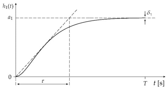
Figure 1. Step response of a first-order component.

Figure 2 shows the step response $h_2\left(t\right)$ for a second-order system defined by Equations (2) and (8), where

$${\omega }_0=\frac{2\mathsf{\pi }}{T_d\sqrt{1-\frac{{\ln }^2\left(\frac{\Delta y}{a_2}\right)}{{\left[\ln \left(\frac{\Delta y}{a_2}\right)\right]}^2+{\mathsf{\pi }}^2}}}$$

(12)

and:

$$\beta =\frac{-\ln \left(\frac{\Delta y}{a_2}\right)}{\sqrt{{\left[\ln \left(\frac{\Delta y}{a_2}\right)\right]}^2+{\mathsf{\pi }}^2}}$$

(13)

while $T_d,$ $\Delta y$ and ${\delta }_2$ are the period of damped natural vibrations, overshoot and margin of the steady-state for the corresponding step response, respectively [28].

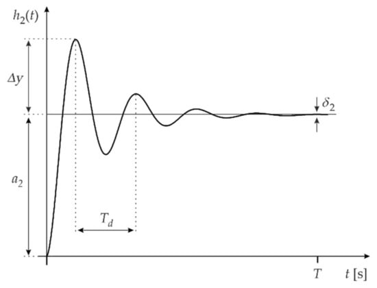
Figure 2. Step response of a second-order component.

The step responses $h_1\left(t\right)$ and $h_2\left(t\right)$ move exponentially toward and oscillate around the values of $a_1$ and $a_2,$ respectively. These step responses are characteristic of most components of the EPS. It is noteworthy that the step response includes the most information referring to the dynamics of EPS components before it achieves the steady-state [31].

Figure 3 shows the block diagram of the procedure for the preliminary modeling of the EPS components based on the IRNs.

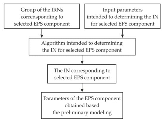
Figure 3. Block diagram of the procedure for the preliminary modeling of EPS components.

The procedure for the preliminary modeling is implemented based on the IRN group corresponding to the selected EPS component and the input parameters needed to determine the IN. The IRN group, in the first stage, is established for predefined ranges, which may include the expected parameters of the above component. The next stage involves the use of the selected algorithm, by which the IN is determined by comparing it with the IRN group. This comparison should aim at minimizing the specific error criterion. The mean-square criterion $\left(mse\right)$ is defined in this paper by the following formula:

$$mse=\sqrt{{\displaystyle \sum }_{i=0}^n{\left(Y_{i }-{Y^{\prime }}_i\right)}^2+{\displaystyle \sum }_{i=0}^n{\left(X_{i }-{X^{\prime }}_i\right)}^2},$$

(14)

where $Y_{i },$ ${Y^{\prime }}_i,$ $X_{i }$ and ${X^{\prime }}_i$ are the coordinate $Y$ for the determined IN, the coordinate $Y^{\prime }$ obtained for the IRN, the coordinate $X$ for the determined IN and the coordinate $X^{\prime }$ obtained for the IRN, respectively [31]. The above formula is applied below to validate the modeling results. In this way, the optimal shape of the IN is obtained. The parameters of the IRN that match it to the IN, with the minimal error, constitute a solution of the preliminary modeling of the considered EPS component.

3. Models for the Considered Electrical Machines

Below, we discuss the TF, IRNs and IN for the two most popular types of machines used in the EPSs, i.e., the squirrel-cage asynchronous (SCA) and brushless direct-current (BLDC).

3.1. The Squirrel-Cage Asynchronous Machine

The TF for the SCA is represented by the following formula [33,34]:

$$K_1\left(s\right)=k_{\mathrm{p}1}\frac{1+T_{\mathrm{z}}s}{\left(1+T_{1}s\right)\left(1+T_{2}s\right)}$$

(15)

where $T_1,$ $T_2$ and $T_{\mathrm{z}}$ are the time constants and $k_{\mathrm{p}1}$ is the gain factor. Equation (15) represents the second-order TF. The corresponding step response can be obtained by using Equation (3).

To establish the IRNs for above-mentioned machine, it is necessary to define the ranges for the parameters included in Equation (14). These ranges are determined intuitively so as to include the expected values of the above parameters. Hence, they were established as follows: $200.0–300.0 \mathrm{V}$ for $k_{\mathrm{p}1},$ $0.30–0.50 \mathrm{s}$ for $T_1,$ $0.250–0.450 \mathrm{s}$ for $T_2$ and $0.50–0.70 \mathrm{s}$ for $T_{\mathrm{z}}.$ The ranges of these parameters are typical for most SCA machines.

Figure 4 shows the group of IRNs for the above ranges. These IRNs were determined within the above ranges with the steps which are equal to $\Delta k_{\mathrm{p}1}=50.0 \mathrm{V}$ and $\Delta T_1=\Delta T_2=\Delta T_{\mathrm{z}}=0.10 \mathrm{s},$ by using the algorithm denoted as no. 1 (Table 1). The dotted line in Figure 4 indicates that it is the set of the IRNs with a number defined by the parameter ranges and the corresponding steps.

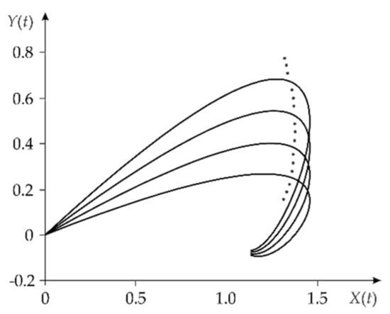
Figure 4. Group of IRNs for the SCA machine.

Figure 5 shows an example of a step response and the associated IN for the selected parameters: $k_{\mathrm{p}1}=303.0 \mathrm{V},T_1=0.430 \mathrm{s},$ $T_2=0.380 \mathrm{s}$ and $T_{\mathrm{z}}=0.750 \mathrm{s}$ [33] The time $T$ which corresponds to the steady-state is equal to 4.0 s.

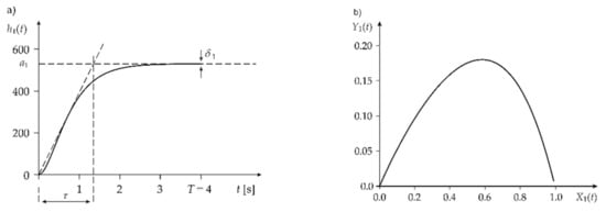
Figure 5. Example characteristics for the SCA machine: (a) step response; (b) IN.

The obtained step response corresponds to the time characteristic of the first-order system shown in Figure 1. The value of the $a_1$ parameter is calculated based on the formula:

$$a_1=k_{\mathrm{p}1}\left(1+T_{\mathrm{z}}\right)$$

(16)

and is equal to 530.3 V for ${\delta }_1=1\%$. The value of the $\tau$ parameter, which was obtained graphically, is equal to 1.38 s. The example of IN was obtained by using algorithm no. 1 (Table 1). The IN shown in Figure 5 (right panel) is matched to the group of IRNs, shown in Figure 4, by minimizing the mse, defined by Equation (14).

3.2. The Brushless Direct-Current Machine

The corresponding TF for the BLDC is

$$K_2\left(s\right)=\frac{k_{\mathrm{p}2}}{LJ{s}^2+RJs+2k_{\mathrm{p}2}{}^2},$$

(17)

where $k_{\mathrm{p}2}$ is the gain factor, $R$ and $L$ are the resistance and inductance of the machine circuit and $J$ is the moment of inertia [20,27]. The established ranges for the parameters included in Equation (15), which constitute the basis for determining the IRNs, are $5.0–15.0 \mathrm{V}$ for the factor $k_{\mathrm{p}2},$ $0.050–0.150 \mathsf{\Omega }$ for the resistance $R,$ $0.50–1.50 \mathrm{mH}$ for the inductance $L$ and $\left(1.0–3.0\right)\times {10}^{-3}$ $\mathrm{kg}·{\mathrm{m}}^2$ for the $J$ parameter. These ranges are predetermined in such a way as to cover most of the common parameters for the BLDC machine.

Figure 6 shows the group of IRNs for the above ranges. These IRNs were determined with the steps equal to: $\Delta k_{\mathrm{p}2}=5.0 \mathrm{V},$ $\Delta R=0.050 \mathsf{\Omega },$ $\Delta L=0.50 \mathrm{mH}$ and $\Delta J=1.0\times {10}^{-3}$ $\mathrm{kg}·{\mathrm{m}}^2,$ respectively, by using algorithm no. 1 (Table 1). The dotted line in Figure 6 determines the IRN group.

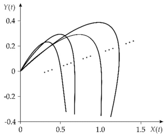
Figure 6. Group of IRNs for the BLDC machine.

The parameter values of both types of machine (SCA and BLDC), for which the IRNs were determined, are tabulated in Table 2.

Table 2. Parameters selected for the IRN determination.

SCA Machine				BLDC Machine
$k_{\mathrm{p}1} \left(\mathrm{V}\right)$	$T_1 \left(\mathrm{s}\right)$	$T_2 \left(\mathrm{s}\right)$	$T_{\mathrm{z}} \left(\mathrm{s}\right)$	$k_{\mathrm{p}2} \left(\mathrm{V}\right)$	$R \left(\mathsf{\Omega }\right)$	$L \left(\mathrm{mH}\right)$	$J \left(\mathrm{kg}·{\mathrm{m}}^2\right)$
200	0.30	0.250	0.50	5.0	0.050	0.50	0.0010
200	0.30	0.350	0.50	5.0	0.050	0.50	0.0020
200	0.30	0.450	0.50	5.0	0.050	0.50	0.0030
200	0.40	0.250	0.50	5.0	0.100	0.50	0.0010
200	0.40	0.350	0.50	5.0	0.100	0.50	0.0020
200	0.40	0.450	0.50	5.0	0.100	0.50	0.0030
200	0.50	0.250	0.50	5.0	0.150	0.50	0.0010
200	0.50	0.350	0.50	5.0	0.150	0.50	0.0020
200	0.50	0.450	0.50	5.0	0.150	0.50	0.0030
200	0.30	0.250	0.60	5.0	0.050	1.00	0.0010
200	0.30	0.350	0.60	5.0	0.050	1.00	0.0020
200	0.30	0.450	0.60	5.0	0.050	1.00	0.0030
200	0.40	0.250	0.60	5.0	0.100	1.00	0.0010
200	0.40	0.350	0.60	5.0	0.100	1.00	0.0020
200	0.40	0.450	0.60	5.0	0.100	1.00	0.0030
200	0.50	0.250	0.60	5.0	0.150	1.00	0.0010
200	0.50	0.350	0.60	5.0	0.150	1.00	0.0020
200	0.50	0.450	0.60	5.0	0.150	1.00	0.0030
200	0.30	0.250	0.70	5.0	0.050	1.50	0.0010
200	0.30	0.350	0.70	5.0	0.050	1.50	0.0020
200	0.30	0.450	0.70	5.0	0.050	1.50	0.0030
200	0.40	0.250	0.70	5.0	0.100	1.50	0.0010
200	0.40	0.350	0.70	5.0	0.100	1.50	0.0020
200	0.40	0.450	0.70	5.0	0.100	1.50	0.0030
200	0.50	0.250	0.70	5.0	0.150	1.50	0.0010
200	0.50	0.350	0.70	5.0	0.150	1.50	0.0020
200	0.50	0.450	0.70	5.0	0.150	1.50	0.0030
250	0.30	0.250	0.50	10.0	0.050	0.50	0.0010
250	0.30	0.350	0.50	10.0	0.050	0.50	0.0020
250	0.30	0.450	0.50	10.0	0.050	0.50	0.0030
250	0.40	0.250	0.50	10.0	0.100	0.50	0.0010
250	0.40	0.350	0.50	10.0	0.100	0.50	0.0020
250	0.40	0.450	0.50	10.0	0.100	0.50	0.0030
250	0.50	0.250	0.50	10.0	0.150	0.50	0.0010
250	0.50	0.350	0.50	10.0	0.150	0.50	0.0020
250	0.50	0.450	0.50	10.0	0.150	0.50	0.0030
250	0.30	0.250	0.60	10.0	0.050	1.00	0.0010
250	0.30	0.350	0.60	10.0	0.050	1.00	0.0020
250	0.30	0.450	0.60	10.0	0.050	1.00	0.0030
250	0.40	0.250	0.60	10.0	0.100	1.00	0.0010
250	0.40	0.350	0.60	10.0	0.100	1.00	0.0020
250	0.40	0.450	0.60	10.0	0.100	1.00	0.0030
250	0.50	0.250	0.60	10.0	0.150	1.00	0.0010
250	0.50	0.350	0.60	10.0	0.150	1.00	0.0020
250	0.50	0.450	0.60	10.0	0.150	1.00	0.0030
250	0.30	0.250	0.70	10.0	0.050	1.50	0.0010
250	0.30	0.350	0.70	10.0	0.050	1.50	0.0020
250	0.30	0.450	0.70	10.0	0.050	1.50	0.0030
250	0.40	0.250	0.70	10.0	0.100	1.50	0.0010
250	0.40	0.350	0.70	10.0	0.100	1.50	0.0020
250	0.40	0.450	0.70	10.0	0.100	1.50	0.0030
250	0.50	0.250	0.70	10.0	0.150	1.50	0.0010
250	0.50	0.350	0.70	10.0	0.150	1.50	0.0020
250	0.50	0.450	0.70	10.0	0.150	1.50	0.0030
300	0.30	0.250	0.50	15.0	0.050	0.50	0.0010
300	0.30	0.350	0.50	15.0	0.050	0.50	0.0020
300	0.30	0.450	0.50	15.0	0.050	0.50	0.0030
300	0.40	0.250	0.50	15.0	0.100	0.50	0.0010
300	0.40	0.350	0.50	15.0	0.100	0.50	0.0020
300	0.40	0.450	0.50	15.0	0.100	0.50	0.0030
300	0.50	0.250	0.50	15.0	0.150	0.50	0.0010
300	0.50	0.35	0.50	15.0	0.150	0.50	0.0020
300	0.50	0.450	0.50	15.0	0.150	0.5	0.0030
300	0.30	0.250	0.60	15.0	0.050	1.00	0.0010
300	0.30	0.350	0.60	15.0	0.050	1.00	0.0020
300	0.30	0.450	0.60	15.0	0.050	1.00	0.0030
300	0.40	0.250	0.60	15.0	0.100	1.00	0.0010
300	0.40	0.350	0.60	15.0	0.100	1.00	0.0020
300	0.40	0.450	0.60	15.0	0.100	1.00	0.0030
300	0.50	0.250	0.60	15.0	0.150	1.00	0.001
300	0.50	0.350	0.60	15.0	0.150	1.00	0.0020
300	0.50	0.450	0.60	15.0	0.150	1.00	0.0030
300	0.30	0.250	0.70	15.0	0.050	1.50	0.0010
300	0.30	0.350	0.70	15.0	0.050	1.50	0.0020
300	0.30	0.450	0.70	15.0	0.050	1.50	0.0030
300	0.40	0.250	0.70	15.0	0.100	1.50	0.0010
300	0.40	0.350	0.70	15.0	0.100	1.50	0.0020
300	0.40	0.450	0.70	15.0	0.100	1.50	0.0030
300	0.50	0.250	0.70	15.0	0.150	1.50	0.0010
300	0.50	0.350	0.70	15.0	0.150	1.50	0.0020
300	0.50	0.450	0.70	15.0	0.150	1.50	0.0030

Figure 7 shows the example step response and corresponding IN for the following parameters: $k_{\mathrm{p}2}=10.0 \mathrm{V},$ $R=0.10 \mathsf{\Omega },$ $L=1.0 \mathrm{mH}$ and $J=3.0\times {10}^{-3} \mathrm{kg}·{\mathrm{m}}^2$ [27]. The time $T$ which corresponds to the steady-state is equal to 125.0 ms.

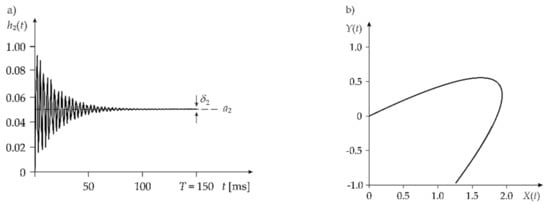
Figure 7. Example characteristics for the BLDC machine: (a) step response; (b) IN.

The obtained step response corresponds to the time characteristic of the second-order system shown in Figure 2. The value of the $a_2$ parameter is calculated using the following Equation

$$a_2=\frac{1}{2k_{\mathrm{p}2}}$$

(18)

and is equal to 0.050 V for ${\delta }_2=1\%$. The values of the $\Delta y$ and $T_d$ parameters are 0.0420 V and 5.80 ms, respectively. The example IN was obtained by using algorithm no. 1 (Table 1). In the same way, as for an SCA machine, the IN is matched to the group of IRNs shown in Figure 7, by minimizing the mse.

4. Example of Application

To implement the considered procedure, in accordance with the block diagram shown in Figure 3, a computational program using Microsoft Visual Studio 2019 Community was developed. This program can be applied to obtain the best match the determined IN to the group of IRNs with the minimum value of the $mse.$ The IRN groups equal to 81 were created for both types of machines.

Figure 8 shows the block diagram for the developed computer program which is intended for the preliminary modeling of the EPS components by using the EMs as an example.

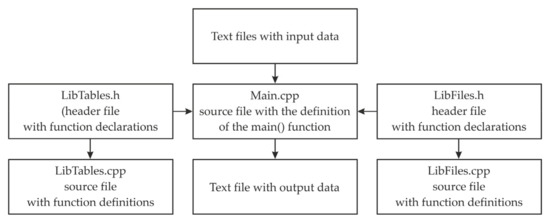
Figure 8. Block diagram of the developed computer program.

Text files with input data are loaded into the function main() which controls the entire program. This function is contained in the file Main.cpp. Additionally, the following header files are included in the above file:

• LibFiles.h: this file contains declarations of functions necessary to support operations on text files and a function declaration (together with the main algorithm) that determines the best match between the searched IN and the IRN group, with the minimum value of the $mse.$
• LibTables.h: this file contains declarations of functions that are necessary to support operations on two-dimensional dynamic arrays, which store input data read from text files.

The above-mentioned header files are also included with the following source files:

• LibFiles.cpp: this file contains definitions of the functions declared in the header file LibFiles.h.
• LibTables.cpp: this file contains definitions of the functions declared in the header file LibTables.h.

The results are saved to the text file after the entire program’s execution.

As a result of the research, the following parameters were obtained for both considered models of the EMs:

• SCA machine:

$k_{\mathrm{p}1}=240.0 \mathrm{V},T_1=0.270 \mathrm{s},$ $T_2=0.380 \mathrm{s}$ and $T_{\mathrm{z}}=0.580$ $\mathrm{s}.$

• BLDC machine:

$k_{\mathrm{p}2}=20.0 \mathrm{V},$ $R=0.70 \mathsf{\Omega },$ $L=2.0 \mathrm{mH}$ and $J=0.110 \mathrm{kg}·{\mathrm{m}}^2$.

Figure 9 shows the shapes of the IN (dotted line) and the corresponding IRN (solid line) obtained for the SCA (a) and BLDC (b) machines.

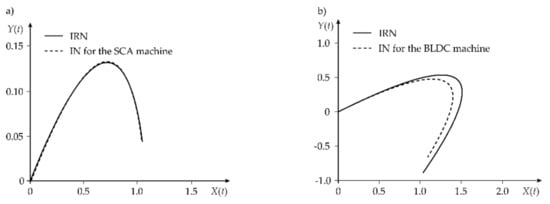
Figure 9. The shapes of the nets obtained for both machines: (a) IN; (b) IRN.

The shapes of the IN obtained for the SCA and BLDC machines match the corresponding IRNs with the $mse$ equal to 0.1527 and 1.6437, respectively.

The machine parameters corresponding to both IRNs are as follows:

• SCA machine

$k_{\mathrm{p}1}=250.0 \mathrm{V},T_1=0.50 \mathrm{s},$ $T_2=0.250 \mathrm{s}$ and $T_{\mathrm{z}}=0.70 \mathrm{s}.$

• BLDC machine:

$k_{\mathrm{p}2}=5.0 \mathrm{V},$ $R=0.150 \mathsf{\Omega },$ $L=0.50 \mathrm{mH}$ and $J=0.0030 \mathrm{kg}·{\mathrm{m}}^2$.

Figure 10 shows the characteristics of the $mse$ in the function of IRN number denoted by $i$ for the SCA (left panel) and BLDC (right panel) machines. The mse represents the accuracy of the considered models for both machines. The successive value of the $i$ parameter corresponds to the next row from Table 2.

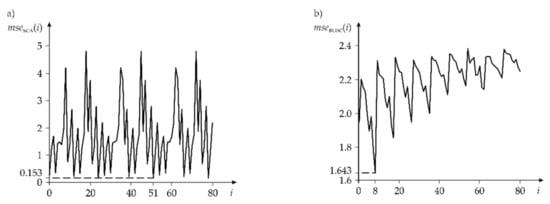
Figure 10. Characteristics of the $mse$ for the considered machines: (a) SCA; (b) BLDC.

The minimum values of the $mse$ were obtained for $i$ equal to 51 and 8, respectively, for both machines.

The shape of the INs for both machines and the $mse$ were determined by using a personal computer with an Intel Core i5 processor and 8 GB of RAM, as well as a maximum turbo frequency equal to 3.6 GHz.

5. Validation of the Proposed Method

The validation of the accuracy of the proposed method can only be justified when checking the influence of the used number of significant digits during the process of calculating mse for both considered machines. The assessment of the accuracy of matching the shapes of the IN to corresponding IRN is not necessary, as the proposed method is only the preliminary modeling of the EPS components for other methods of high accuracy, e.g., for those based on artificial intelligence. However, this preliminary method allows for efficient determination of approximate model parameters, which then can be used as the input data for the high accuracy methods.

Let us consider the validation of the proposed method as the relationship between the number of decimal places, when generating the particular points of the IN for both machines, and the mse defined by Equation (14). The numbers from 1 to 6 decimal places were considered for the validation. The comparison of the error values was also performed with the accuracy of 6 decimal places. The results which represent the relationship between the number of decimal places and the mse are tabulated in Table 3 for the SCA and BLDC machines.

Table 3. Validation of the proposed method.

	Value of mse
No.	SCA Machine	BLDC Machine
1	0.323607	1.801897
2	0.182069	1.644108
3	0.153032	1.644155
4	0.152622	1.643621
5	0.152622	1.643637
6	0.152622	1.643637

To conclude, based on the obtained results of the mse, the accuracy of calculations up to 4 decimal places is sufficient for the SCA machine, while the accuracy of calculations should be equal to 5 decimal places for the BLDC machine. This corresponds to 4 and 6 significant digits for the SCA and BLDC machines, respectively.

Figure 11 shows the shapes of the IN and the corresponding IRN obtained for one decimal place of accuracy (the first number in Table 2). The sixth number in Table 2 corresponds to the shapes of the IN and corresponding IRN shown in Figure 9.

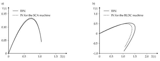
Figure 11. The shape of the nets for one decimal place of accuracy obtained for the SCA machine: (a) IN; (b) IRN.

Based on a comparison of the shapes of the IN and the corresponding IRN from Figure 9 and Figure 11, it is possible to confirm the difference between the mse for the first and sixth number from Table 3. The difference is equal approximately to 110% and 10% for the SCA and BLDC machines, respectively. This is definitely more for the SCA machine. Hence, for this machine it is more important to provide the appropriate accuracy of calculations than for the BLDC machine.

6. Conclusions

This paper presents simulation studies involving the preliminary modeling of EPS components using two types of EMs as an example, i.e., the SCA and BLDC machines. For the predetermined value of the TF parameters for both machines, the procedure intended to match the corresponding INs to the group of IRNs, with minimal value of error, was tested. The group of IRNs with numbers equal to 81, were determined symmetrically for each parameter associated with the TFs. The number of IRN for both groups was assumed in advance.

Based on the conducted calculations, any conclusion regarding that the accuracy of matching the IN to the corresponding IRN depends on the number of elements of the IRN. It is also important to properly select the ranges of particular parameters based on which the IRNs are determined. These ranges should be defined in such a way as to ensure that they contain the parameters for the considered component of the EPS. Meeting this requirement, in particular, guarantees complete implementation of the proposed procedure.

In practical applications, the ranges for the particular parameters of the EPS components under consideration should be determined based on measurement experience or the modeling results included in the relevant datasheet. Based on such defined ranges, it is necessary to determine a predetermined group of IRNs. The IN, in turn, is determined by applying the step response obtained by using the measurement experiment. After matching (with minimal error) the IN to the proper IRN, the result of the preliminary modeling of the examined EPS component is obtained. The results of this modeling ensure the parameters assigned to the IRN that most closely matches (with the minimum $mse$) the IN associated with the examined EPS component. The parameters determined in this way are the basis for using advanced modeling algorithms of the highest accuracy in applying the artificial intelligence methods. The research results presented in this paper may contribute to increasing the effectiveness and accuracy of using artificial intelligence tools for the needs of, first of all, modeling and simulation of electrical machines, machine diagnostics and field modeling.

The method proposed here can be extended to a broader group of systems, not only electrical, but also mechanical or hydraulic ones. As a method of the preliminary modeling, it can contribute to increasing the effectiveness of advanced methods used in the above-mentioned areas.

Appendix A.1. Procedure of Dynamic Linearisation

If there is a non-linear relationship between the pair of input-output variables: (x,$y)$ and their derivatives, then we have:

$$f\left[x,\dot{x},\ddot{x},\dots ,x^m,y,\dot{y},\ddot{y},\dots ,y^n\right]=0, m\le n.$$

(A1)

where $m$ and $n$ are the order of numerator and denominator.

Expanding the functions $f$ into the Taylor series gives one function $\left(m+n+2\right)$ of the independent variables. Therefore, it can be assumed that Equation (A1) describes a surface in the coordinate system of $\left(m+n+2\right)$ dimensional, which includes the static point $s_0$ with the coordinates $\left(x_0,y_0\right)$.

The typical procedure of dynamic linearisation includes two main stages:

• Comparison to zero of all derivatives for the variables $x$ and $y$ occurring in Equation (A1):

  $$f\left[x,0,0,\dots ,0,y,0,0,\dots ,0\right]=0.$$

  (A2)

which must also be met for the static point $\left(x_0,y_0\right)$:

$$f\left[x_0,0,0,\dots ,0,y_0,0,0,\dots ,0\right]=0.$$

(A3)

2.

Expanding the functions $f$ into the Taylor series around the static point $\left(x_0,y_0\right)$:

$$\begin{gathered} f\left[x,\dot{x},\ddot{x},\dots ,x^m,y,\dot{y},\ddot{y},\dots ,y^n\right]=f\left[x_0,0,0,\dots ,0,y_0,0,0,\dots ,0\right]+{\left.\frac{\partial f}{\partial x}\right|}_{s_0}\left(x-x_0\right)+. \\ {\left.+\frac{\partial f}{\partial \dot{x}}\right|}_{s_0}\left(\dot{x}-0\right)+\dots +{\left.\frac{\partial f}{\partial x^m}\right|}_{s_0}\left(x^m-0\right)+{\left.\frac{\partial f}{\partial \mathrm{y}}\right|}_{s_0}\left(y-y_0\right){\left.+\frac{\partial f}{\partial \dot{y}}\right|}_{s_0}\left(\dot{y}-0\right)+. \\ +\dots +{\left.\frac{\partial f}{\partial y^n}\right|}_{s_0}\left(y^n-0\right)+N,. \end{gathered}$$

(A4)

where $N$ denotes the nonlinear components occurring in the expansion of Taylor series for the function $f.$

After rejection from Equation (A4) of the nonlinear components and taking Equations (12) and (13) into account, we have:

$$\begin{gathered} {\left.\frac{\partial f}{\partial x}\right|}_{s_0}\left(x-x_0\right)+{\left.\frac{\partial f}{\partial \dot{x}}\right|}_{s_0}\dot{x}+\dots +{\left.\frac{\partial f}{\partial x^m}\right|}_{s_0}{x}^m+. \\ +{\left.\frac{\partial f}{\partial \mathrm{y}}\right|}_{s_0}\left(y-y_0\right){\left.+\frac{\partial f}{\partial \dot{y}}\right|}_{s_0}\dot{y}+\dots +{\left.\frac{\partial f}{\partial y^n}\right|}_{s_0}{y}^n=0. \end{gathered}$$

(A5)

Equation (A5) is the is a linearised equation with constant coefficients around the point $s_0$ for a dynamic system defined by Equation (A1).

References

- Boldea, I. Electric Generators and Motors: An Overview. China Electrotech. Soc. Trans. Electr. Mach. Syst. 2017, 1, 3–14. [Google Scholar] [CrossRef]
- Zhang, H.; Cao, D.; Du, H. Modeling, Dynamics and Control of Electrified Vehicles; Elsevier: Amsterdam, The Netherlands, 2018; ISBN 978-0-12-812786-5. [Google Scholar]
- Michaud, B.; Begon, M. Two Efficient Static Optimization Algorithms that Account for Muscle-Tendon Equilibrium: Ap-proaching the Constraint Jacobian via a Constant or a Cubic Spline Function. Comput. Methods Biomech. Biomed. Engin. 2020, 23, 703–709. [Google Scholar] [CrossRef] [PubMed]
- Arslan, M.; Çunkaş, M.; Sağ, T. Determination of Induction Motor Parameters with Differential Evolution Algorithm. Neural Comput. Appl. 2011, 21, 1995–2004. [Google Scholar] [CrossRef]
- Michalewicz, Z. The Emperor is Naked: Evolutionary Algorithms for Real-World Applications. ACM Ubiquity 2012, 3, 1–13. [Google Scholar]
- Avalos, O.; Cuevas, E.; Gálvez, J. Induction Motor Parameter Identification Using a Gravitational Search Algorithm. Comput. 2016, 5, 6. [Google Scholar] [CrossRef]
- Lei, G.; Zhu, J.; Guo, Y.; Liu, C.; Ma, B. A Review of Design Optimization Methods for Electrical Machines. Energies 2017, 10, 1962. [Google Scholar] [CrossRef]
- Jiang, X.; Chen, L.; Xu, X.; Cai, Y.; Li, Y.; Wang, W. Analysis and Optimization of Energy Efficiency for an Electric Vehicle with Four Independent Drive In-Wheel Motors. Adv. Mech. Eng. 2018, 10, 1–9. [Google Scholar] [CrossRef]
- Turk, N. Diagnosis of Mechanical Faults in Electric Motors. Int. J. Electr. Comput. Eng. 2016, 8, 1–6. [Google Scholar]
- Sahoo, S.; Rodriguez, P.; Sulowicz, M. Evaluation of Different Monitoring Parameters for Synchronous Machine Fault Diagnostics. Electr. Eng. 2016, 99, 551–560. [Google Scholar] [CrossRef]
- Dineva, A.; Mosavi, A.; Gyimesi, M.; Vajda, I.; Nabipour, N.; Rabczuk, T. Fault Diagnosis of Rotating Electrical Machines Using Multi-Label Classification. Appl. Sci. 2019, 9, 5086. [Google Scholar] [CrossRef]
- Coronado, P.D.U.; Ahuett-Garza, H. Control Strategy for Power Distribution in Dual Motor Propulsion System for Electric Vehicles. Math. Probl. Eng. 2015, 2015, 814307. [Google Scholar] [CrossRef]
- Merabet, A. Advanced Control for Electric Drives: Current Challenges and Future Perspectives. Electronics 2020, 9, 1762. [Google Scholar] [CrossRef]
- Stefanski, T.; Zawarczynski, Ł. Parametric Identification of the DC Brushless Motor Mathematical Model. PAK 2011, 57, 109–112. [Google Scholar]
- Chapman, J. Electric Machinery Fundamentals; McGraw-Hill: Singapore, 2011; pp. 357–447. ISBN 0073529540. [Google Scholar]
- Caruso, M.; di Tommaso, A.O.; Lisciandrello, G.; Mastromauro, R.A.; Miceli, R.; Nevoloso, C.; Spataro, C.; Trapanese, M. A General and Accurate Measurement Procedure for the Detection of Power Losses Variations in Permanent Magnet Synchro-nous Motor Drives. Energies 2020, 13, 1–19. [Google Scholar] [CrossRef]
- Giordano, D.; Signorino, D.; Gallo, D.; Brom, H.E.V.D.; Sira, M. Methodology for the Accurate Measurement of the Power Dissipated by Braking Rheostats. Sensors 2020, 20, 6935. [Google Scholar] [CrossRef]
- Xiang, C.; Wang, X.; Ma, Y.; Xu, B. Practical Modeling and Comprehensive System Identification of a BLDC Motor. Math. Probl. Eng. 2015, 2015, 879581. [Google Scholar] [CrossRef]
- Fico, V.M.; Vázquez, A.L.R.; Prats, M.; Ángeles, M.; Bernelli-Zazzera, F. Failure Detection by Signal Similarity Measurement of Brushless DC Motors. Energies 2019, 12, 1364. [Google Scholar] [CrossRef]
- Shin, C.; Choi, C.; Lee, W. Advance Angle Calculation for Improvement of the Torque-to-Current Ratio of Brushless DC Motor Drives. Energy Procedia 2012, 14, 1410–1414. [Google Scholar] [CrossRef][Green Version]
- Huang, C.; Lei, F.; Han, X.; Zhang, Z. Determination of Modeling Parameters for a Brushless DC Motor That Satisfies the Power Performance of an Electric Vehicle. Meas. Control. 2019, 52, 765–774. [Google Scholar] [CrossRef]
- Mytnikov, A.V.; Lavrinovich, V.A.; Evseeva, A.M.; Stepanov, I.A. Development of Advanced Winding Condition Control Technology of Electric Motors Based on Pulsed Method. Resour. Technol. 2017, 3, 232–235. [Google Scholar] [CrossRef]
- Wu, R.C.; Tseng, Y.W.; Chen, C.Y. Estimating Parameters of the Induction Machine by the Polynomial Regression. Appl. Sci. 2018, 8, 1–13. [Google Scholar] [CrossRef]
- Ćalasan, M.; Micev, M.; Ali, Z.M.; Zobaa, A.F.; Aleem, S.H.E.A. Parameter Estimation of Induction Machine Single-Cage and Double-Cage Models Using a Hybrid Simulated Annealing–Evaporation Rate Water Cycle Algorithm. Mathematics 2020, 8, 1024. [Google Scholar] [CrossRef]
- Rajagopalan, S.; Restrepo, J.; Aller, J.; Habetler, T.G.; Harley, R. Selecting Time-frequency Representations for Detecting Rotor Faults in BLDC Motors Operating under Rapidly Varying Operating Conditions. In Proceedings of the 31st Annual Conference of IEEE Industrial Electronics Society, IECON 2005, Raleigh, NC, USA, 6–10 November 2005; p. 6. [Google Scholar]
- Enesi, Y.A.; Zungeru, A.M.; Abraham-Attah, P.O.; Ademoh, I.A. Analysis of Power Flowand Torque of Asynchronous Induc-tion Motor Equivalent Circuits. Int. J. Adv. Sci. Technol. 2013, 6, 713–732. [Google Scholar]
- Karthik, K.; Kumar, R.K.; Sreenivasulu, P. Modeling and Performance Analysis of BLDC Motor under Different Operating Speed Conditions. Int. J. Eng. Comput. Sci. 2017, 6, 21468–21475. [Google Scholar]
- Li, M.; Chen, Q.; Liu, Y.; Ding, Y.; Xie, H. Modelling and Experimental Verification of Step Response Overshoot Removal in Electrothermally-Actuated MEMS Mirrors. Micromachines 2017, 8, 1–11. [Google Scholar] [CrossRef]
- Belaid, K.A.; Belahrach, H.; Ayad, H. Numerical Laplace Inversion Method for Through-Silicon Via (TSV) Noise Coupling in 3D-IC Design. Electronics 2019, 8, 1–21. [Google Scholar] [CrossRef]
- Wesolowski, J. Determination of Linear Object Dynamics Class and Conception of Template Identification Net Construction. In Proceedings of the Modelling, Identification and Control 2005, Insbruck, Austria, 16–18 February 2005. [Google Scholar]
- Pandey, A.; Gregory, J.W. Step Response Characteristics of Polymer/Ceramic Pressure-Sensitive Paint. Sensors 2015, 15, 1–21. [Google Scholar] [CrossRef] [PubMed]
- Westphal, L.C. Linearization Methods for Nonlinear Systems; Springer Science + Business Media: New York, NY, USA, 2001; ISBN 978-1-4613-5601-1. [Google Scholar]
- Lin, C.H. Altered Grey Wolf Optimization and Taguchi Method with FEA for Six-Phase Copper Squirrel Cage Rotor Induction Motor Design. Energies 2020, 13, 1–17. [Google Scholar] [CrossRef]
- Soomro, A.; Amiryar, M.E.; Nankoo, D.; Pullen, K.R. Performance and Loss Analysis of Squirrel Cage Induction Machine Based Flywheel Energy Storage System. Appl. Sci. 2019, 9, 4537. [Google Scholar] [CrossRef]
Publisher’s Note: MDPI stays neutral with regard to jurisdictional claims in published maps and institutional affiliations. |
© 2021 by the authors. Licensee MDPI, Basel, Switzerland. This article is an open access article distributed under the terms and conditions of the Creative Commons Attribution (CC BY) license (https://creativecommons.org/licenses/by/4.0/).