1. Introduction
Electric rail transport is one of the most popular forms of public urban transport, due to its cost-effectiveness and low carbon footprint. Various technical and other measures are being taken to further increase the energy efficiency of electric rail transport, such as timetable optimization, reversible substations, eco driving, regenerative braking, etc., with regenerative braking being the method with the greatest energy saving potential [
1]. In papers [
2,
3,
4], the possibilities of using regenerative braking energy to increase the energy efficiency of rail vehicles are considered. Electric rail vehicles convert kinetic energy into electrical energy during braking, i.e., regenerative braking takes place when the electric motor operates in generator mode. The electricity generated in this way can be fed back into the power grid, dissipated on the braking resistors, or stored for further use. Regenerative braking is not possible with certain power supply grids and can also lead to impermissible overvoltages in the supply voltage. If the supply network cannot receive energy, the braking energy is dissipated at the braking resistors and irreversibly converted into thermal energy. The most efficient way to use braking energy is to store it and then use it in a regenerative braking system.
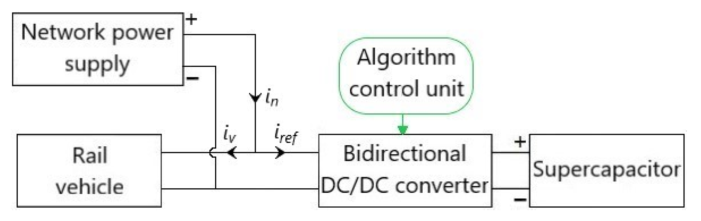
The regenerative braking systems consist of an energy storage system, a bidirectional DC converter, and an algorithm for energy flow control. In [
5], the possibilities of energy conservation by energy storage systems (ESS) are considered in general. The ESS can be located outside the vehicle (wayside energy storage) or inside the vehicle as a mobile energy storage system (onboard energy storage). The work, [
6], deals with the optimal positioning and sizing of a stationary ESS, while the studies in [
7] analyze the economic and energetic viability of installing an ESS into a rail vehicle. The ESS usually consists of battery or supercapacitor modules; in rare cases, flywheels are also used [
8]. Battery packs are characterized by high energy density but low power density and relatively low number of charge and discharge cycles [
9,
10]. Supercapacitor storages have high power density and a large number of cycles, but relatively low energy density [
11,
12]. Due to the frequent cycling of large amounts of power in electric rail vehicles, it is more convenient to use supercapacitors to store braking energy. The bidirectional DC/DC converter connects the DC link of the vehicle’s main drive converter to the ESS and its topology depends on the type of vehicle and the ESS used. A survey of existing topologies of DC converter used for this purpose is discussed in detail in [
13,
14,
15,
16]. The power management algorithm monitors the filling and emptying of the storage depending on the current state of charge, state of the vehicle, and the selected control algorithm, which can be maximum energy saving, preservation of the lifetime of the ESS, stabilization of the power grid, etc.
In the literature, different variants of the energy flow control algorithm within the regenerative braking system are mentioned. In [
17], the case of integrating a battery and a supercapacitor in a tram and optimizing the speed profile, depending on the known data about the operation of traffic lights, is considered in order to increase the energy efficiency and the travel time. By applying this algorithm, about 22.3% energy saving is achieved. In [
18], the authors use dynamic control of charge and discharge thresholds of stationary supercapacitor, ESS, to minimize energy dissipation at the braking resistor and maximize energy savings. The results show that changing the thresholds dynamically enables higher energy storage efficiency even when multiple vehicles are connected to the same sector of the utility grid. In [
19], the optimal sizing of a stationary energy storage system is considered, where the main objective is to stabilize the power grid voltage, but the focus of the work is not on increasing the efficiency or maintaining the lifetime of the ESS. In [
20], a simplified optimization of the charging threshold is described. The mean charging threshold is calculated offline as a result of optimizing energy consumption of wayside ESS with a 15% energy reduction and a 38% reduction peak voltage value. In [
21], a genetic optimization algorithm is used to try to equalize the frequency of use of a large number of ESS within a power grid to compensate for the aging of a single storage device. In [
22], dynamic programming is used to estimate the maximum possible energy savings, i.e., the process of dividing the system in a number of smaller parts in order to simplify the solution. Due to the dependence of the energy saving on the a priori selection of the weight coefficients within the optimization process, the amount of energy saving varies, as well as the number of cycles used. An algorithm that maximizes the saved energy at the substations is described in [
23]. Using onboard energy storage, in order to reduce peak power demand while using a genetic algorithm resulting in an energy saving of 15.56% and peak power reduction of 63.49%. In [
24], an integrated optimization algorithm, aiming to reduce energy consumption, is presented for metro trains. The speed profile, headway, and interstation runtime are the variables used in the Non-Dominant Gravitational Search Algorithm (NS-GSA), which also takes into account the downhill drive of the metro train. More complex optimization methods, such as particle swarm optimization [
25], and controlling techniques [
26] can be used in order to further enhance energy savings and power grid stability in real-time, but depend mainly on the available computing power inside the rail vehicle.
The algorithms in the previously cited papers do not take into account the influence of the vertical profile and the slope of the vehicle route during storage or use of braking energy. Driving uphill necessitates higher drive currents in order to compensate gravitational forces, which can negatively impact the power grid’s stability. Driving downhill generates more regenerative energy which can be stored or sent back to the grid, but sending back too much energy also impacts negatively the power grid’s stability. Consequently, this paper presents an algorithm for controlling a tram regenerative braking system with a supercapacitor module (SC) as an energy storage, which increases the energy efficiency of the vehicle and reduces the impact of the vehicle on the supply network. The algorithm stands out because it takes into account the influence of gravitational force on the vehicle, while still providing energy savings and increased grid stability despite driving uphill and downhill and being subject to urban traffic with automobiles. The algorithm is presented in two variants: the minimum energy variant minimizes the energy taken from the power grid, and the minimum gradient which minimizes the number of peak currents over 1000 A. In the second chapter, mathematical models of the electric rail vehicle, power supply network, and supercapacitor storage are developed and integrated within the model of the entire system developed in the MATLAB programming environment. The third chapter presents the development of the energy flow control algorithm for optimizing power grid energy consumption and analyzes the charging and discharging scenarios of the supercapacitor module in different situations. The fourth chapter gives simulation results using the model of regenerative tram braking system with built-in proposed algorithm on routes of different vertical profile and slope, as well as the analysis of the obtained results.
3. Control Algorithm
3.1. Control Algorithm Objective
The objectives of the control algorithm are: (i) to minimize the energy used to supply the tram from the power grid and (ii) to reduce the peak current values of the grid by using the energy of regenerative braking. According to this algorithm, the regenerative braking energy is stored in the supercapacitor whenever the supercapacitor is not fully charged. The remaining energy that cannot be stored is dissipated at the braking resistor. Since the stored energy is not sufficient to reduce the peak loads during the entire trip, the possibility of recharging the supercapacitor module from the grid is also considered. It follows that the two main objectives of the control algorithm in terms of minimizing the total energy extracted from the grid are opposite to each other and it is necessary to find a balance between the criteria of increasing energy efficiency and reducing the impact on the grid.
Thus, the algorithm assumes the grid load is due to the vehicle drive and the load due to the recharging of the supercapacitor. The grid load from the vehicle traction depends on the current speed, the vehicle acceleration and the track slope. It will be shown that the grid load due to supercapacitor recharging also depends on the instantaneous vehicle speed and track slope, as well as the supercapacitor’s state of charge.
In addition to the direction of energy flow, the algorithm should determine the amounts of current with which the supercapacitor tank should be discharged and charged, i.e., it is necessary to define the reference current of a bidirectional DC/DC converter. During the discharge of the supercapacitor tank, the current of the supercapacitor tank should decrease as the state of charge decreases. This prevents a sudden load on the grid at the moment when the minimum state of charge of the supercapacitor is reached, i.e., the grid gradually takes over the entire load.
In the following subsection, the algorithm for controlling the energy flow during the discharge and charge of the ESS is described. Due to the influence of the instantaneous vehicle speed on the amount of energy required, the algorithm is divided into three areas: high, medium, and low kinetic energy zone.
3.2. Algorithm for Supercapacitor Discharge
3.2.1. High Kinetic Energy Zone
The zone of high kinetic energy is identified by the measured driving speed. If the speed is greater than the set threshold (
Vth), the vehicle is in the high kinetic energy zone. If further acceleration of the vehicle follows, the question arises whether the energy from the supercapacitor, or from the power grid, should be used to achieve a higher kinetic energy of the tram. The answer to this question is obtained by comparing the measured current that the vehicle draws from the grid with the defined current threshold (
Ith). In case the value of the vehicle current is smaller than the parameter
Ith, the vehicle current is provided by the power grid, i.e., the reference current of the bidirectional converter DC is zero. In case the value is greater than
Ith, part of the current to supply the vehicle is also given by the supercapacitor. In this case, it is necessary to determine the reference value of the supercapacitor discharge current. In addition to the reference current directions as in
Figure 1, one of the possible solutions is a negative magnitude of the current required to power the vehicle increased by the parameter
Ith, i.e.,:
It follows that the maximum value of the main current is kept at the value of the parameter,
Ith, and the rest is taken from the supercapacitor module. With this reference current, which must not exceed a maximum value because of the protection of the supercapacitor, there will be moments when the grid abruptly takes over the entire load when the state of charge of the supercapacitor reaches the minimum allowable value. To avoid this, a term is added to the expression to reduce the reference current as the state of charge of the supercapacitor reaches a minimum value. It is an exponential function and represents a new form of the reference current:
In Expression (1), it is assumed that this is a supercapacitor module with a maximum voltage of 500 V that is discharged to half of its capacity. The power in the exponential function ensures that the reference current decreases as the state of charge, i.e., the voltage
USC of the supercapacitor decreases. The numerator in the exponential function ensures that the supercapacitor empties the fastest when the state of charge is highest, while the parameter
kv affects the slope of the exponential function.
Figure 3 shows the influence of the parameter
kv on the magnitude of the exponential function.
Increasing the parameter,
kv, turns the exponential function into a line. In the case when
kv takes the value +∞, the value of the exponential function takes the value 1, i.e., the reference current becomes equal to the current defined according to expression (9).
Figure 4 shows a flow diagram of the reference current control algorithm for the high kinetic energy zone, where
.
In the high kinetic energy zone, the supercapacitor is not charged from the power grid, but only by regenerative braking (more on this in
Section 3.3).
3.2.2. Low Kinetic Energy Zone
In order to reduce the number of parameters in the optimization process (more details in
Section 4), the speed threshold between the low and medium kinetic energy zones was chosen to be the speed at which the tram kinetic energy is 3% of its maximum value. Assuming a maximum tram speed of 50 km/h, the speed threshold between low and medium kinetic energy is 8.7 km/h.
And the zone of low kinetic energy, given the current, is divided into two parts. If the tram current is greater than 100 A, the supercapacitor is discharged with the reference current:
The current limit of 100 A was chosen because it divides the zone of low kinetic energy into two equal parts, with respect to vehicle speed. Indeed, the speed of 8.7 km/h corresponds to the current of 200 A of the vehicle modeled in the next chapter. Discharging the supercapacitor in the low kinetic energy zone for currents greater than 100 A further reduces the load on the power grid. The parameter,
km, is used to determine the change in the slope of the exponential function. The goal is to discharge the supercapacitor module more slowly in this zone than in the high kinetic energy zone, i.e., to store some energy for future accelerations. This means that the parameter,
km, should be smaller than the parameter,
kv.
Figure 5 shows a flow diagram for the low kinetic energy zone, where
.
When the tram current is less than 100 A, the supercapacitor is charged from the grid. In this way, higher power grid loads are avoided during the next vehicle acceleration (more details in
Section 3.3).
3.2.3. Medium Kinetic Energy Zone
The zone of medium kinetic energy (in this particular case; 8.7 km/h <
v <
Vth) is the zone from which the algorithm can switch to the two zones of kinetic energy previously described, by accelerating or braking. The following expressions used for the reference discharge current:
In the previous cases, a constant positive value was added to the negative value of the current required for tram traction, and this sum was multiplied by the exponential function. This is not the case here, as the objective in this kinetic energy zone is not to keep the power grid current at a certain value, but to generally reduce the load on the grid.
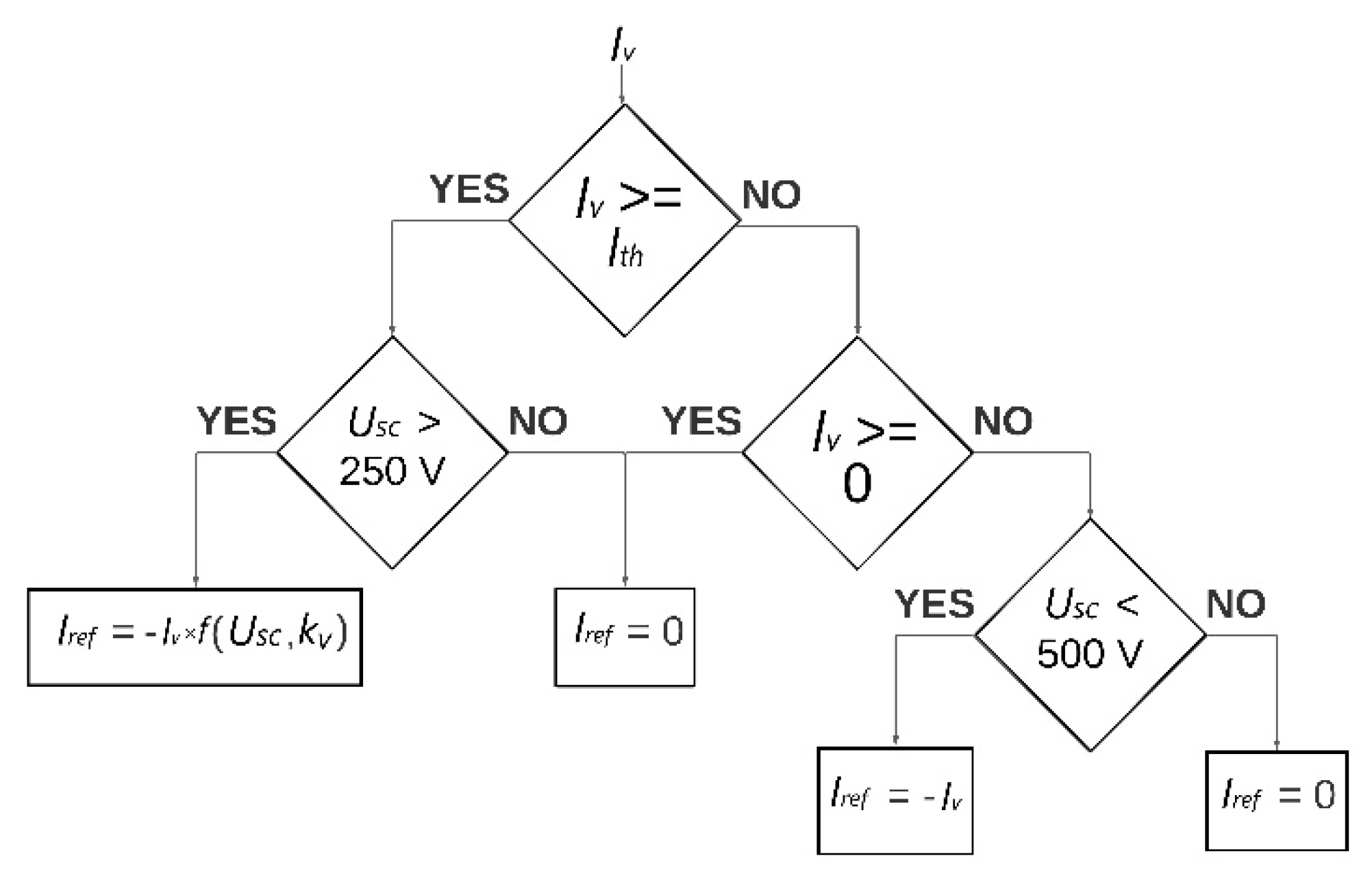
Figure 6 shows a flow chart for the zone of medium kinetic energy in which
.
In this zone also, it is permitted to recharge the supercapacitor from the power gird for any potential accelerations. Whether the supercapacitor is recharged from the grid or used to power the vehicle is determined by the parameter,
Vstop. The value of the parameter,
Vstop, starts from the value,
Vth, and decreases linearly to 8.7 km/h (the boundary between the medium and low kinetic energy zones) and is reset to the value of,
Vth, once the tram has arrived at the stop. The distance between stations in vector form was obtained using the application
Google Earth Pro in advance. As long as the vehicle speed is less than the
Vstop speed, the supercapacitor is recharged from the grid, otherwise it is used to power the vehicle drive.
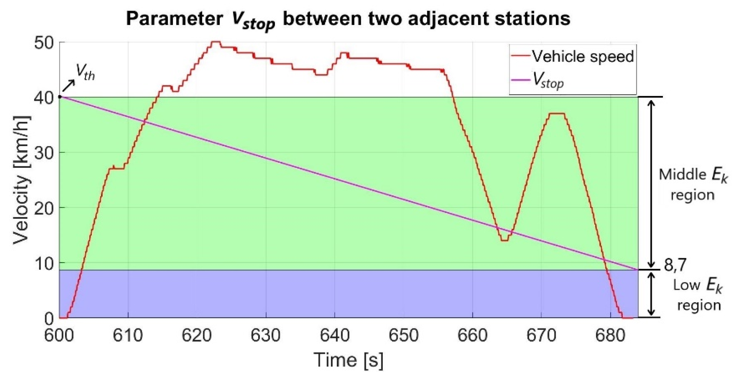
Figure 7 shows the change of the parameter,
Vstop, between two adjacent stations, where
Vth = 40 km/h is arbitrarily chosen. From the figure, it can be seen that initially the value of the parameter,
Vstop, is higher than the tram speed. According to the diagram in
Figure 6, this means that the supercapacitor is not emptied, but is refilled from the supply network towards the charging surface (more on this in
Section 3.3). Only when the driving speed exceeds the parameter,
Vstop, the supercapacitor is used to power the vehicle drive. Moreover, at the time of transition from the medium kinetic energy zone to the high kinetic energy zone, when very high currents occur, the supercapacitor has more energy available, so the peak current values of the power grid are lower. As the tram approaches the next stop, the value of the parameter,
Vstop, decreases, which means that the supercapacitor is allowed to charge less from the power grid because when the tram arrives at the stop, it is expected to brake, and thus regenerative braking energy is available for storage.
3.3. Algorithm for Supercapacitor Charge
As mentioned above, the supercapacitor is charged with regenerative braking energy and, if necessary, replenished with energy from the grid. The regenerative braking energy is always stored in the supercapacitor when it is not fully charged, regardless of the instantaneous kinetic energy of the tram, so this case is straightforward.
Figure 8 shows a flow diagram for storing regenerative braking energy for all speeds less than the parameter,
Vth. The regenerative braking energy is also stored for speeds greater than the parameter,
Vth, i.e., in the high kinetic energy zone. However, in the flow diagram for this zone, it is first checked whether the magnitude of the vehicle current is greater than the parameter,
Ith. If this condition is not met and the vehicle current is negative, the regenerative braking energy is stored in the supercapacitor.
The amount of current used to charge the tank from the power grid depends on the speed of the tram, i.e., kinetic energy, the difference in elevation between two adjacent stops, and the state of charge of the supercapacitor. The value of the charging current should be highest when the tram is at a standstill, the state of charge of the supercapacitor is minimal and the greatest possible difference in height between the two stops is to be expected. This value decreases when one of the parameters increases and should be zero at maximum state of charge regardless of other parameters.
Supercapacitor charging from the power grid is not considered at all in the case where the tram is in the high kinetic energy zone, since in this case the energy of future regenerative braking could not be stored. Therefore, supercapacitor charging in the high kinetic energy zone would contradict the goals towards which the control algorithm is currently being developed.
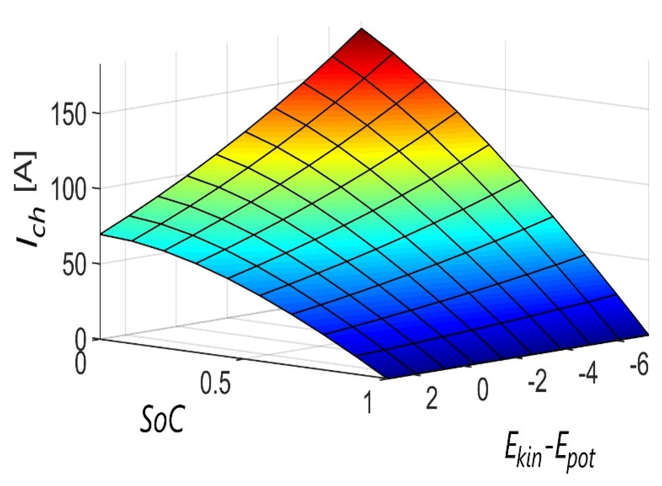
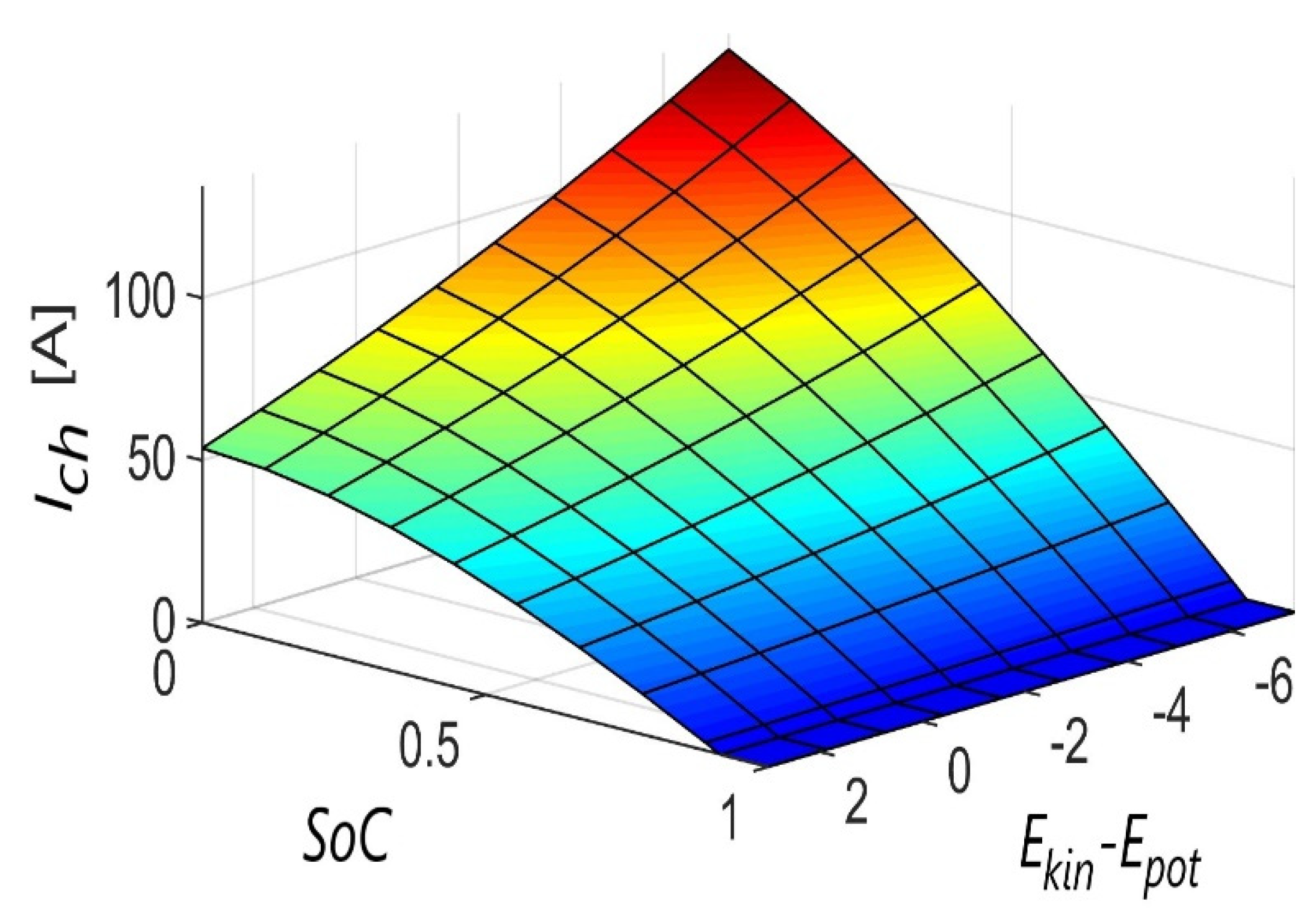
According to the previous considerations, a filling surface is defined with the following axes:
x-axis—the difference between the kinetic energy of the tram and the potential energy between two adjacent stations
y-axis—state of charge of the supercapacitor
z-axis—the magnitude of the charging current
The difference between the kinetic and potential energy (value on the x-axis) is a good indicator of the potential load on the power grid. For example, if the difference between the kinetic and potential energy is negative, then there is an uphill slope on the vehicle’s route, and it is desirable to charge the supercapacitor module with a higher current. On the other hand, if the value on the x-axis is positive and of high magnitude, it means that the tram is travelling at high speed and/or a descent follows on the vehicle route.
The magnitude of the charging current changes according to the following function:
The term
in (13) ensures that the charging current decreases as the difference between kinetic and potential energy increases. A value of −7.27 represents the scaled maximum negative value of potential energy, since the maximum difference in height between two adjacent stations for one of the track profiles considered in the simulation experiment is approximately 15 m. The term,
, ensures that the charging current decreases as the state of charge increases. The term,
makes sure that the function goes to 0 when the state of charge reaches the value, a
3. For this reason, the parameter, a
3, is constrained between the values, 0 and 1 (minimum and maximum state of charge). This kind of charging according to the defined function,
f (x,
y), coincides conceptually with the above objectives. In order to be able to define the general form of such a surface, the parameters,
a1,
a2,
a3, and
a4 are introduced and determined by an optimization procedure. For better understanding, the charging surface for certain parameters (
a1 = 244.5654,
a2 = 0.0567,
a3 = 0.9997,
a4 = 0.1007) is shown in
Figure 9.
It can be seen from
Figure 9 that the maximum value of the charging current applies to the minimum state of charge of the supercapacitor and the minimum value of the difference between the kinetic and potential energy. It can also be seen that the charging current tends to zero when the state of charge reaches the maximum value.
Figure 10 shows a complete flow diagram of the control algorithm.
4. Simulation Experiment
In this chapter, the simulation results are presented with the parameters obtained through optimization. In the optimization, the algorithm, fminsearch, was used within the MATLAB/Simulink software tool for two criterion functions. For one function, the objective is to minimize the total energy taken from the grid (14), and for the other, the objective is to minimize the sum of the squares of the current gradient of the power grid
in (15):
The parameters determined with (14) and (15) are: Vth, Ith, kv, km, ks, a1, a2, a3, and a4. The optimization was performed on the data for line no. 14 of Zagreb Electric Tram uphill, as a more challenging scenario. The optimization results were also applied to the data for tram line No. 14 downhill and tram line no.11, which is mostly flat, with minimal ascents and descents.
In the rest of the chapter, after describing the other parameters of the model and the input variables in the model, we simulate and analyze: (i) power grid peak currents, (ii) supercapacitor energy, and (iii) energy from the power grid. For each of the lines, 4 sets of parameters for peak grid current, supercapacitor energy, and energy drawn from the power grid were determined according to the following criteria:
minimum energy from the grid with a current limitation of the supercapacitor module of 240 A
minimum energy from the network with a current limit of the supercapacitor module of 500 A
minimum sums of the square of the mains current gradient with the supercapacitor module current limit of 240 A
minimum sums of the square of the mains current gradient with the current limit of the supercapacitor module of 500 A
4.1. Simulation Model Inputs and Parameters
The parameters of the supercapacitor module are based on the datasheet of the commercial 125 V HEAVY TRANSPORTATION MODULE, manufactured by Maxwell [
30],
Table 1.
Table 2 contains the parameters of the tram TMK 2200_K, manufactured by Končar Elektroindustrija Zagreb and TŽV Gredelj d.o.o., and the parameters of the power grid.
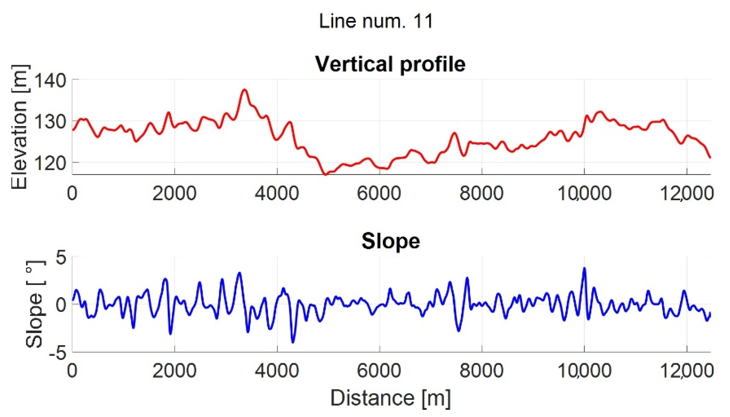
There are 15 tram lines in the urban area of Zagreb. Among them are lines no. 14 and No. 11. Line No. 14 is characterized by the fact that on a part of the track, a significant slope gradient appears in comparison with most other tram lines. This means that depending on the direction of travel by line No. 14, the power grid current profile varies in both directions compared to line No. 11. Of course, the current profile also depends on the speed and acceleration of the vehicle. The track elevation profile in vector form was obtained using the application, Google Earth Pro.
Figure 11 shows the vertical profile and gradient for line no. 11, and
Figure 12 for line No. 13.
Figure 13 shows the measured speed profile of the tram in line No. 14. The speed profile is also measured for the line No. 11. The speed profiles and track slope are the simulation inputs.
4.2. Simulation Results
4.2.1. Power Grid Current Peak Values
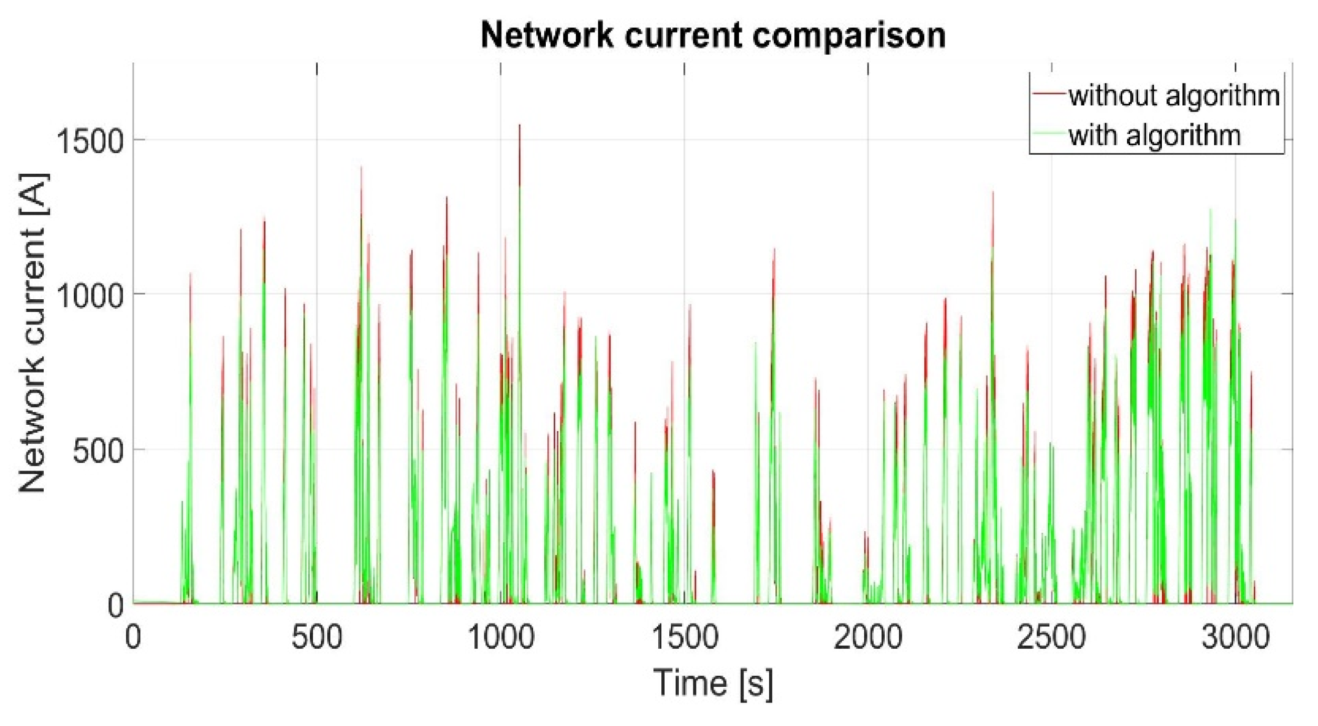
Figure 14 shows a comparison of the grid current with and without the control algorithm for the parameters determined according to the minimum energy criterion (14) with a supercapacitor current limit of 240 A for the tramline No. 14. The simulation results show that the grid current without the supercapacitor storage system and use of regenerative braking energy reaches a value above 1500 A. In this paper, all current values greater than 1000 A are currents whose values tend to be reduced. By comparing the results with and without the control algorithm, a reduction in the number of peak current values above 1000 A can be observed.
From
Figure 14, it can be seen that the peak grid current is reduced during the whole path. This effect is achieved thanks to the limited energy consumption of the supercapacitor in the low and medium kinetic energy zones. If the energy consumption in these areas was not limited, most of the supercapacitor energy would be consumed at the beginning of the trip and there would be no way to cover the peak current values without increasing the total energy taken from the grid.
Figure 15 shows an enlarged section of a segment of the speed and current profile. From the figure, it can be seen that at the beginning the currents of the grid with and without the algorithm are quite similar, which means that the supercapacitor is not used much, or not at all. It is only at a certain point that the supercapacitor starts to have a significant impact on reducing the grid current. It can also be seen that at the beginning of the use of the energy from the supercapacitor, the grid current is reduced the most and the current of the grid with the algorithm gradually approaches the current of the network without the algorithm. This algorithm property prevents a sudden high loading the grid, due to driving conditions. Towards the end of the distance between stations, the grid currents with and without the algorithm are equal. This shows that, although the energy of the supercapacitor is stored by the implemented algorithm for usage during moments of maximum load, the constant presence of the slope is a major obstacle for the peak current reductions, due to the low energy state of the supercapacitor.
Table 3 and
Table 4 show the percentage reduction in the maximum current peak and the number of current peaks above 1000 A for the criteria in expressions (14) and (15) compared to the case without the control algorithm.
It can be observed that the reduction in the number of current peaks is larger for the minimum gradient algorithm. The reason is that the energy of the supercapacitor is mainly consumed when the tram moves from the medium to the high kinetic energy zone, when peak values above 1000 A prevail.
4.2.2. Supercapacitor Energy during Charging
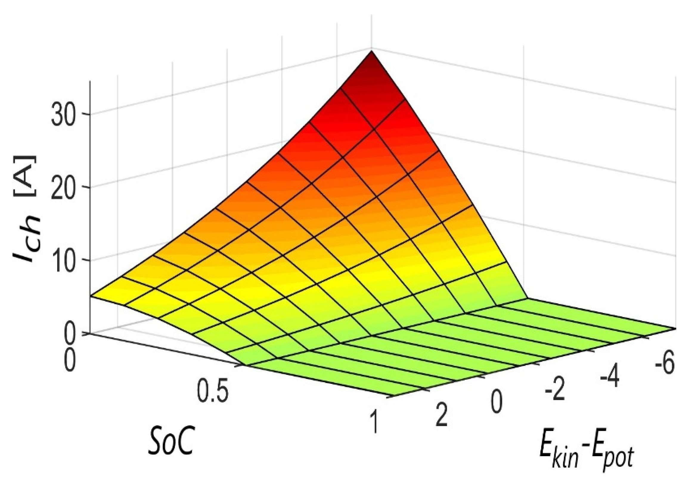
Figure 16 and
Figure 17 show the control surfaces that determine reference for the supercapacitor charging current from the power grid in order to obtain the minimum energy algorithm and the minimum gradient algorithm. It can be seen that for the first algorithm, the tendency is to charge from the grid as infrequently as possible, i.e., to use the energy of regenerative braking as much as possible. This behavior is logical, since the area in which the savings occur is irrelevant for the algorithm and what is important is how much energy is stored. Increasing the current limit of the supercapacitor further reduces the charge from the grid. For the second algorithm, on the other hand, it is more important that the energy of the supercapacitor is readily available to reduce the current peaks from the power grid, so that it is almost always necessary to recharge the supercapacitor. Increasing the current limit of the supercapacitor further increases the charge from the grid.
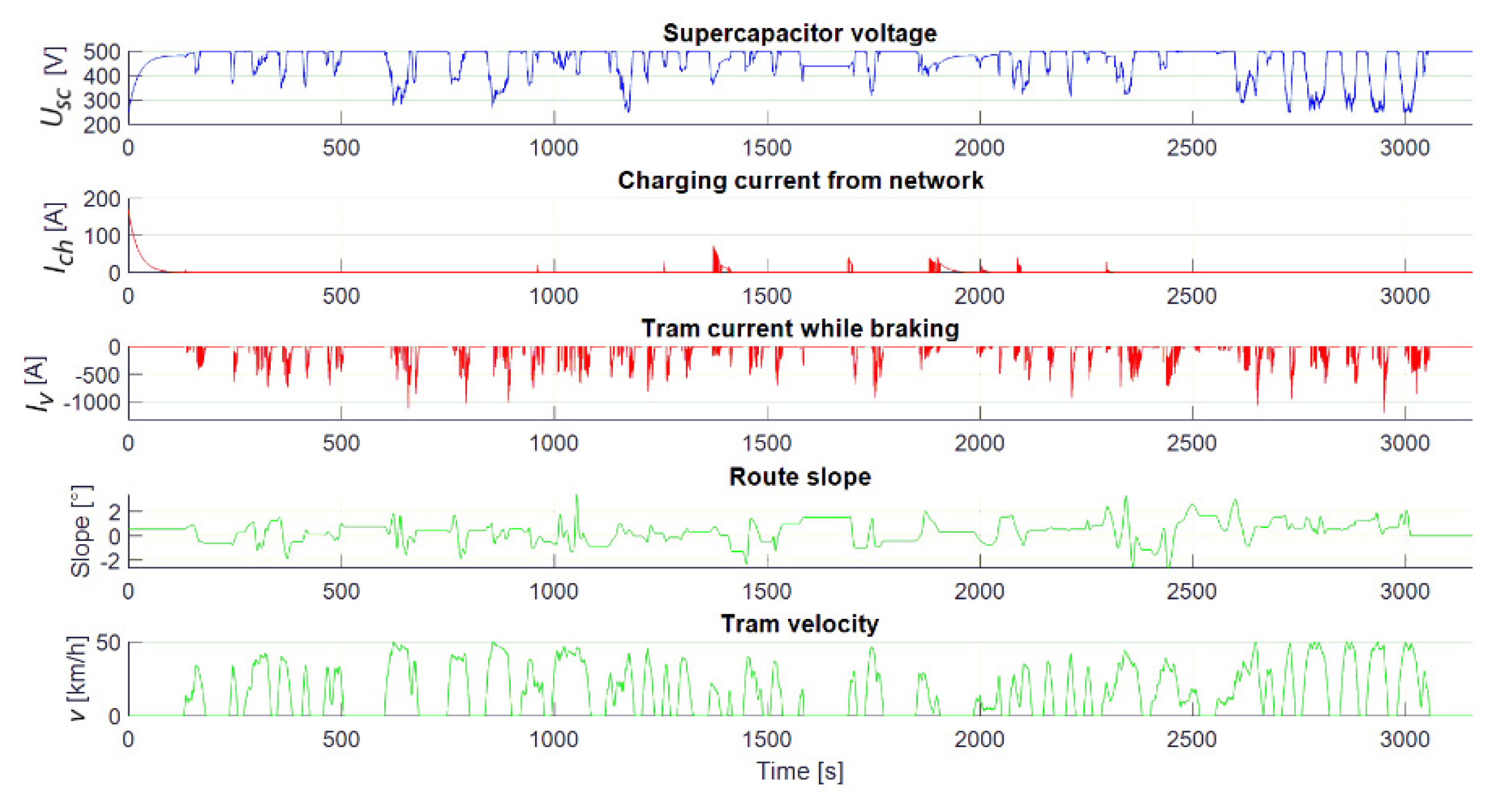
Figure 18 shows the voltage waveforms of the supercapacitor, the charging current from the grid, and the regenerative braking current according to the minimum energy algorithm, as well as the slope of the track and the speed of the tram. Looking at the speed profile, it is seen that it is a periodic acceleration and deceleration of the tram. Periods of rest on part of the track are tram stops. From
Figure 18, it can be seen that the supercapacitor is not charged by the grid during most of the track. Since the criterion is the minimum energy taken from the grid, this result was expected.
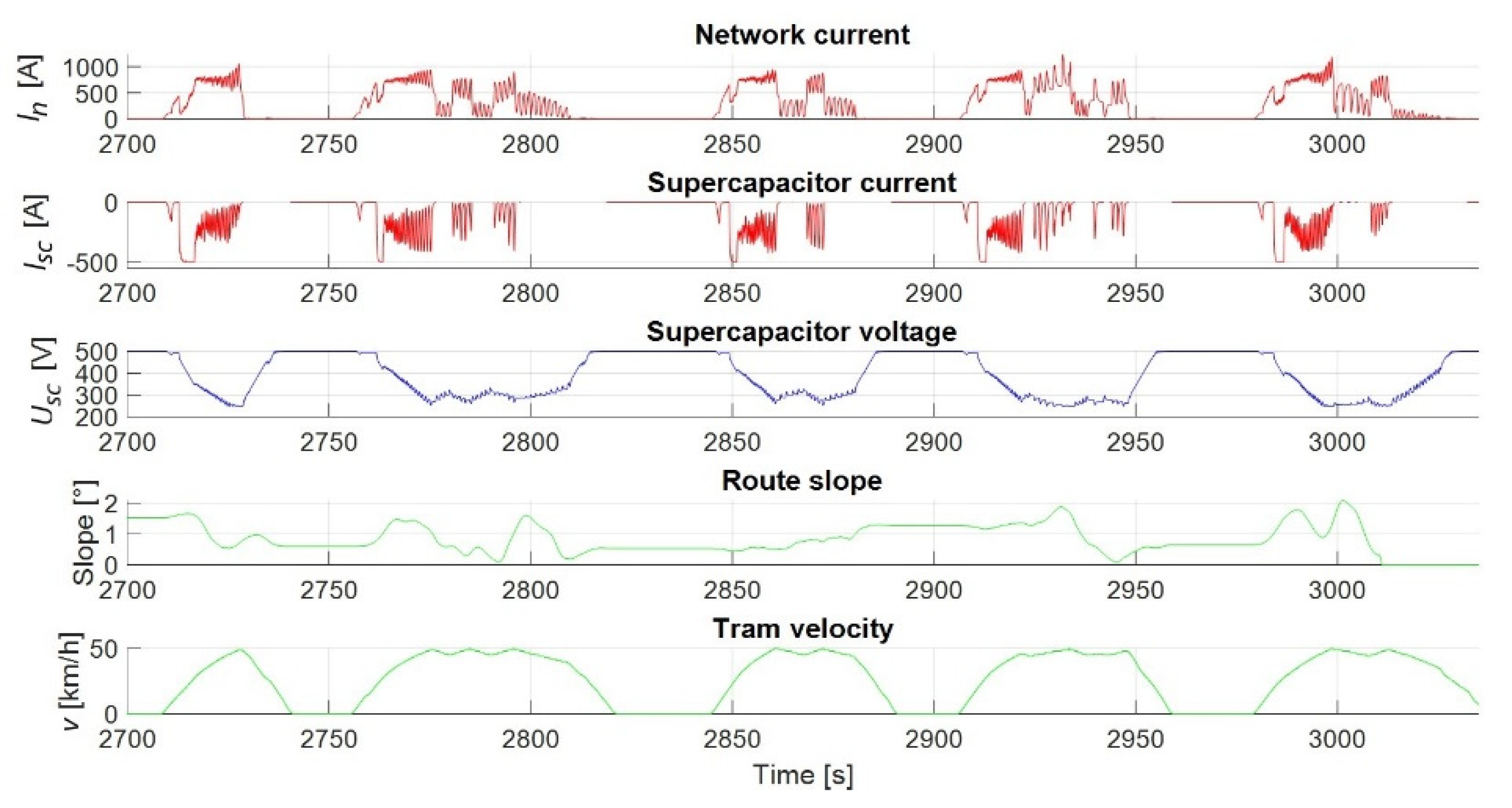
Figure 19 shows the voltage waveforms of the supercapacitor and the charging current from the grid and regenerative braking current according to the minimum network current gradient algorithm, as well as the slope of the track and the speed of the tram. It can be observed that in this case, the supercapacitor is charged more frequently from the grid to reduce the peak current values of the grid. Comparing the supercapacitor voltage waveforms with the minimum energy algorithm and the minimum gradient, it can be seen that in the minimum gradient algorithm, the voltage value is closer to the maximum state of charge, i.e., the average voltage value during the track is higher than in the minimum energy algorithm.
4.2.3. Supercapacitor Energy during Discharge
In this subsection, the energy of the supercapacitor during discharge is analyzed.
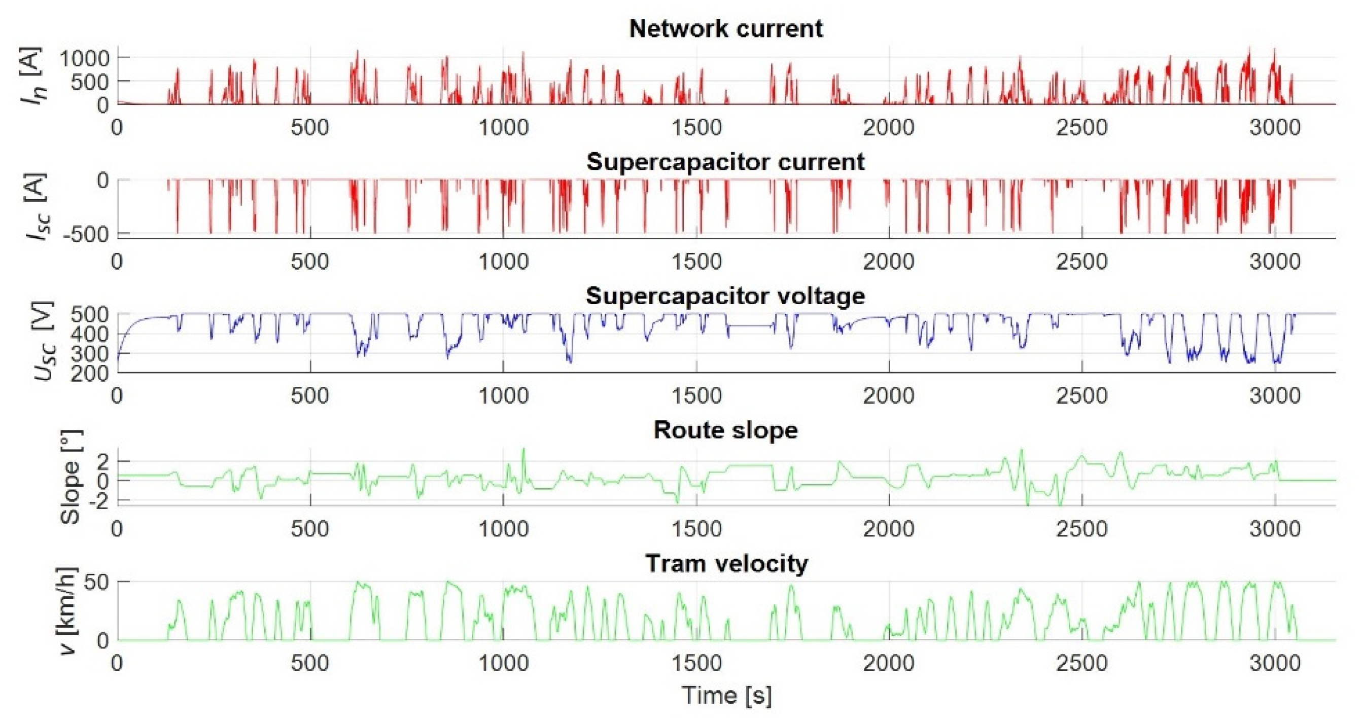
Figure 20 shows the profiles of the grid current, the current and voltage of the supercapacitor, the gradient of the track, and the speed of the tram for the parameters defined by the minimum energy criterion for line No. 14. The first and second graphs in
Figure 20 represent the total traction current, where a negative supercapacitor current indicates a discharge of the supercapacitor. From the voltage waveform, it can be seen that in the first half of the track, where the track is flat, the supercapacitor is involved to a lesser extent as a source of energy. Exceptions are instances like the one around 600 s into the simulation, where a constant acceleration towards the maximum speed is achieved on the part of the track with a positive gradient. Another example of a deeper discharge is at around 1100 s into the simulation. This is a classic example where the tram accelerates to about half of its maximum speed, maintains its speed for a while, and then continues to accelerate. However, in the part of the track after 2500 s, the supercapacitor is discharged to a minimum state of charge. From the graph of the slope of the track it can be seen that it is predominantly a positive slope, so a significant discharge is to be expected. This section represents the most critical part.
Figure 21 shows an enlarged view of this part of the track. It can also be seen from the voltage waveform that the supercapacitor reaches the minimum state of charge before the tram reaches maximum speed. Since the parameters of the control algorithm were determined for the minimum energy criterion, the supercapacitor releases the large amount of energy for acceleration at about half the acceleration time and there is no possibility to cover the peak current.
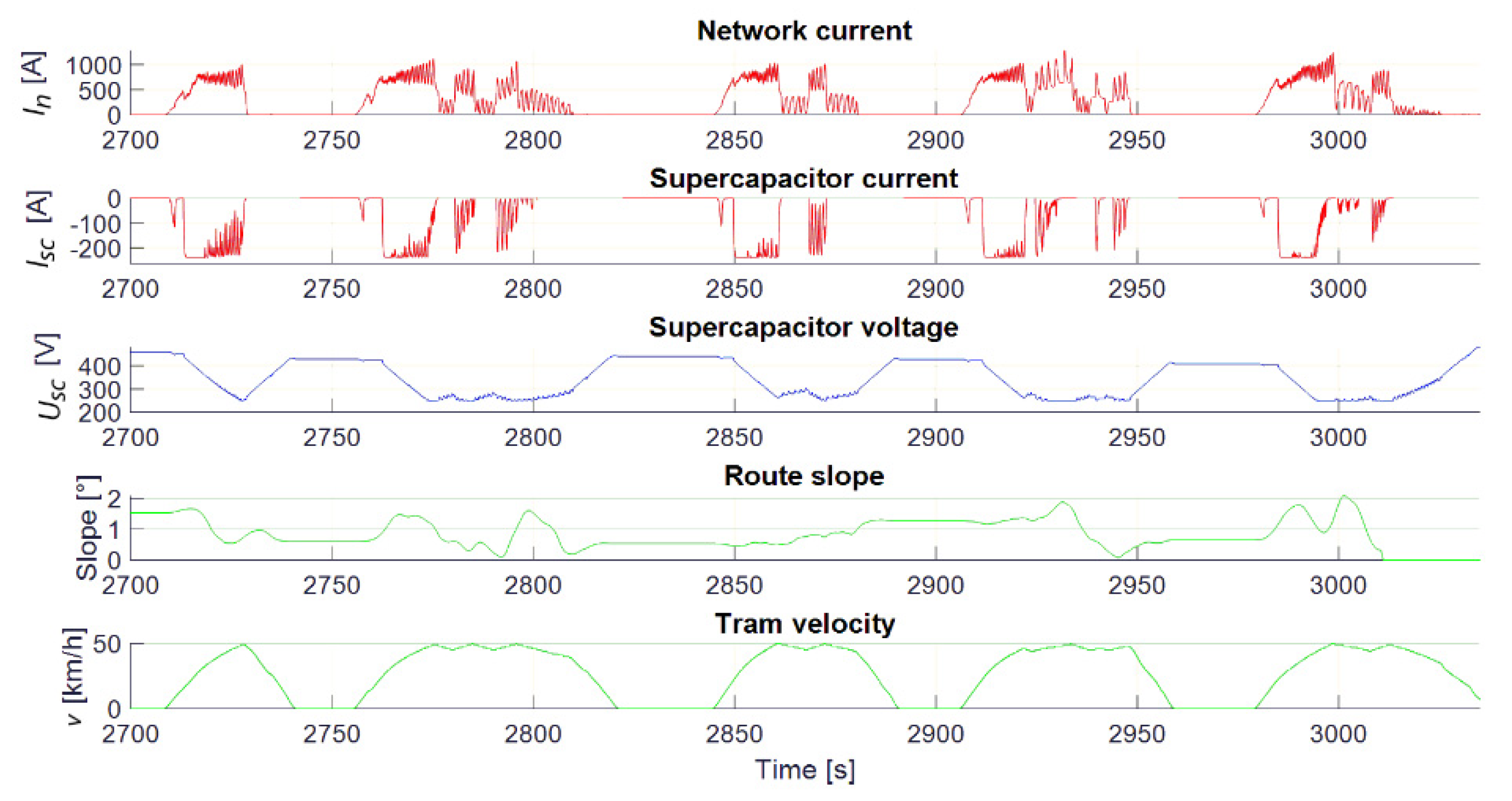
Figure 22 shows the case with the parameters determined according to the minimum gradient criterion. A large difference in the discharge of the supercapacitor module with respect to the minimum energy criterion can be seen. In this case, the supercapacitor never reaches the value of minimum state of charge. Moreover, on the critical part of the track, the peak values of the power grid current, were reduced.
Figure 23 shows an enlarged view of this section of the track. It can be seen that the supercapacitor does not reach the minimum state of charge in this case. This effect is achieved by the limited energy absorption from the supercapacitor at the beginning of the tram acceleration. At the very beginning, the supercapacitor is involved as an energy source. However, as the tram current increases, at one point the grid takes over the load. This moment represents a transition from the zone of low kinetic energy to the zone of medium kinetic energy. Only at the moment when the tram switches from the medium to the high kinetic energy zone, the supercapacitor is used as a source of the required energy.
Table 5 and
Table 6 show the energy saving data taken from the grid and the average value of the grid current for all cases. It can be seen that the minimum energy algorithm achieves greater energy saving compared to the minimum gradient algorithm. This is because the use of the supercapacitor energy affects the reduction of the energy taken from the grid and hence the reduction of the average value of the grid current. In the minimum gradient algorithm, due to the relatively high state of charge of the supercapacitor storage, the energy of regenerative braking is used less.
5. Conclusions
This paper presents an algorithm for storing and utilizing the energy of regenerative tram braking, which also takes into account the track elevation profile. The influence of the secondary energy source, i.e., supercapacitor storage, on the current-voltage relationships in the hybrid power system, which enables energy savings from the power grid and reduction of the power grid peak load, is analyzed. Prior to the analysis, simplified models of the rail vehicle, the power grid, and the supercapacitor were developed for the MATLAB/Simulink software package. The control algorithm is developed in order to control the energy flow in regenerative braking and storage system. The operation of the control algorithm was tested on two lines of Zagreb Electric Tram, line No. 14 in both directions and line no. 11, for two different criterion functions. Both criterion functions successfully reduced the maximum peak currents (up to 20%, depending on the selected line) and the total energy taken from the grid (up to 21%, depending on the selected line), by using regenerative braking energy. When the criterion of minimum energy taken from the grid was used, 2% to 6% higher energy savings and a lower mean value of the grid current were obtained compared to the second criterion. On the other hand, using the criterion of minimum sum of squares of the grid current gradient, the results show a reduction in the maximum peak currents (between 11% and 21%) and a significantly lower number of peaks above 1000 A (between 72% and 98%) compared to the second criterion. Compared to the minimum energy criterion, up to 20% higher savings are obtained. Increasing the current limit of the supercapacitor generally increased the energy savings and decreased the peak currents. Regarding the recharging of the supercapacitor with energy from the grid, it was shown that the choice of criterion function strongly influenced the shape of the charging area. The minimum energy criterion reduced the supercapacitor recharging from the grid. For the second criterion function, the charging of the supercapacitor from the grid was found to be a key factor in reducing the peak loads on the whole route. Depending on the specific route, the available voltage range of the supercapacitor is used to a greater or lesser extent. The developed algorithms allow significant energy saving in comparison to algorithm without using regenerative breaking energy. In addition, the algorithms show significant improvement in behavior on sloped tracks, in comparison with the cited regenerative braking algorithms. It is not enough just to store the energy of regenerative braking and use it during the next acceleration. The key aspect is to store as much energy as possible and use it to compensate the adverse effects on the power supply network generated by the rail vehicle, such as accelerating a tram uphill. In this paper, those are the moments when a tram accelerates to above 25 km/h, while traveling uphill. Future development of the algorithm would include HIL simulations, as well as drive tests, in which other real-world factors could be taken into account. Further research will allow the control algorithm to be modified in order to allow even greater power grid load reduction, extend the life of the supercapacitor, and improve the performance of the rail vehicle.


