Article

An Open Circuit Voltage Model Fusion Method for State of Charge Estimation of Lithium-Ion Batteries

1
School of Automotive Engineering, Harbin Institute of Technology, Weihai 264209, China
2
National Engineering Laboratory for Electric Vehicles, School of Mechanical Engineering, Beijing Institute of Technology, Beijing 100081, China
*
Author to whom correspondence should be addressed.
Energies 2021, 14(7), 1797; https://doi.org/10.3390/en14071797
Submission received: 6 February 2021 / Revised: 7 March 2021 / Accepted: 18 March 2021 / Published: 24 March 2021

Abstract

:
The mapping between open circuit voltage (OCV) and state of charge (SOC) is critical to the lithium-ion battery management system (BMS) for electric vehicles. In order to solve the poor accuracy in the local SOC range of most OCV models, an OCV model fusion method for SOC estimation is proposed. According to the characteristics of the experimental OCV–SOC curve, the method divides SOC interval (0, 100%) into several sub-intervals, and respectively fits the OCV curve segments in each sub-interval to obtain a corresponding number of OCV sub-models with local high precision. After that, the OCV sub-models are fused through the continuous weight function to obtain fusional OCV model. Regarding the OCV curve obtained from low-current OCV test as the criterion, the fusional OCV models of LiNiMnCoO2 (NMC) and LiFePO4 (LFP) are compared separately with the conventional OCV models. The comparison shows great fitting accuracy of the fusional OCV model. Furthermore, the adaptive cubature Kalman filter (ACKF) is utilized to estimate SOC and capacity under a dynamic stress test (DST) at different temperatures. The experimental results show that the fusional OCV model can effectively track the performance of the OCV–SOC curve model.

1. Introduction

In response to the various policies of sustainable development, the development of electric vehicles (EVs) with batteries as the main power source has become the theme of the automotive industry. Because of numerous appealing characteristics, lithium-ion batteries (LiBs) have been an indispensable part of EVs [1]. As a significant indicator, the state of charge (SOC) dominates the range anxiety of drivers. Precise and reliable SOC estimation allows battery management system (BMS) to protect the battery, prevent overcharge/over-discharge, extend the battery life, and make reasonable control strategies to save energy [2,3]. Therefore, SOC estimation always attracts the attention of academia and the industrial community.
Various approaches of SOC estimation have been developed [4,5,6,7]. The classical approach to estimate SOC is the ampere-hour integral method which directly originates from the definition of the SOC. The precision of ampere-hour integral method is seriously limited by the initial SOC error, sensor error and battery aging [8]. Model-based methods have been extensively used due to their self-correcting merits. The essence of model-based methods is the mapping between SOC and other battery parameters like impedance spectroscopy and open circuit voltage (OCV). The Kalman filter is commonly used to estimate SOC in various model-based methods with the bearable amount of calculation cost and the supply of state uncertainty. The Kalman filter algorithm family includes the classical Kalman filter, extended Kalman filter (EKF) [9,10], unscented Kalman filter (UKF) [11], cubature Kalman filter (CKF) [12] and all the extensive form of Kalman filter. EKF needs to solve the Jacobi matrix, which limited its computation speed and remains just 1 order Taylor expansion precision [13]. UKF needs to set reasonable noise parameter and sigma point configuration parameter, which is dependent on specific battery working conditions. CKF generates the cubature points to approximate the state transfer function. With fewer parameters that need to be adjusted and minimal calculation costs, CKF remains in 3 order Taylor expansion precision. Therefore, CKF is generally more practical than EKF and UKF. In order to solve the possible divergence of the filter, the adaptive extended Kalman filter (AEKF) and adaptive unscented Kalman filter (AUKF) have been studied [14,15,16]. In this paper, the adaptive cubature Kalman filter (ACKF) is introduced to estimate SOC.
For the model-based method, the precision of the OCV–SOC function model (OCV model) which reflects the mapping between SOC and OCV seriously determines the performance of SOC estimation. The incremental OCV test and the low-current OCV test are usual experiments to obtain experimental OCV–SOC characteristic curve (OCV curve) [17,18]. In the same time-consuming condition, the incremental method is slightly suitable for specific battery material system at a certain temperature [17]. However, the low-current OCV test provides intact OCV–SOC data points (OCV points), and the measured voltage can maintain close-to-equilibrium status if the current rate is extremely small [19]. Therefore, the OCV curves obtained by the low-current OCV test are more suitbale used as reference models (OCV curve models) for various OCV models.
OCV curve presents distinct characteristic with the change of battery material system it belongs and is influenced by ambient temperature, aging status and current rate [20]. OCV points obtained from OCV test can be sampled reasonably as control points to fit OCV curve. Lots of OCV function models have been proposed to express OCV curve [8]. The polynomial function, power function, logarithm and exponent are alternative choices to constitute the OCV model [21,22,23,24,25]. Among these functions, polynomial functions were commonly used to fit the OCV curve. By comparing five OCV models, Hu et al. [26] concluded that the sixth-order polynomial function was considered as the most accurate OCV model among them. In practice, most OCV models were adopted to fit incomplete OCV curve whose SOC range is between 10% and 90%. By setting cut-off voltage, the SOC range is commonly regarded as nominal 0–100% to ensure safety. So, the battery capacity is cut down by the control of the BMS, and not fully utilized. If the accuracy in the marginal region of the OCV model can be improved as much as possible, it will be helpful for BMS to further extend the cut-off voltage and increase the available battery capacity. Furthermore, establishing OCV models which satisfy high fidelity in the full SOC range is worth studying.
In order to solve the aforementioned problems, this paper attempts to make the following contributions:
  • An OCV model fusion method is proposed to obtain fusional OCV model which may match the characteristic of OCV curve in complete SOC range. The OCV model fusion method is applied for a LiNiMnCoO2 (NMC) battery and a LiFePO4 (LFP) battery. OCV fitting curves with high precision are obtained at temperature of 10 °C, 25 °C and 40 °C, respectively.
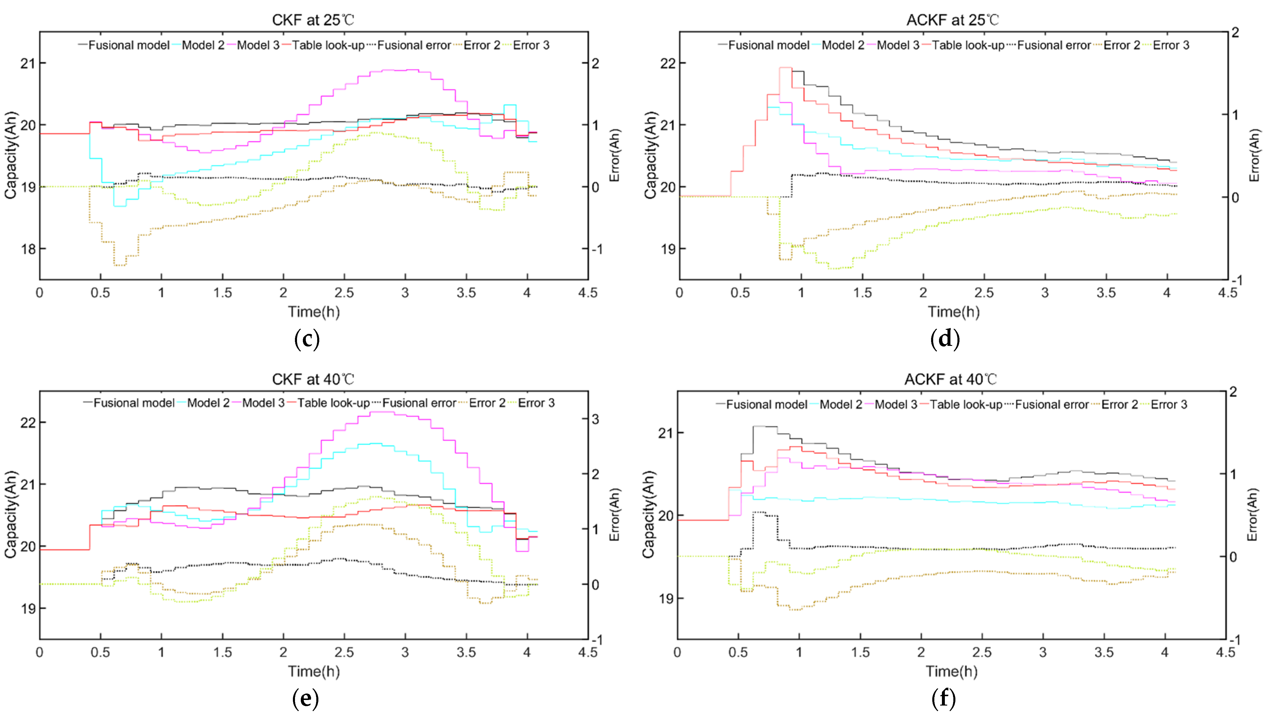
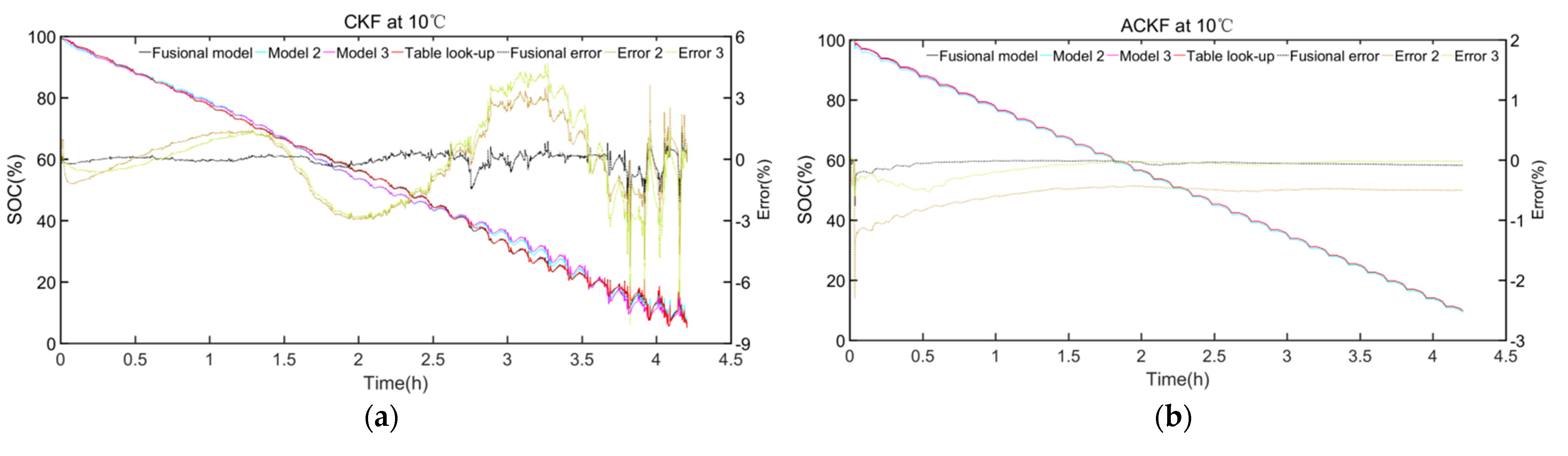
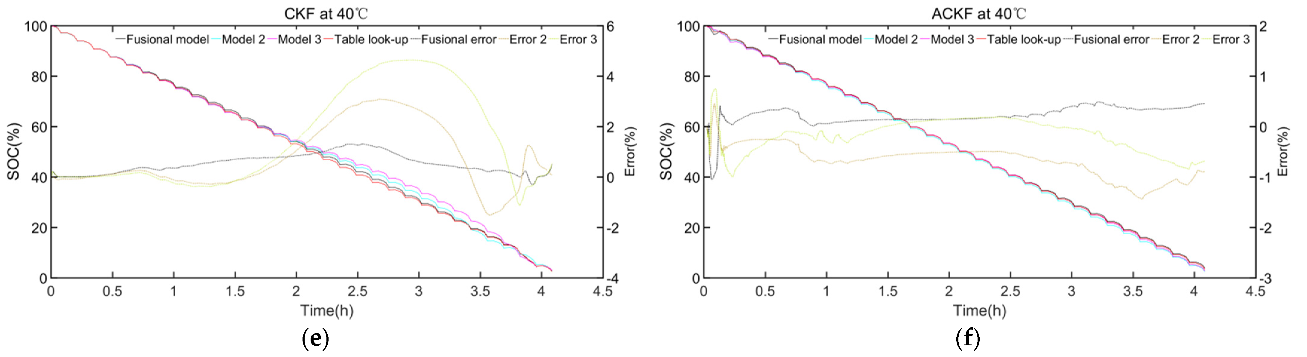
  • CKF and ACKF are utilized to estimate SOC and capacity, and the effect of the fusional OCV model on SOC and capacity estimation is evaluated by comparing with the OCV curve model. Besides, the adaptability of the ACKF algorithm for OCV model errors is verified.
Notably, this paper is concerned with how to obtain the OCV model with high fidelity based on limited but persuasive control points obtained from an experimental test.
The rest of this paper is organized as follows. Section 2 presents the battery model and OCV model fusion method. Section 3 introduces the ACKF and capacity estimation algorithm. Section 4 presents the experimental validation. Finally, conclusions are given in Section 5.

2. Battery Modeling and Open Circuit Voltage (OCV) Curve Fusion Method

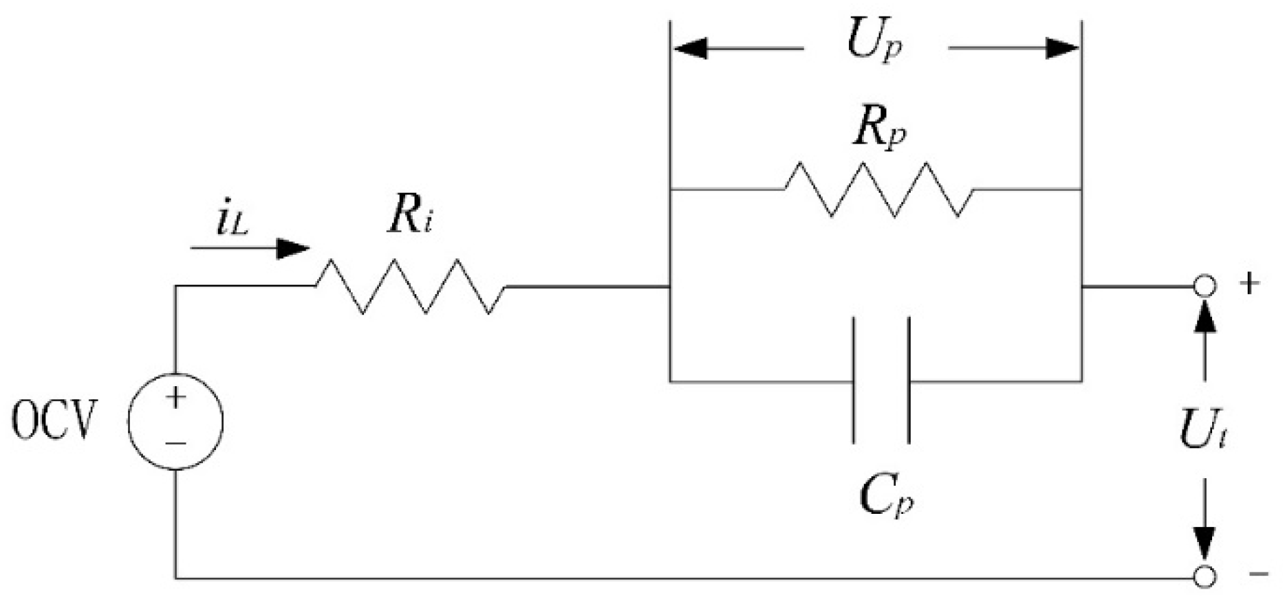
2.1. Battery Modelling

Battery models, the basis of battery algorithms, mainly include electrochemical mechanism models [27] and equivalent circuit models (ECMs) [28]. The electrochemical mechanism models are highly accurate but limited by unsustainable computation load. The ECMs describe dynamic characteristic and operation mechanism of batteries by using circuit network which comprises traditional resistance, capacitor, and constant voltage source. An resistor-capacitor (RC) network is commonly used to characterize the dynamic features of batteries. Among various ECMs, the first-order RC ECM as shown in Figure 1, also called the Thevenin model, shows the best balance between complexity and accuracy [29,30].
OCV denotes the terminal voltage which has a non-linear relationship with SOC; iL denotes the current of the battery; Ri denotes the internal resistance, and characterizes the contact resistance among battery electrode material, electrolyte, diaphragm resistance and various parts; Rp denotes polarization resistance and Cp denotes polarization capacitance, the parallel connection of Cp and Rp reveals the dynamic characteristics of the battery; Ut denotes the terminal voltage; Up denotes the potential difference of the RC network which is called polarization voltage.
The mathematical expression between Ut and iL is:
U t = O C V U p i L R i
The mathematical expression between Up and iL is:
U ˙ p = 1 C p R p U p + 1 C p i L
After discretizing the above equation, following equation is summarized as:
{ U p , k = U p , k 1 exp ( Δ t R p C p ) + i L , k 1 R p ( 1 e x p ( Δ t R p C p ) ) U t , k = O C V k U p , k R 0 i L , k 1
where the subscript k denotes the sampling step, Δt denotes the step size. OCVk is a nonlinear function of SOC. By calculating Equation (4), SOC is obtained.
SOC k = SOC k 1 η i Δ t C a i L , k
where ƞi denotes the coulombic efficiency of cell [31], Ca denotes current maximum available capacity which is directly relevant to battery aging and ambient temperature et al., so it is not fixed like nominal capacity. ƞi is generally defaulted as 1.
The terminal voltage Ut and the current iL in the Thevenin model can be measured by the voltage sensor and the current sensor respectively. In the meanwhile, the model parameters Ri, Rp, Cp and non-linear function OCVk have to be determined so that subsequent battery algorithm can be sustained. Because parameters are seriously influenced by the variable factors like battery temperature, aging status, charge or discharge current etc., recursive least squares method with forgetting factor (FFRLS) is utilized to identify parameters Ri, Rp, Cp in real time [32].

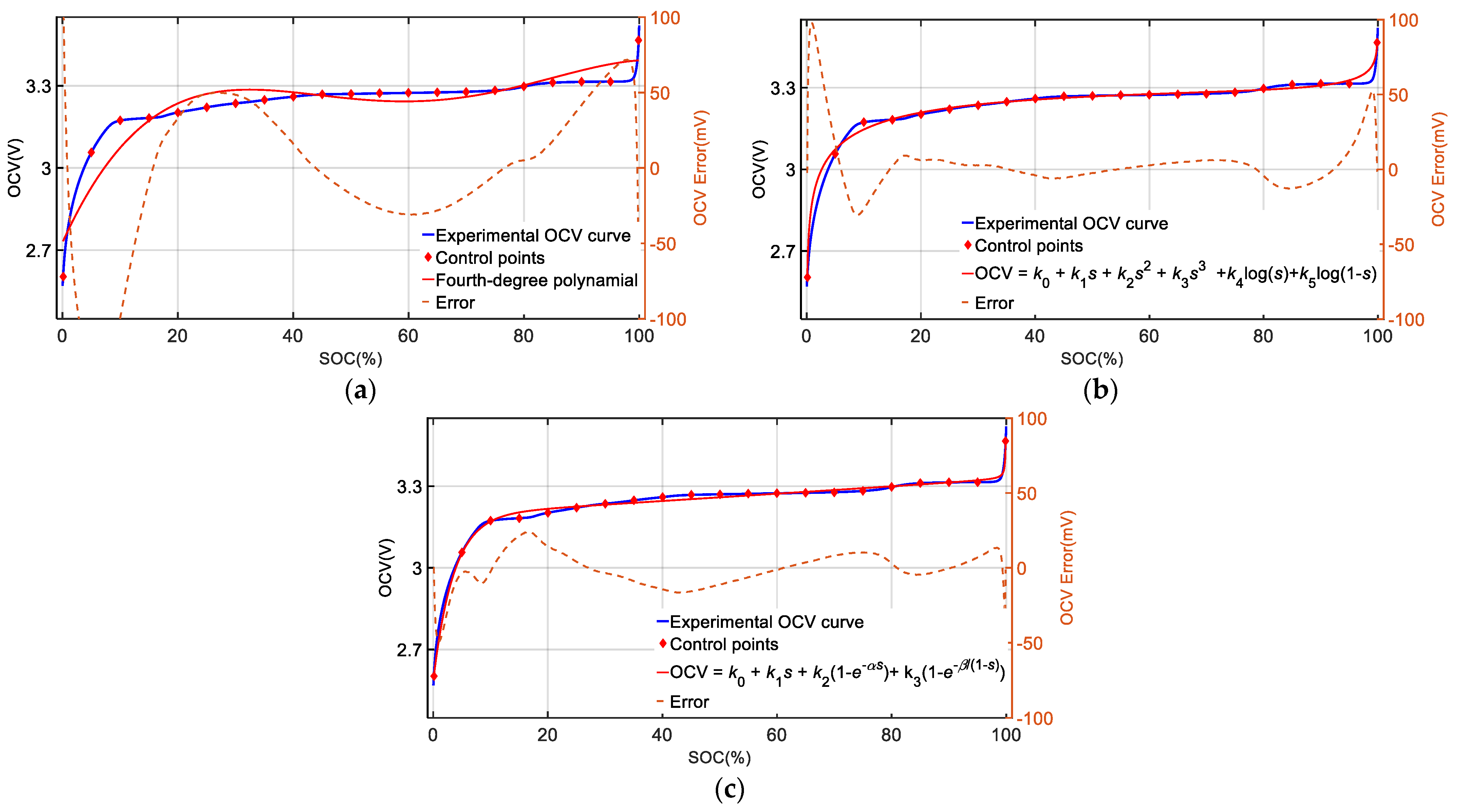
2.2. OCV Model Fusion Method

The mapping between OCV and SOC is a basic part of battery modeling. During the process of OCV model selection, the non-linearity of OCV curve brings out the toughest part. Based on the control points obtained from the OCV test, the coefficients of the OCV model can be solved after carrying out the curve fitting algorithm. The curves presented by the solved OCV models can be named as OCV fitting curves. Reasonable selection of the OCV model can maximize experiment effect as much as possible. From the perspective of structure, the components of OCV models basically include generalized polynomial, logarithm, exponent and power function. The polynomial functions satisfy the needs of general condition, but perform poorly in the local SOC range as shown in Figure 2a. Besides, polynomial functions may cause under fitting or overfitting if the number of control points do not match the degree of polynomials. The OCV model which consists of reasonable combination of polynomial, logarithm, exponent or power function may perform well in the global SOC range. However, it is still inevitable that the precision of OCV model in the local SOC range declines seriously, as shown in Figure 2b,c.
With further thinking about problems above, the reasons why it is difficult to perfectly fit the complete OCV curves can be summarized:
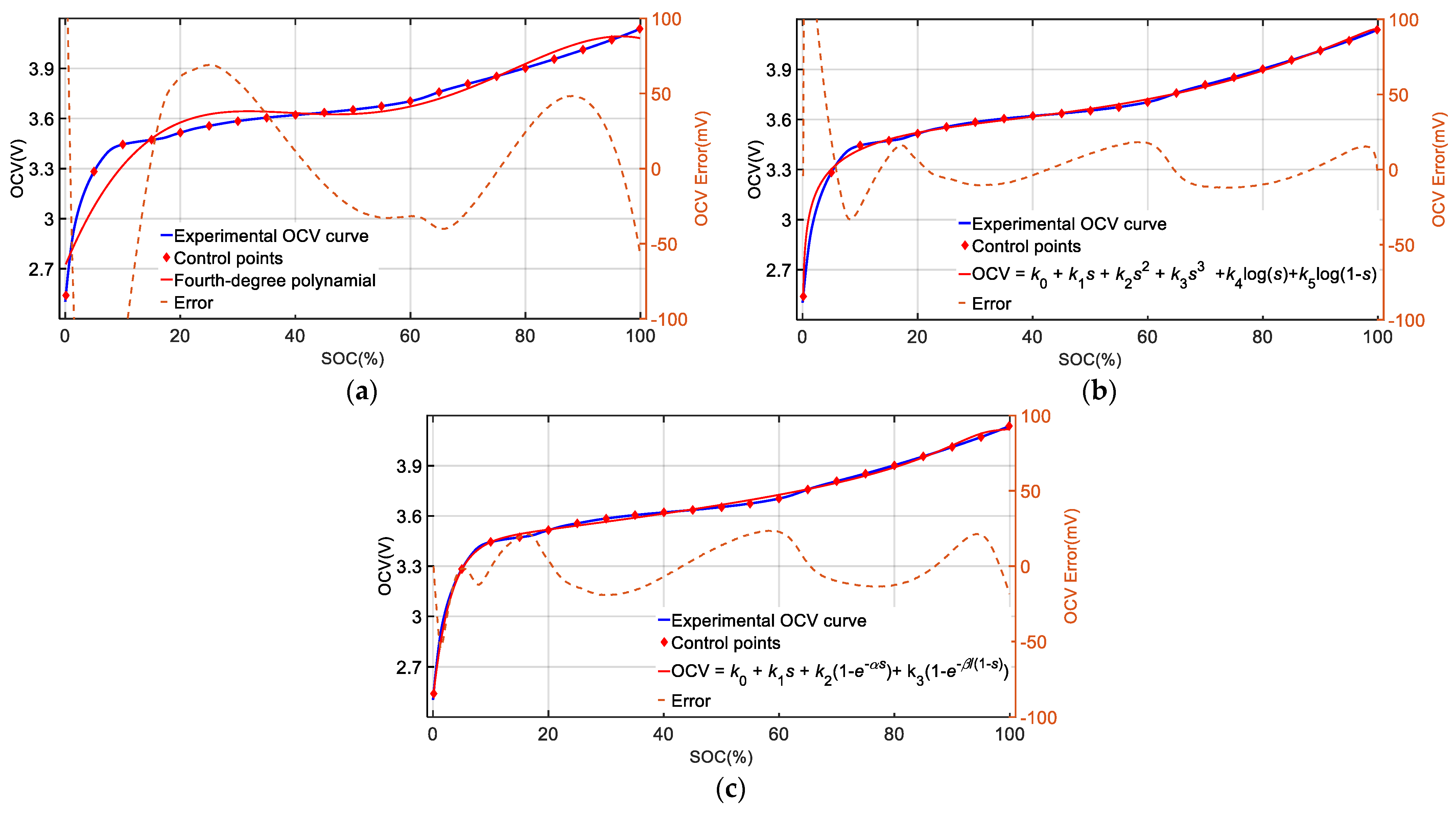
  • From the perspective of battery characteristics, the marginal region of some OCV curves may be polarized, and the changing trend of the OCV curves may be transformed within a small SOC range. It is difficult for the OCV model to fully take into account the characteristics of the OCV curve.
  • From the perspective of practical application, some algorithms are sensitive to the error of OCV fitting curve. For example, the OCV curve of a LFP battery may have several large flat regions. If SOC is inferred from the OCV based on OCV fitting curve which is stored in a table, the error of OCV will lead to larger error of the SOC due to the deviation of flat regions. Therefore, the requirement for the OCV model’s accuracy is strengthened.
The problems caused by former reason is the focus of this paper. Predictably, if a single OCV curve segment with stable changing trend is extracted for fitting, then a high-precision OCV fitting curve segment can be obtained correspondingly. However, it is a question of combining all these OCV fitting curve segments. In order to obtain OCV fitting curve which can maintain high fidelity in the local SOC range as much as possible, an OCV model fusion method is proposed. Figure 3 demonstrates the flowchart of the OCV model fusion method which fits an OCV curve of NMC battery.
For different types of battery, the general steps are as follows:
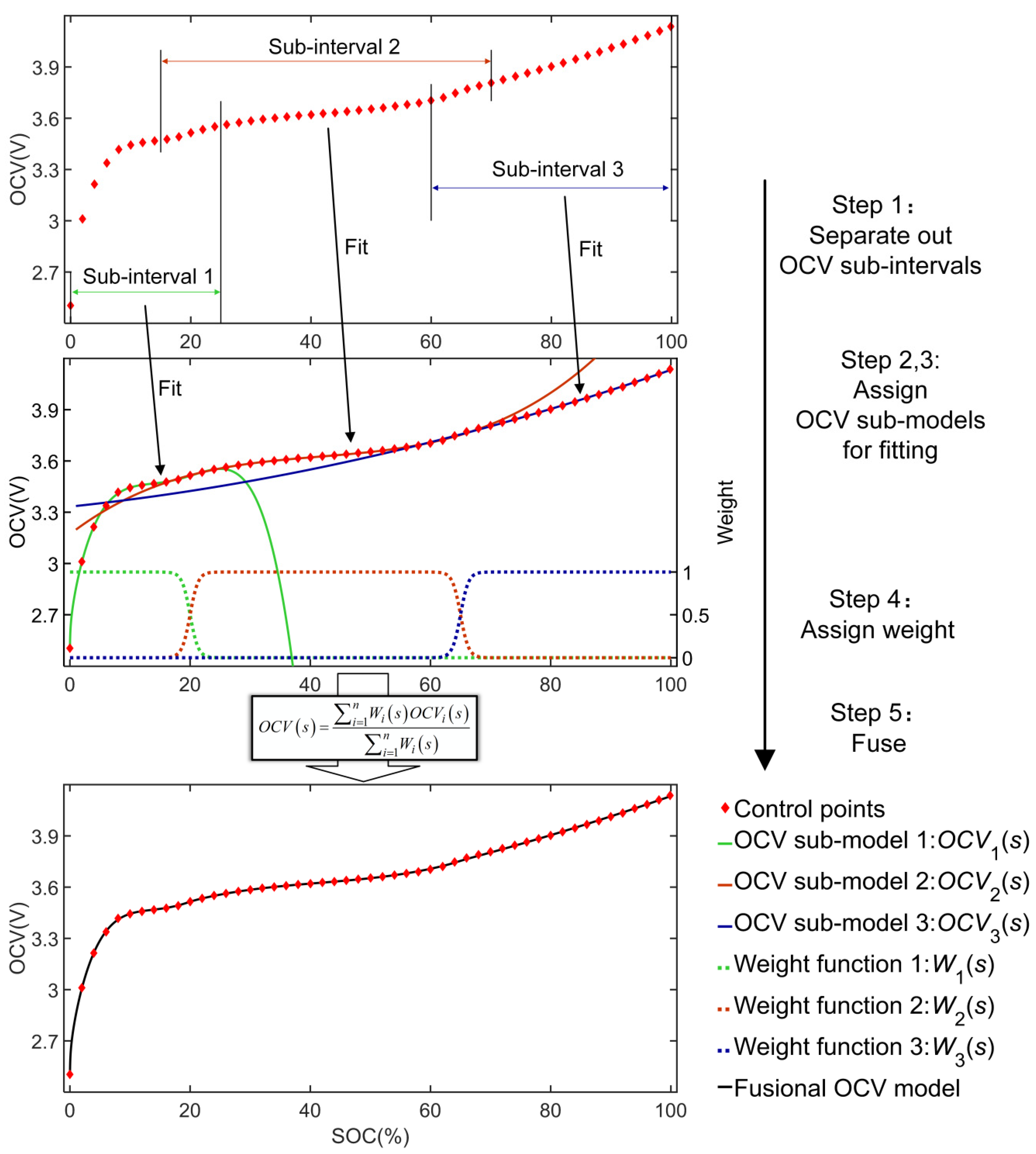
  • Separate out OCV sub-intervals: according to the characteristics of OCV curve, the global SOC interval (0, 100%) can be divided into several local sub-intervals. In order to ensure the smoothness of fusional curve, each sub-interval exists overlap with neighboring sub-intervals.
  • Assign OCV sub-models: according to the characteristics of the OCV curve in the local SOC sub-interval, each sub-interval corresponds to a specific OCV sub-model.
  • Curve segment fitting: according to practical conditions, collecting the control points in each sub-interval. After fitting, the OCV fitting curve segments of all sub-models are obtained.
  • Assign weight: different global weight functions are assigned to corresponding OCV sub-models. The function should convert weight from high to low continually when the SOC gradually away from sub-interval in the overlapped region. Logistic function is suitable for defining conversion above.
  • Fuse: according to weight functions, all OCV sub-models can fuse into a fusional OCV model. The final OCV fitting curve can be expressed by using equation as follows:
    O C V ( s ) = i = 1 n W i ( s ) O C V i ( s ) i = 1 n W i ( s )
    where s denotes SOC, OCVi(s) denotes the OCV value of sub-model i at s, Wi(s) denotes the corresponding weight at s. The final fusional OCV model can be directly used for subsequent algorithms.
Theoretically, the proposed OCV model fusion method is universal for any type of battery as long as the OCV model can be used to fit the OCV curve. As representative commercial lithium-ion batteries, the LFP battery and NMC battery are used to verify the effectiveness of the proposed fusion method. Detailed application of the OCV fusion method in the two batteries is presented.

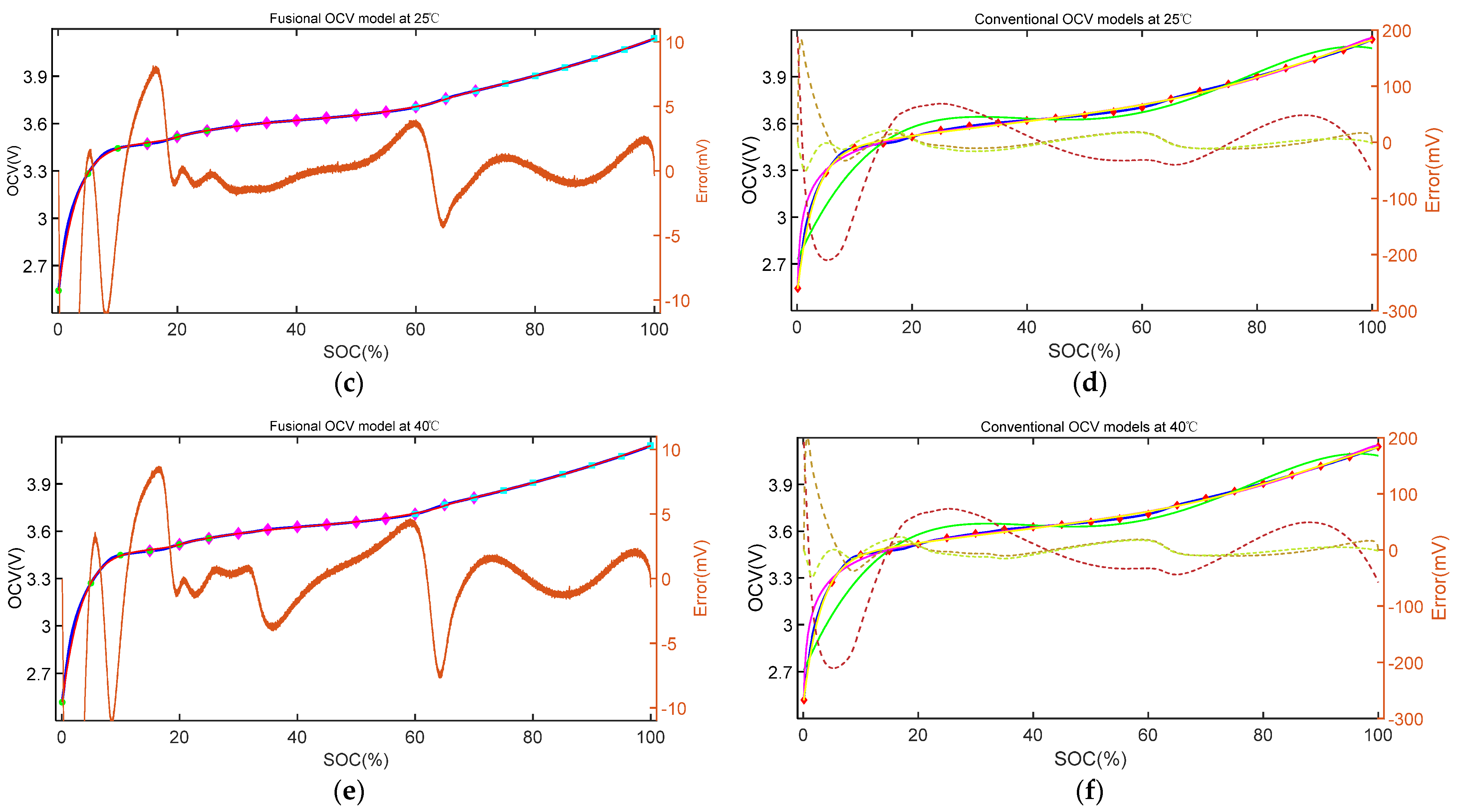
2.2.1. Method for LiNiMnCoO2 (NMC) Battery Cell

An OCV curve of NMC battery with changing rate of OCV over SOC is presented in Figure 4. Due to the discrete form of OCV curve, the changing rate of OCV is approximately calculated through the following equation:
O C V ( s ) O C V ( s + 0.1 % ) O C V ( s 0.1 % ) 0.2 %
By analyzing the OCV curve of NMC battery, the following characteristics can be summarized:
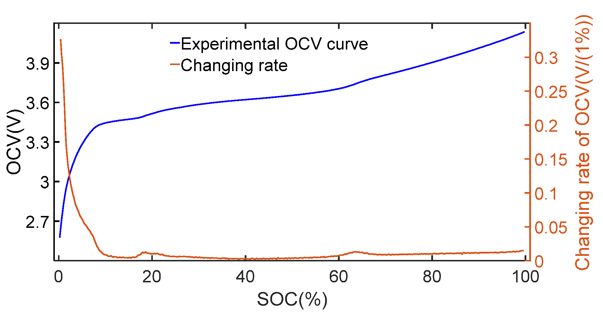
  • The OCV curve is clearly monotonous, and OCV changes dramatically when SOC drops to 0%.
  • By approximately calculating the changing rate of the OCV with SOC, it is obvious that the changing rate of OCV curve has bumps around 20% SOC and 65% SOC.
The OCV models in Figure 2 are adopted to fit global OCV curve, and the results show that the accuracy fluctuates when the SOC is around 20% and 65%. Intuitively, it is easy to obtain an accurate OCV sub-model by fitting an OCV curve segment whose approximate range of SOC is (20%, 65%). By setting interval (15%, 25%) and interval (60, 70%) as conversion region, the OCV curve is divided into three parts. The corresponding sub-intervals are (0, 25%), (15%, 70%) and (60%, 100%).
In order to verify the effect of fusion method, the OCV models in Figure 2 are alternative choice of OCV sub-models. Due to the strongly non-linear variation of the OCV curve when SOC drops to 0%, the exponent, logarithm and power function are alternative choices of OCV sub-model for sub-interval (0, 25%). The OCV model in Figure 2c shows the best accuracy in sub-interval (0, 25%), so it is adopted. The variation of the OCV curve is nearly linear in sub-intervals (15%, 70%) and (60%, 100%), so corresponding sub-models with polynomial would be adequate for fitting. OCV sub-models adopted for a NMC battery are presented in Table 1.
After collecting enough control points in three sub-intervals respectively, the fitting results can be obtained. Weight function of each sub-interval is defined as:
{ W N M C , 1 ( s ) = 1 1 + e x p ( r ( s 0.2 ) ) W N M C , 2 ( s ) = { 1 1 + e x p ( r ( s 0.2 ) ) ,   s 0.425 1 1 + e x p ( r ( s 0.65 ) ) ,   s > 0.425 W N M C , 3 ( s ) = 1 1 + e x p ( r ( s 0.65 ) )
where r denotes the shape parameter which determines the degree of weight conversion. In this paper, r is configured as 150.

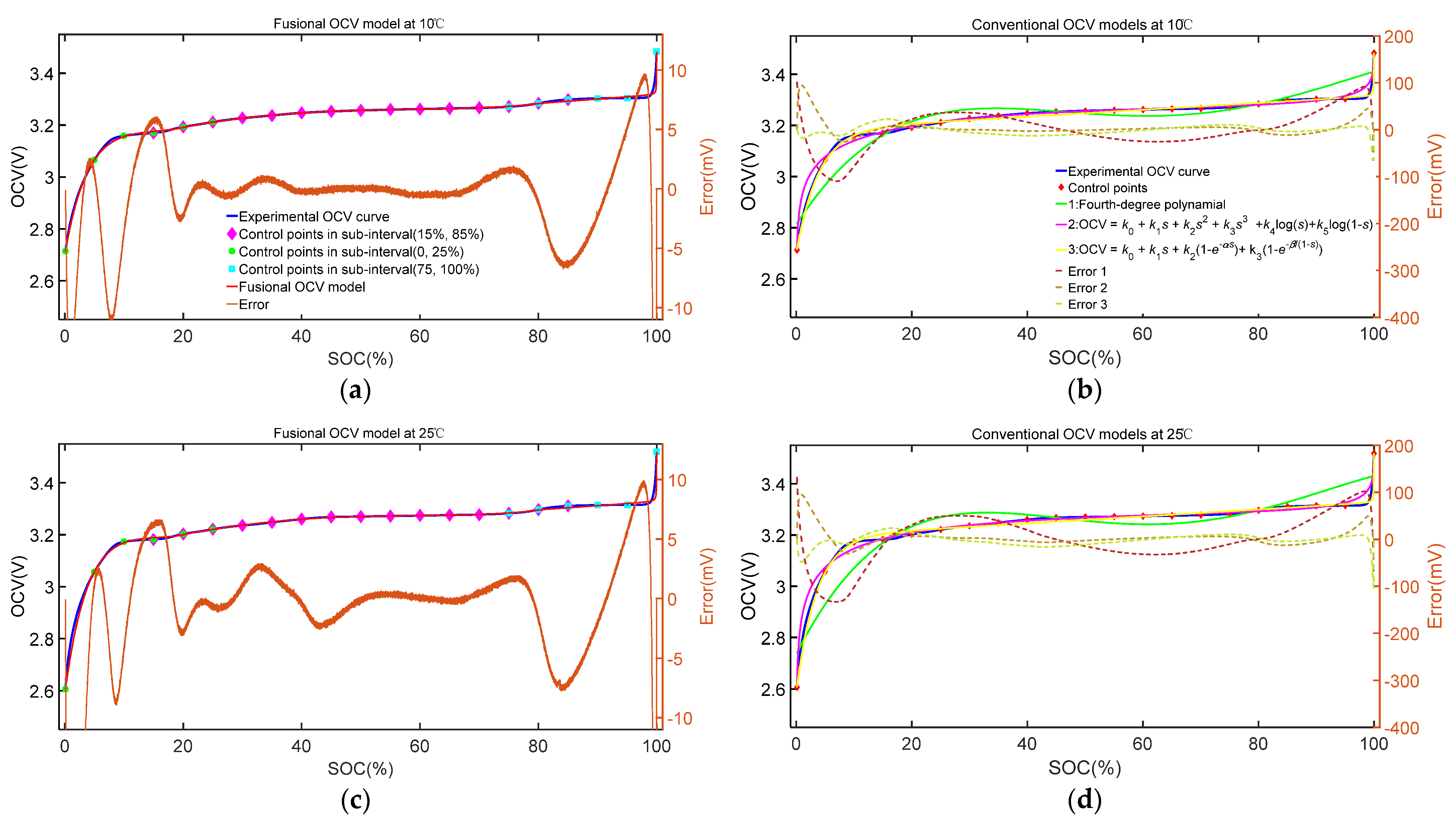
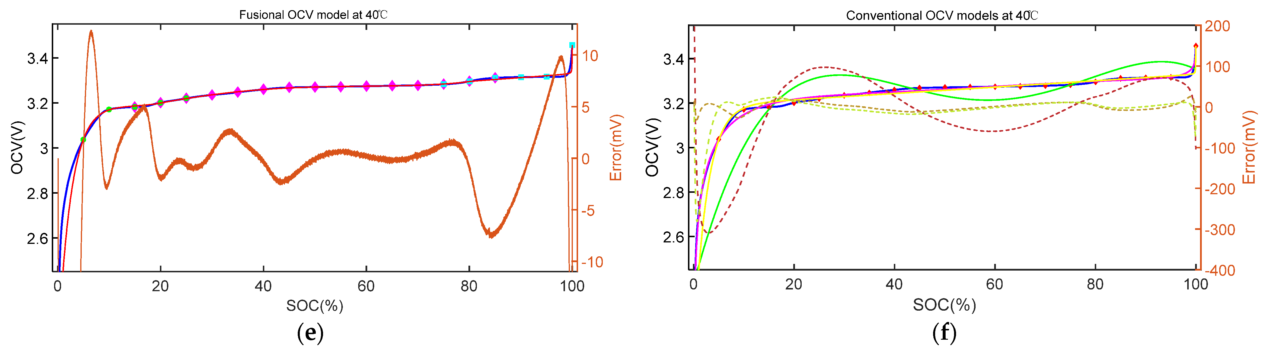
2.2.2. Method for LiFePO4 (LFP) Battery Cell

An OCV curve of a LFP battery with changing rate of OCV over SOC is presented in Figure 5. Similarly, following the OCV characteristics of LFP battery can be summarized:
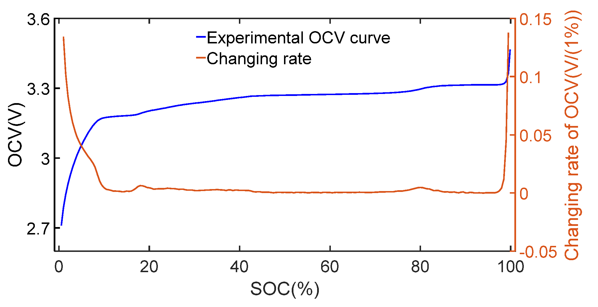
  • The OCV curve is monotonous, and the OCV changes dramatically when SOC drops to 0% and rises to 100%. Moreover, the OCV curve has flat regions where the changing rate of OCV is close to zero.
  • By approximately calculating the changing rate of OCV with SOC, it is obvious that the changing rate of the OCV curve has bumps around 20% SOC and 80% SOC.
Different OCV models in Figure 6 are adopted to fit OCV curve, and the results shows that accuracy fluctuates when SOC is around 10%, 20% and 80%. By setting interval (15%, 25%) and interval (75%, 85%) as the conversion region, OCV curve is divided into three parts. The corresponding sub-intervals are (0, 25%), (15%, 85%) and (75%, 100%). The OCV model in Figure 6c is adaptable to the strongly non-linearity of the LFP battery, which makes it become the OCV sub-model of sub-intervals (0%, 25%) and (75%, 100%). The OCV model in Figure 6b retains great precision in sub-interval (15%, 85%). The OCV sub-models adopted for the LFP battery are presented in Table 2.
After collecting enough control points in three sub-intervals respectively, the fitting results can be obtained. The weight function of each sub-interval is defined as:
{ W 1 ( s ) = 1 1 + e x p ( r ( s 0.2 ) ) W 2 ( s ) = { 1 1 + e x p ( r ( s 0.2 ) ) ,   s 0.5 1 1 + e x p ( r ( s 0.8 ) ) ,   s > 0.5 W 3 ( s ) = 1 1 + e x p ( r ( s 0.8 ) )
So far, the fusional OCV models of both batteries can be obtained by Equation (5) respectively. There are few points that need to be discussed:
  • Although the fusional results are deduced from two examples, the steps of fusion method are generalized.
  • According to practical condition, parameters like sub-intervals, sub-models and weight function can be explored freely.
  • It is not suitable to select a sub-interval with too short a length, otherwise the number of control points need to be increased.

3. State of Charge (SOC) and Capacity Estimation Algorithm

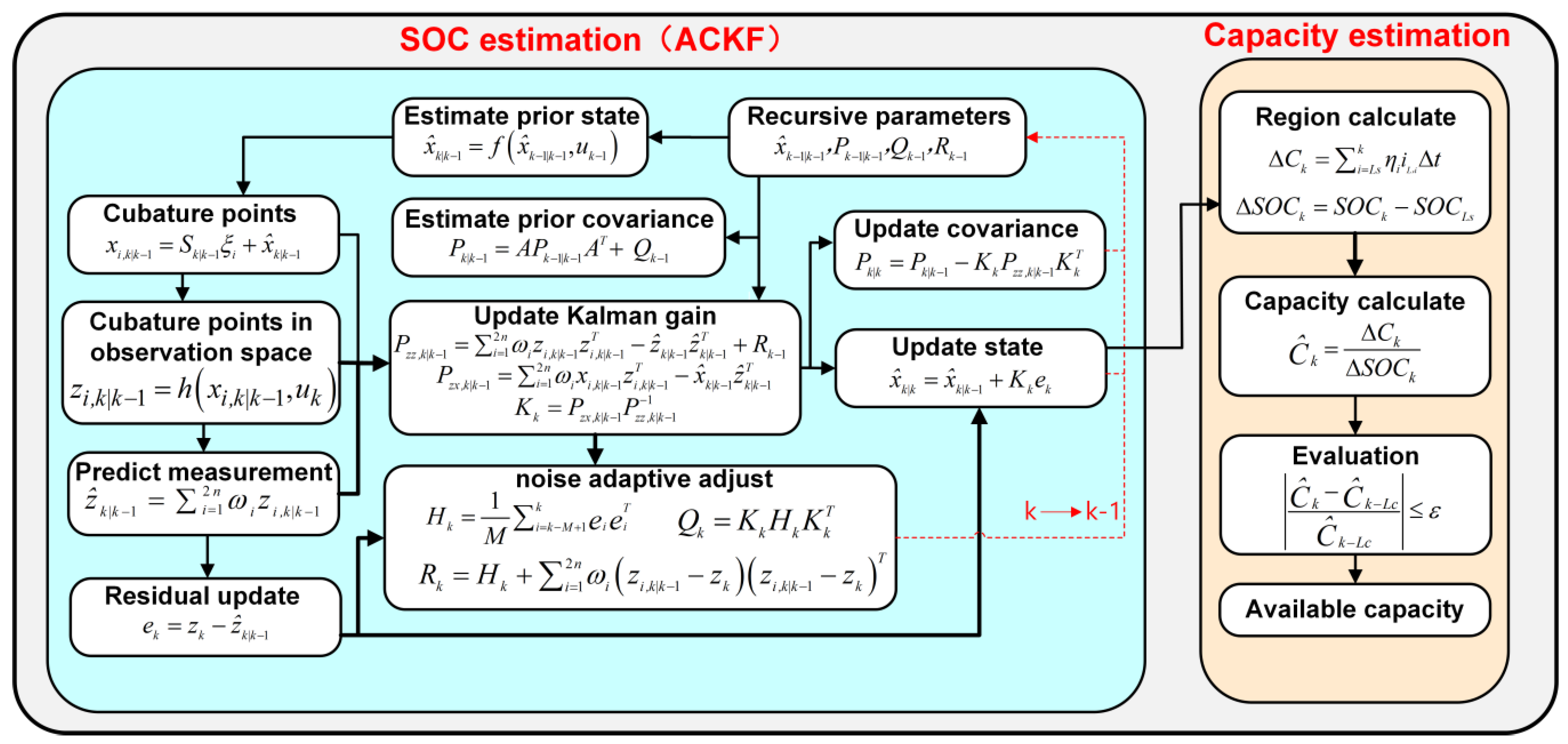
3.1. Adaptive Cubature Kalman Filter

The discrete state space equation of nonlinear system with additive noise is:
{ x k = f ( x k 1 , u k 1 ) + w k 1 z k = h ( x k , u k ) + v k
where xk denotes the state vector at step k; uk is the control input; f (·) and h (·) represent the process function and measurement function respectively; wk−1 and vk are independent Gaussian noise with zero mean, corresponding covariance are Qk−1 and Rk respectively. For the Thevenin model, the parameters and vectors in Equation (9) are defined as:
{ f ( x k , u k ) = A x k 1 + B u k 1 h ( x k , u k ) = O C V k U p , k R 0 i L , k 1 A = d i a g ( 1 , e x p ( Δ t R p   C p ) ) B = [ η Δ t C a R p ( 1 e x p ( Δ t R p   C p ) ) ] T x k = [ SOC k U p , k ] T z k = U t , k u k = i L , k
In order to cope with the nonlinearity, the distribution of random state vector is approximated by cubature points with uniform weight. Based on the spherical-radial cubature rule [33], the cubature points are generated through the following parameters:
{ ξ i = n [ 1 ] i ( i = 1 , 2 , , 2 n ) ω i = 1 / ( 2 n ) ( i = 1 , 2 , , 2 n )
where n denotes dimension of the state vector, ξi represents the ith cubature point, ωi denotes the weight of the ith points, [1] denotes the following set of points:
[ 1 ] = { [ 1 0 0 ] , , [ 0 0 1 ] , [ 1 0 0 ] , , [ 0 0 1 ] }

3.2. Process of SOC Estimation

As one component of xk, SOCk can be estimated online by the recurring following process:

3.2.1. Initialization

The mathematical expectation and covariance of state vector x0 need to be initialized as x ^ 0 | 0 and P0|0 respectively, and covariance Q0 and R0 are preset.

3.2.2. Time Update

The complete CKF generates the cubature points at step k − 1, and the cubature points are propagated to the state vector at step k by the process function. After averaging, the priori estimation at step k can be obtained. Due to the linearity of the Thevenin model process equation, the classic Kalman filter algorithm can be applied in the time update part, so that algorithm can be more concise and efficient. A hat over a letter denotes the estimation of corresponding parameter.
x ^ k | k 1 = f ( x ^ k 1 | k 1 , u k 1 ) = A x ^ k 1 | k 1 + B u k 1
P k | k 1 = A P k 1 | k 1 A T + Q k 1

3.2.3. Measurement Update

  • Generate cubature points:
    x i , k | k 1 = S k | k 1 ξ i + x ^ k | k 1 , ( i = 1 , 2 , , 2 n )
    P k | k 1 = S k | k 1 S k | k 1 T
    where Sk|k−1 is the Cholesky decomposition result of Pk|k−1.
  • Calculate propagated cubature points in observation space:
    z i , k | k 1 = h ( x i , k | k 1 , u k )
  • Calculate the predicted measurement:
    z ^ k | k 1 = i = 1 2 n ω i z i , k | k 1
  • Calculate the measurement innovation covariance:
    P z z , k | k 1 = i = 1 2 n ω i z i , k | k 1 z i , k | k 1 T z ^ k | k 1 z ^ k | k 1 T + R k 1
  • Calculate the cross-covariance:
    P z x , k | k 1 = i = 1 2 n ω i x i , k | k 1 z i , k | k 1 T x ^ k | k 1 z ^ k | k 1 T
  • Calculate the Kalman gain:
    K k = P z x , k | k 1 P z z , k | k 1 1
  • Calculate the updated state:
    x ^ k | k = x ^ k | k 1 + K k ( z k z ^ k | k 1 )
  • Calculate the updated covariance:
    P k | k = P k | k 1 K k P z z , k | k 1 K k T

3.2.4. Adaptive Update of Noise

According to the innovation sequence of terminal voltage, the process noise and measurement noise are adjusted adaptively.
  • The innovation covariance matrix:
    H k = 1 M i = k M + 1 k e i e i T
    where M denotes the window size which is defaulted as 60, ei denotes residual which is calculated by:
    e k = z k z ^ k | k 1
  • The process noise covariance Qk is updated as follows:
    Q k = K k H k K k T
  • The measurement noise covariance Rk is updated as follows:
    R k = H k + i = 1 2 n ω i ( z i , k | k 1 z k ) ( z i , k | k 1 z k ) T

3.3. Capacity Estimation Based on Estimated SOC

Based on the estimated SOC, the available capacity of battery can be estimated on-line. The capacity obtained through the capacity test is defaulted as the initial capacity value when SOC estimation starts to be performed. The change of capacity ΔCk and the change of SOC ΔSOCk are calculated as follows:
Δ C k = i = L s k η i i L , i Δ t
Δ S O C k = S O C k S O C L s
where Ls denotes the step at which the capacity estimation starts. That is, the capacity estimation starts only after the SOC estimation has passed Ls step so that fluctuation of capacity estimation is reduced during the initial period. The capacity is estimated by using following equation:
C ^ k = Δ C k Δ S O C k
In order to obtain a steady value of available capacity estimation, the change rate of capacity estimation is limited by using the following equation:
| C ^ k C ^ k L c C ^ k L c | ε
where ε denotes the acceptable change rate of capacity estimation, Lc denotes the step size of capacity estimation. That is, the capacity is estimated every Lc step. Once Equation (31) is not satisfied, the change between new estimated capacity and last estimated capacity will be compulsively set as ε.
Figure 7 illustrates the flowchart of SOC estimation and capacity estimation.

4. Experiment and Discussion
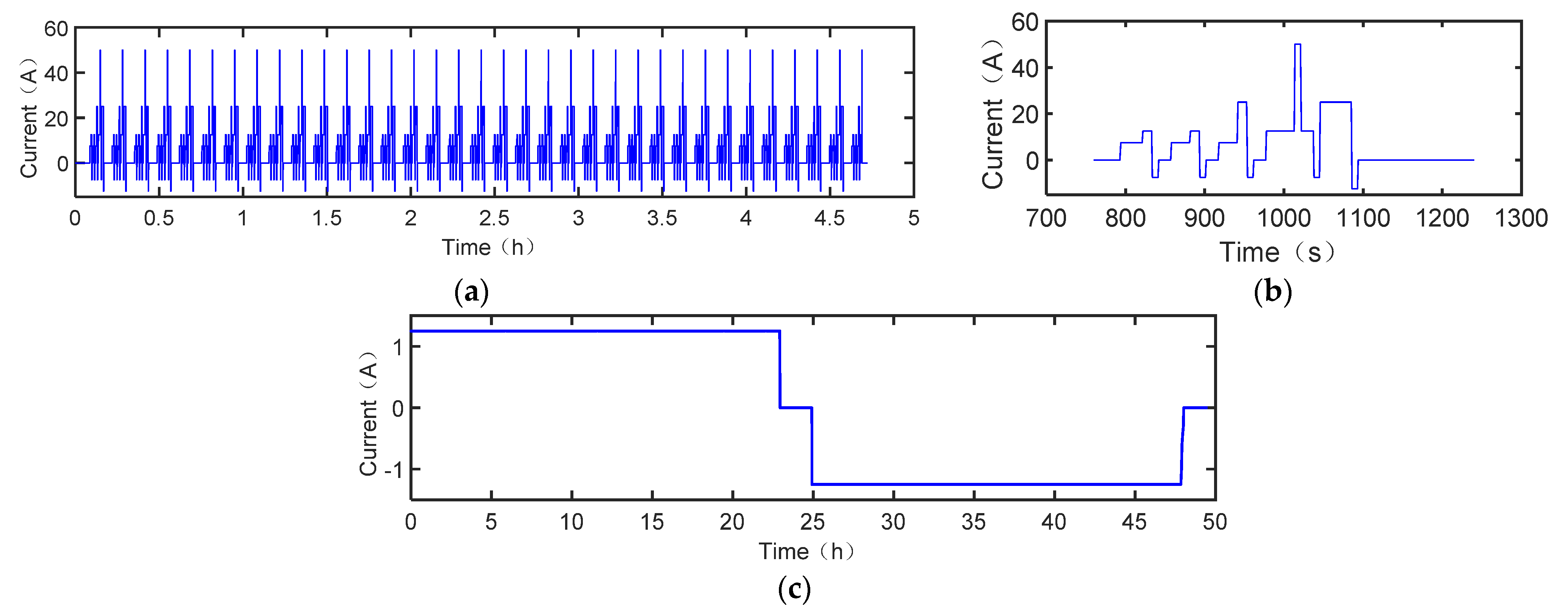
4.1. Experiment

The battery experimental system consisted of an Arbin BT2000 battery test machine, a thermal chamber and a computer with Arbin software. Tested NMC batteries and LFP batteries were manufactured by MGL. The capacity tests, OCV tests and dynamic stress tests (DST) were performed at the temperature of 10 °C, 25 °C, and 40 °C. Table 3 presents basic information of both batteries.
This study adopted a low-current OCV test, which stimulated the battery with 0.05 C, to obtain SOC–OCV data points with 1 Hz. SOC and capacity were estimated under DST which can emulate the actual driving cycles of EVs for batteries. The test profile of DST and low-current OCV test is illustrated in Figure 8.
Notably, OCV curves are regarded as OCV reference models whose OCV can be looked up in OCV curve table. In this way, the closeness between fusional OCV model and OCV curve model can be evaluated from the perspective of SOC estimation and capacity estimation.

4.2. The Fusional OCV Model

4.2.1. Fusional OCV Model of NMC Battery

The fitting results of fusional OCV models of the NMC battery at 10 °C, 25 °C and 40 °C are shown in Figure 9a,c,e. The fitting results of conventional OCV models in Table 4, which are same as the adopted sub-models, are shown in Figure 9b,d,e. All the OCV models fit the OCV curve based on 21 evenly distributed control points.
Table 5 shows the root mean squared error (RMSE) of all models. The fourth-degree polynomial OCV model performs worst, and what make it unbearable is that all the OCV fitting curves fourth-degree polynomial OCV model are non-monotonic. The OCV models 2, 3 can capture the changing trend of the OCV, but lost the precision in several local regions. Based on the local high-precision of sub-models, the fusional OCV model highly fits the experimental curve and corresponding RMSE is reduced dramatically. Compared with using OCV sub-models to fit the global OCV curve, the average accuracy of fusional OCV models increases about 2 times. In terms of temperature effect, the performance of fusional OCV model is not influenced by ambient temperature. Notably, in order to exclude the large error of OCV model when SOC drops to 0%, the SOC range of RMSE is between 5% and 100%.

4.2.2. Fusional OCV Model of LFP Battery

Similarly, the fusional OCV models of the LFP battery at 10 °C, 25 °C, and 40 °C are given in Figure 10a,c,e and the fitting results of OCV models in Table 4 are also given in Figure 10b,d,e. All the OCV models fit the OCV curve based on 21 evenly distributed control points. According to the RMSE of OCV models in Table 6, the fusional OCV models still perform with great precision, especially in the region of middle SOC. The fourth-degree polynomial OCV model is the most inaccurate and non-monotonic. Compared with using OCV sub-models to fit the global OCV curve, the average accuracy of fusional OCV model increases about 2 times. The OCV models 2, 3 can capture the changing trend of OCV. In terms of temperature effect, the performance of the fusional OCV model is not influenced by ambient temperature. Notably, in order to exclude the large error of the OCV model when SOC drops to 0% and rises to 100%, the SOC range of RMSE is between 5% and 99%.

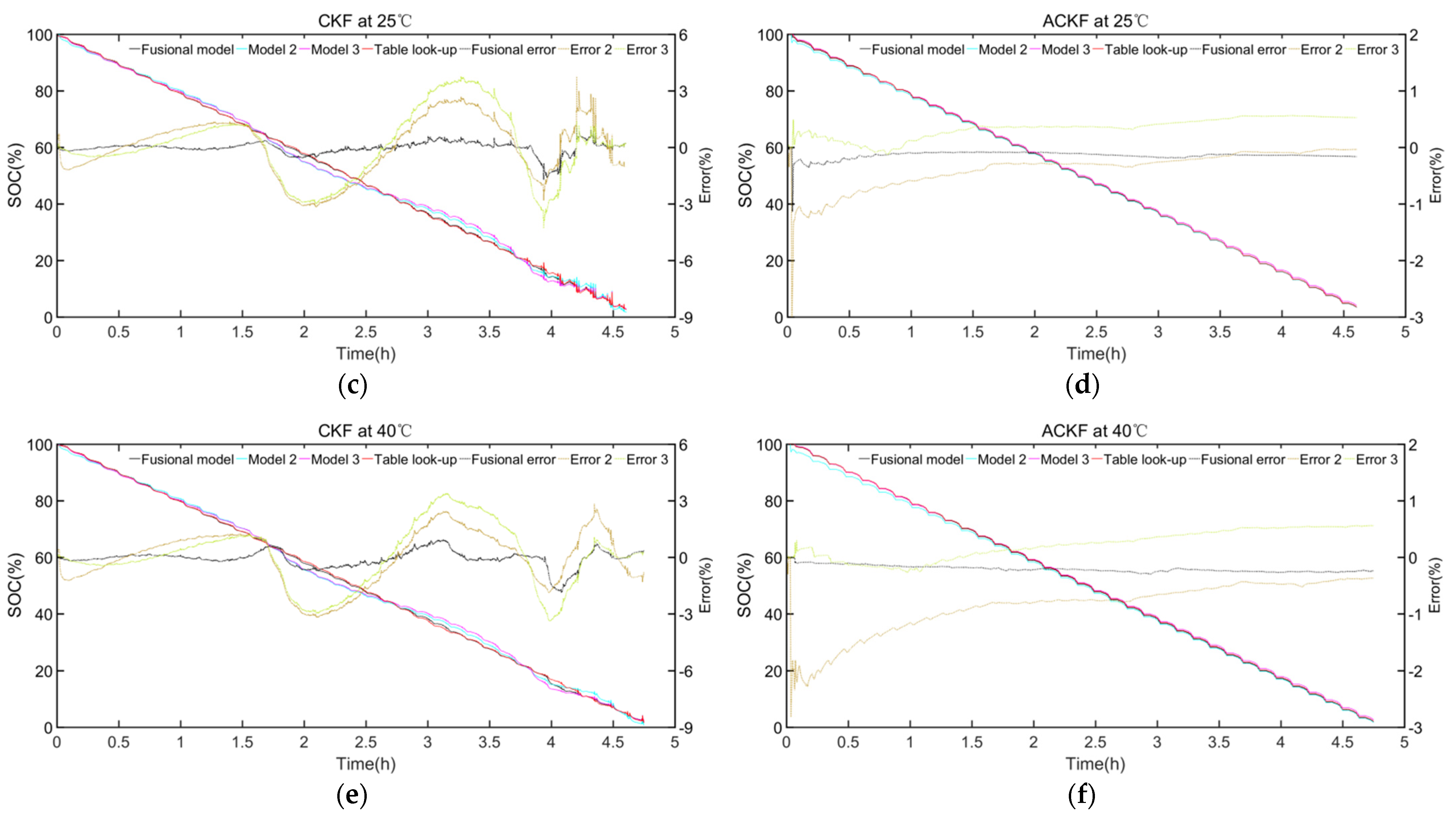
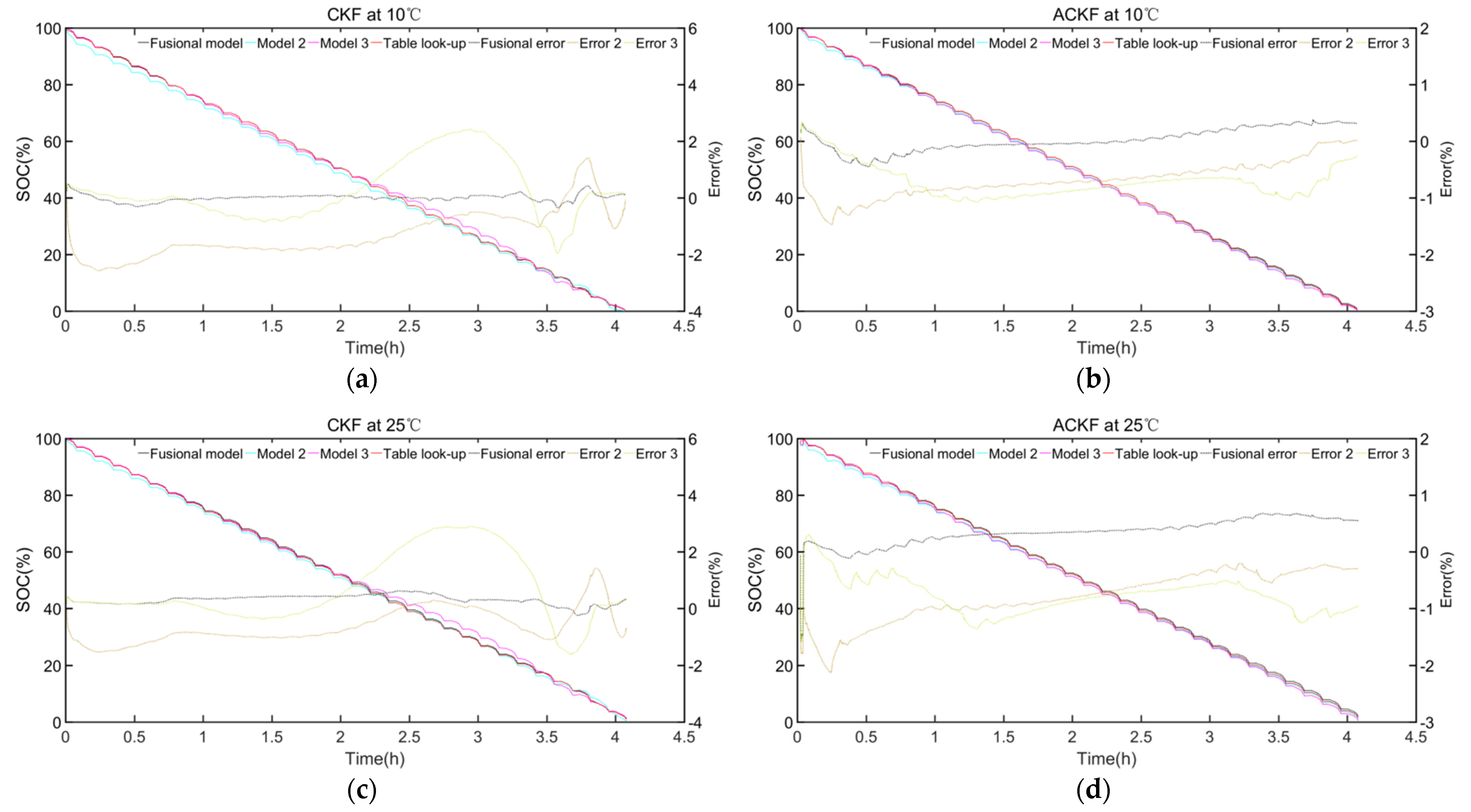
4.3. The Result of SOC Estimation with Different OCV Models

The proposed OCV model fusion method is further used to estimate SOC for verification of OCV model accuracy. By using CKF and ACKF to estimate SOC under DST at 10 °C, 25 °C and 40 °C, the estimation results of the NMC battery are shown in Figure 11 with corresponding RMSE in Table 7 and the estimation results of the LFP battery are given in Figure 12 with corresponding RMSE in Table 8. Due to the non-monotonicity and large error of fourth-degree polynomial OCV models, the corresponding SOC estimation results are invalid. The SOC estimation results of models 2 and 3 are considered.
When applying the CKF algorithm, the difference between the OCV models is obvious. Since the OCV curve of the NMC battery does not have the flat platform effect like LFP battery, the advantages of the fusion method are more beneficial for NMC battery. Compared with other models in the NMC battery, the SOC estimation error based on the fusional OCV model is dramatically reduced. For LFP battery, the SOC estimation error of fusional OCV models can still retain minimal, but error may fluctuate with temperature change. Overall, temperature has no significant effect on the fusion method. The addition of adaptive noise effectively weakens the influence of OCV model errors and stabilizes the estimation results. According to experimental result, the effect of the OCV model fusion method is verified.

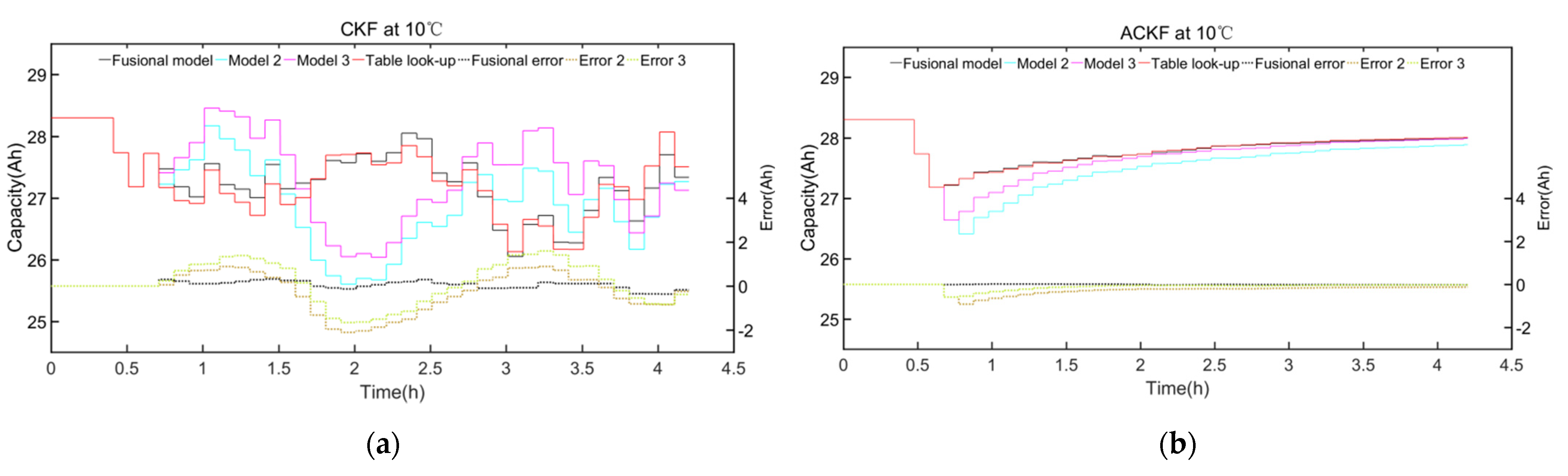
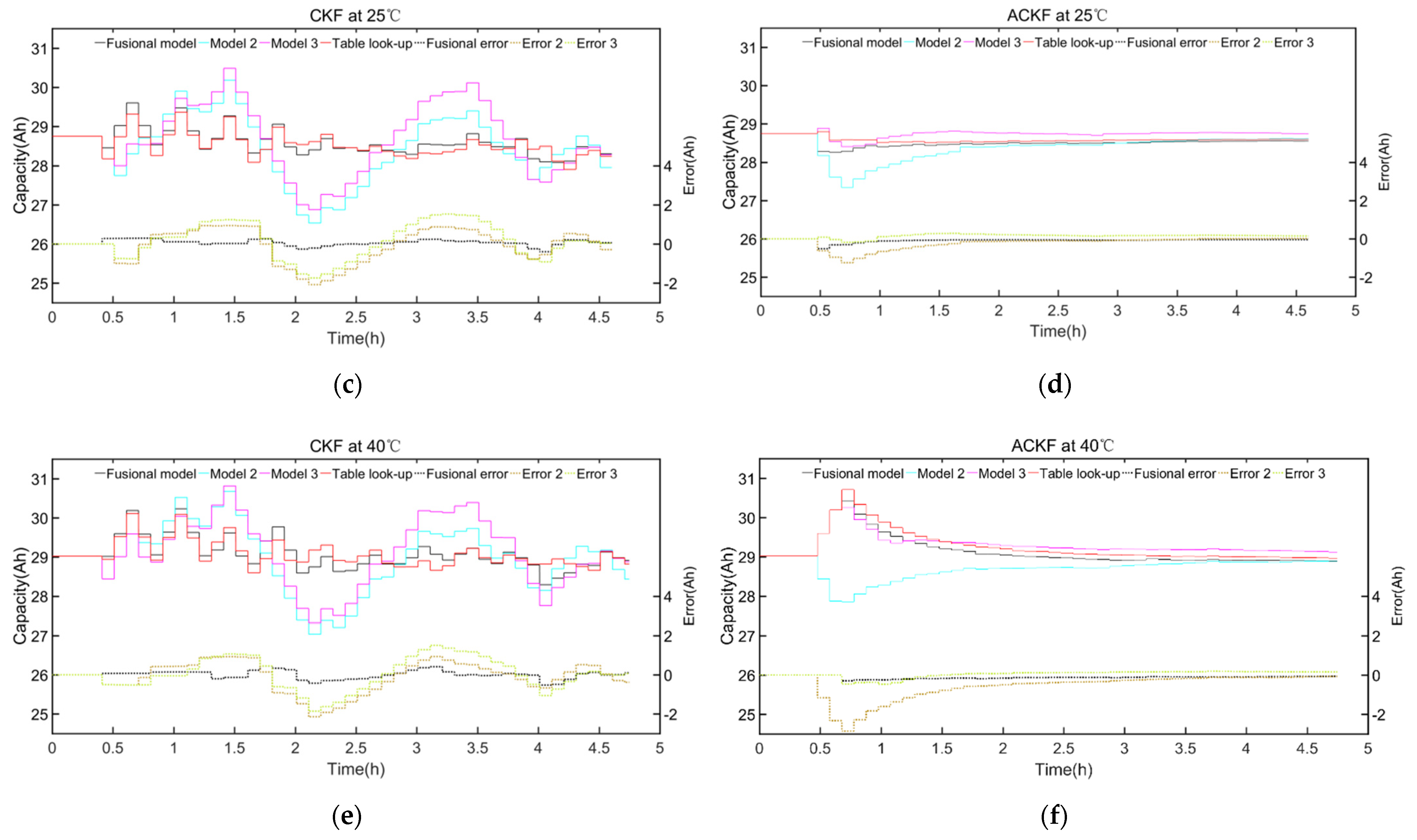
4.4. The Result of Capacity Estimation with Different OCV Models

In order to reduce the impact of the fluctuation during the initial period, capacity estimation starts to be performed after three DST cycles have finished. In consideration of the time cost of one DST cycle is 480 s in the experiment, start step LS is set as 1440 s. Cycle step Lc is set as 360 s and acceptable change rate ε is set as 2%. As shown in Figure 13 and Figure 14, it can be seen that fluctuation of capacity estimation by using the CKF algorithm is more obvious than capacity estimation by using the ACKF algorithm. What is more important, as shown in Table 9 and Table 10, is that fusional OCV models still perform best in tracking capacity estimation results of OCV curve models. In terms of temperature effect, ambient temperature has no significant effect on the OCV fusion method.

5. Conclusions

At present, the research on battery SOC and SOH estimation mainly focuses on improving the structure of an equivalent circuit model and proposing new estimation algorithms, ignoring the influence of the OCV model on the accuracy of state estimation. Using a single OCV model cannot have a good fitting effect in the entire battery discharge interval. For this reason, an OCV model fusion method is proposed that can effectively obtain a high-fidelity OCV model. The method makes it possible to focus on the fitting accuracy in a certain SOC interval, so as to capture the changing trend of the OCV in a specific SOC region as much as possible. Furthermore, it has good adaptability for fitting complex OCV curves, and provides a good solution for OCV curves that are difficult to fit globally. The generalization fitting performance of the method is verified by the application on NMC battery and LFP battery. Experimental results at three ambient temperatures showed that the performance of the fusional OCV model was not sensitive to temperature. Regarding the influence of the OCV fusion model on the accuracy of state estimation, this paper used CKF and ACKF to estimate the SOC and capacity under three ambient temperatures, the results indicating that the fusional OCV model can effectively track the performance of OCV curve model in terms of supporting algorithm.
The fusion method has an important implication for reconstructing a global OCV characteristic curve based on curve segments. It is not only suitable for offline low-current OCV experiments, and we will carry out research work on applying it to offline incremental OCV experiments and online OCV reconstruction processes.

Author Contributions

Conceptualization, C.W. and X.Z.; methodology, Q.Y.; software, L.E.; validation, T.L., and J.L.; writing—original draft preparation, Q.Y.; writing—review and editing, Y.H. and T.L.; All authors have read and agreed to the published version of the manuscript.

Funding

This work has been supported by the Shandong Provincial Natural Science Foundation Project (ZR2020ME209).

Institutional Review Board Statement

Not applicable.

Informed Consent Statement

Not applicable.

Data Availability Statement

Data sharing not applicable.

Acknowledgments

The systemic experiments of the lithium-ion batteries were performed at the Advanced Energy Storage and Application (AESA) Group, Beijing Institute of Technology.

Conflicts of Interest

The authors declare no conflict of interest.

References

  1. Abada, S.; Marlair, G.; Lecocq, A.; Petit, M.; Sauvant-Moynot, V.; Huet, F. Safety focused modeling of lithium-ion batteries: A review. J. Power Sources 2016, 306, 178–192. [Google Scholar] [CrossRef]
  2. Lai, X.; Zheng, Y.J.; Sun, T. A comparative study of different equivalent circuit models for estimating state-of-charge of lithium-ion batteries. Electrochim. Acta 2018, 259, 566–577. [Google Scholar] [CrossRef]
  3. Yang, R.; Xiong, R.; Shen, W.; Lin, X. Extreme Learning Machine Based Thermal Model for Lithium-ion Batteries of Electric Vehicles under External Short Circuit. Engineering 2020. [Google Scholar] [CrossRef]
  4. Yu, Q.; Xiong, R.; Yang, R.; Pecht, M. Online capacity estimation for lithium-ion batteries through joint estimation method. Appl. Energy 2019, 255, 113817. [Google Scholar] [CrossRef]
  5. Xing, Y.J.; He, W.; Pecht, M.; Tsui, K.L. State of charge estimation of lithium-ion batteries using the open-circuit voltage at various ambient temperatures. Appl. Energy 2014, 113, 106–115. [Google Scholar] [CrossRef]
  6. Hu, Y.; Yurkovich, S. Battery cell state-of-charge estimation using linear parameter varying system techniques. J Power Sources 2012, 198, 338–350. [Google Scholar] [CrossRef]
  7. Chemali, E.; Kollmeyer, P.J.; Preindl, M.; Emadi, A. State-of-charge estimation of Li-ion batteries using deep neural networks: A machine learning approach. J. Power Sources 2018, 400, 242–255. [Google Scholar] [CrossRef]
  8. Yu, Q.Q.; Xiong, R.; Wang, L.Y.; Lin, C. A Comparative Study on Open Circuit Voltage Models for Lithium-ion Batteries. Chin. J. Mech. Eng. 2018, 31, 64. [Google Scholar] [CrossRef] [Green Version]
  9. Fang, Y.; Xiong, R.; Wang, J. Estimation of Lithium-Ion Battery State of Charge for Electric Vehicles Based on Dual Extended Kalman Filter. Energy Procedia 2018, 152, 574–579. [Google Scholar] [CrossRef]
  10. Plett, G.L. Extended Kalman filtering for battery management systems of LiPB-based HEV battery packs: Part 3. State and parameter estimation. J. Power Source 2004, 134, 277–292. [Google Scholar] [CrossRef]
  11. Xiong, R.; Yu, Q.; Wang, L.Y. Open circuit voltage and state of charge online estimation for lithium ion batteries. Energy Procedia 2017, 142, 1902–1907. [Google Scholar] [CrossRef]
  12. Arasaratnam, I.; Haykin, S. Cubature Kalman filters. IEEE Trans. Autom. Control 2009, 54, 1254–1269. [Google Scholar] [CrossRef] [Green Version]
  13. Xiong, R.; Sun, F.C.; He, H.W. Data-driven state-of-charge estimator for electric vehicles battery using robust extended Kalman filter. Int. J. Automot. Technol. 2014, 15, 89–96. [Google Scholar] [CrossRef]
  14. Mohamed, A.H.; Schwarz, K.P. Adaptive Kalman filtering for INS/GPS. J. Geodesy 1999, 73, 193–203. [Google Scholar] [CrossRef]
  15. Han, J.; Kim, D.; Sunwoo, M. State-of-charge estimation of lead-acid batteries using an adaptive extended Kalman filter. J. Power Sources 2009, 188, 606–612. [Google Scholar] [CrossRef]
  16. Sun, F.C.; Hu, X.S.; Zou, Y.; Li, S.G. Adaptive unscented Kalman filtering for state of charge estimation of a lithium-ion battery for electric vehicles. J. Power Sources 2011, 36, 3531–3540. [Google Scholar] [CrossRef]
  17. Zheng, F.D.; Xing, Y.J.; Jiang, J.C.; Sun, B.X.; Kim, J.; Pecht, M. Influence of different open circuit voltage tests on state of charge online estimation for lithium-ion batteries. Appl. Energy 2016, 183, 513–525. [Google Scholar] [CrossRef]
  18. Petzl, M.; Danzer, M. Advancements in OCV Measurement and Analysis for Lithium-Ion Batteries. IEEE Trans. Energy Convers. 2013, 28, 675–681. [Google Scholar] [CrossRef]
  19. Zhu, J.G.; Knapp, M.; Darma, M.S.D.; Fang, Q.H.; Wang, X.Y.; Dai, H.F.; Wei, X.Z.; Ehrenberg, H. An improved electro-thermal battery model complemented by current dependent parameters for vehicular low temperature application. Appl. Energy 2019, 248, 149–161. [Google Scholar] [CrossRef]
  20. Lavigne, L.; Sabatier, J.; Francisco, M.; Guillemard, F.; Noury, A. Lithium-ion Open Circuit Voltage (OCV) curve modelling and its ageing adjustment. J. Power Sources 2016, 324, 694–703. [Google Scholar] [CrossRef]
  21. Plett, G.L. Extended Kalman filtering for battery management systems of LiPB-based HEV battery packs: Part 2. Modeling and identification. J. Power Sources 2004, 134, 262–276. [Google Scholar] [CrossRef]
  22. Xiong, R.; Li, L.; Yu, Q.; Jin, Q.; Yang, R. A set membership theory based parameter and state of charge co-estimation method for all-climate batteries. J. Clean. Prod. 2020, 249, 11389. [Google Scholar] [CrossRef]
  23. Xiong, R.; Sun, F.C.; Chen, C.; He, H.W. A data-driven multi-scale extended Kalman filtering based parameter and state estimation approach of lithium-ion polymer battery in electric vehicles. Appl. Energy 2014, 113, 463–476. [Google Scholar] [CrossRef]
  24. Dong, G.Z.; Wei, J.W.; Zhang, C.B.; Chen, Z.H. Online state of charge estimation and open circuit voltage hysteresis modeling of LiFePO4 battery using invariant imbedding method. Appl. Energy 2016, 162, 163–171. [Google Scholar] [CrossRef]
  25. Zhang, C.P.; Jiang, J.C.; Zhang, L.J.; Liu, S.J. A generalized SOC-OCV model for lithium-ion batteries and the SOC estimation for LNMCO battery. Energies 2016, 9, 900. [Google Scholar] [CrossRef] [Green Version]
  26. Hu, X.S.; Li, S.B.; Peng, H.; Sun, F.C. Robustness analysis of state-of-charge estimation methods for two types of Li-ion batteries. J. Power Sources 2012, 217, 209–219. [Google Scholar] [CrossRef]
  27. Ganesan, N.; Basu, S.; Hariharan, K.S.; Kolake, S.M.; Song, T.; Yeo, T.; Sohn, D.K.; Doo, S. Physics based modeling of a series parallel battery pack for asymmetry analysis, predictive control and life extension. J. Power Sources 2016, 322, 57–67. [Google Scholar] [CrossRef]
  28. Widanage, W.D.; Barai, A.; Chouchelamane, G.H.; Uddin, K.; McGordon, A.; Marco, J.; Jennings, P. Design and use of multisine signals for Li-ion battery equivalent circuit modelling. Part 2: Model estimation. J. Power Sources 2016, 324, 61–69. [Google Scholar] [CrossRef] [Green Version]
  29. Yu, Q.; Xiong, R.; Lin, C.; Shen, W.X.; Deng, J. Lithium-ion battery parameters and state-of-charge joint estimation based on H-infinity and unscented Kalman filters. IEEE Trans. Veh. Technol. 2017, 66, 8693–8701. [Google Scholar] [CrossRef]
  30. Hu, X.S.; Li, S.B.; Peng, H. A comparative study of equivalent circuit models for Li-ion batteries. J. Power Sources 2012, 198, 359–367. [Google Scholar] [CrossRef]
  31. Xiong, R.; Yu, Q.; Wang, L.; Lin, C. A novel method to obtain the open circuit voltage for the state of charge of lithium ion batteries in electric vehicles by using H infinity filter. Appl. Energy 2017, 207, 346–353. [Google Scholar] [CrossRef]
  32. Xiong, R. Estimation of Battery Pack State for Electric Vehicles Using Model-Data Fusion Approach. Ph.D. Thesis, Beijing Institute of Technology, Beijing, China, June 2014. [Google Scholar]
  33. Liu, M.; Lai, J.Z.; Li, Z.M.; Liu, J.Y. An adaptive cubature Kalman filter algorithm for inertial and land-based navigation system. Aerosp. Sci. Technol. 2016, 51, 52–60. [Google Scholar] [CrossRef]
Figure 1. Thevenin model.
Energies 14 01797 g001
Figure 2. Conventional open circuit voltage (OCV) models for LiNiMnCoO2 (NMC) battery (21 control points, s denotes state of charge (SOC), k0, 1, 2, 3, 4, α, β denote fitting coefficients). (a) Fourth-degree polynomial. (b) Polynomial and logarithm. (c) Exponent and linear function.
Energies 14 01797 g002
Figure 3. Flowchart of OCV model fusion method.
Energies 14 01797 g003
Figure 4. An OCV curve of a NMC battery with changing rate of OCV over SOC.
Energies 14 01797 g004
Figure 5. An OCV curve of LiFePO4 (LFP) battery with changing rate of OCV over SOC.
Energies 14 01797 g005
Figure 6. Conventional OCV models for LFP battery (21 control points, s denotes SOC, k0, 1, 2, 3, 4, α, β denote fit coefficients). (a) Fourth-degree polynomial. (b) Polynomial and logarithm. (c) Exponent and linear function.
Energies 14 01797 g006
Figure 7. Flowchart of state of charge (SOC) and capacity estimation.
Energies 14 01797 g007
Figure 8. Current profiles of: (a) DST. (b) Cycle window of DST. (c) low-current OCV test.
Energies 14 01797 g008
Figure 9. OCV models of NMC battery at 10 °C, 25 °C, and 40 °C. (a) Fusional OCV model at 10 °C. (b) Conventional OCV models at 10 °C. (c) Fusional OCV model at 25 °C. (d) Conventional OCV models at 25 °C. (e) Fusional OCV model at 40 °C. (f) Conventional OCV models at 40 °C.
Energies 14 01797 g009aEnergies 14 01797 g009b
Figure 10. OCV models of LFP battery at 10 °C, 25 °C, and 40 °C. (a) Fusional OCV model at 10 °C. (b) Conventional OCV models at 10 °C. (c) Fusional OCV model at 25 °C. (d) Conventional OCV models at 25 °C. € Fusional OCV model at 40 °C. (f) Conventional OCV models at 40 °C.
Energies 14 01797 g010aEnergies 14 01797 g010b
Figure 11. SOC estimation results for NMC battery by using: (a) CKF at 10 °C. (b) ACKF at 10 °C. (c) CKF at 25 °C. (d) ACKF at 25 °C. (e) CKF at 40 °C. (f) ACKF at 40 °C.
Energies 14 01797 g011aEnergies 14 01797 g011b
Figure 12. SOC estimation results for LFP battery by using: (a) CKF at 10 °C. (b) ACKF at 10 °C. (c) CKF at 25 °C. (d) ACKF at 25 °C. (e) CKF at 40 °C. (f) ACKF at 40 °C.
Energies 14 01797 g012aEnergies 14 01797 g012b
Figure 13. Capacity estimation results for NMC battery by using: (a) CKF at 10 °C. (b) ACKF at 10 °C. (c) CKF at 25 °C. (d) ACKF at 25 °C. (e) CKF at 40 °C. (f) ACKF at 40 °C.
Energies 14 01797 g013aEnergies 14 01797 g013b
Figure 14. Capacity estimation results for LFP battery by using: (a) CKF at 10 °C. (b) ACKF at 10 °C. (c) CKF at 25 °C. (d) ACKF at 25 °C. (e) CKF at 40 °C. (f) ACKF at 40 °C.
Energies 14 01797 g014aEnergies 14 01797 g014b
Table 1. Sub-models of NMC battery.
Sub-IntervalSub-Model
(0, 25%) O C V N M C , 1 ( s ) = k 0 + k 1 s + k 2 ( 1 e x p ( α s ) ) + k 3 ( 1 e x p ( β / ( 1 s ) ) )
(15, 70%) O C V N M C , 2 ( s ) = k 0 + k 1 s + k 2 s 2 + k 3 s 3 + k 4 s 4
(60, 100%) O C V N M C , 3 ( s ) = k 0 + k 1 s + k 2 s 2 + k 3 s 3 + k 4 s 4
Table 2. Sub-models of LFP battery.
Sub-IntervalSub-Model
(0, 25%) O C V L F P , 1 ( s ) = k 0 + k 1 s + k 2 ( 1 e x p ( α s ) ) + k 3 ( 1 e x p ( β / ( 1 s ) ) )
(15, 85%) O C V L F P , 2 ( s ) = k 0 + k 1 s + k 2 s 2 + k 3 s 3 + k 4 log ( s ) + k 5 ( 1 s )
(75, 100%) O C V L F P , 1 ( s ) = k 0 + k 1 s + k 2 ( 1 e x p ( α s ) ) + k 3 ( 1 e x p ( β / ( 1 s ) ) )
Table 3. Basis information of tested batteries.
MaterialTypeNominal Capacity (Ah)Available Capacity (Ah)
10 °C25 °C40 °C
NMCcylinder25.0028.3028.7529.02
LFPpouch20.0019.7219.8519.94
Table 4. Conventional OCV models.
LabelModel
1 O C V 1 ( s ) = k 0 + k 1 s + k 2 s 2 + k 3 s 3 + k 4 s 4
2 O C V 2 ( s ) = k 0 + k 1 s + k 2 s 2 + k 3 s 3 + k 4 log ( s ) + k 5 ( 1 s )
3 O C V 3 ( s ) = k 0 + k 1 s + k 2 ( 1 e x p ( α s ) ) + k 3 ( 1 e x p ( β / ( 1 s ) ) )
Table 5. RMSE of fusional OCV models and other models for NMC battery (V).
10 °C25 °C40 °C
Fusional model0.00220.00270.0031
Model 10.04730.05750.0596
Model 20.01060.01150.0117
Model 30.01090.01050.0101
Table 6. RMSE of fusional OCV models and other models for LFP battery (V).
10 °C25 °C40 °C
Fusional model0.00320.00330.0033
Model 10.03860.04820.0782
Model 20.00880.01010.0100
Model 30.00900.00960.0106
Table 7. RMSE of SOC estimation for NMC battery (%).
10 °C25 °C40 °C
CKFACKFCKFACKFCKFACKF
Fusional model0.32770.07250.33850.15550.44650.2125
Model 21.63780.60271.54540.50561.45080.9889
Model 31.94070.18431.77820.38281.62610.3358
Table 8. RMSE of SOC estimation for LFP battery (%).
10 °C25 °C40 °C
CKFACKFCKFACKFCKFACKF
Fusional model0.64620.20490.35300.41790.65060.2905
Model 21.62220.75260.87400.91571.47140.7377
Model 31.20800.76561.37790.83552.41030.3655
Table 9. RMSE of capacity estimation for NMC battery (Ah).
10 °C25 °C40 °C
CKFACKFCKFACKFCKFACKF
Fusional model0.18330.01380.17180.15560.22260.1427
Model 20.93950.35580.88010.43170.81610.9693
Model 30.98770.19730.94140.19400.84990.1866
Table 10. RMSE of capacity estimation for LFP battery (Ah).
10 °C25 °C40 °C
CKFACKFCKFACKFCKFACKF
Fusional model0.15230.18660.10730.17910.28080.1240
Model 20.62950.40620.47530.24610.54420.3240
Model 30.37750.48500.43070.41020.84650.1283
Publisher’s Note: MDPI stays neutral with regard to jurisdictional claims in published maps and institutional affiliations.

