Comparison of Two Solar Probabilistic Forecasting Methodologies for Microgrids Energy Efficiency

Abstract

In this paper, the performances of two approaches for solar probabilistic are evaluated using a set of metrics previously tested by the meteorology verification community. A particular focus is put on several scores and the decomposition of a specific probabilistic metric: the continuous rank probability score (CRPS) as they give extensive information to compare the forecasting performance of both methodologies. The two solar probabilistic forecasting methodologies are used to produce intra-day solar forecasts with time horizons ranging from 1 h to 6 h. The first methodology is based on two steps. In the first step, we generated a point forecast for each horizon and in a second step, we use quantile regression methods to estimate the prediction intervals. The second methodology directly estimates the prediction intervals of the forecasted clear sky index distribution using past data as inputs. With this second methodology we also propose to add solar geometric angles as inputs. Overall, nine probabilistic forecasting performances are compared at six measurements stations with different climatic conditions. This paper shows a detailed picture of the overall performance of the models and consequently may help in selecting the best methodology.

1. Introduction

The increasing of electric energy coming from solar systems into electricity grids may affect the balance between demand and supply in the grid. In this case, grid operators could require additional energy reserves or conventional thermal electric plants to ensure the stability of the grid. In this context, forecasts of the solar irradiance and consequently of the solar power output at several time horizons are important to manage the balance of the grid [1,2,3].

Numerous studies have been developed using point forecast (deterministic forecast) models [4,5,6,7]. By definition, a forecast presents an uncertainty associated to the error compared with the real data. The knowledge of the point forecast prediction intervals could lead to a better decision-making process for a grid operator. We can find a wide literature about probabilistic forecasting for wind power [8,9,10] or solar energy prediction [11,12,13]. It is possible to reference these models according to their forecasting time horizons.

Models based on numerical weather predictions (NWP) mostly offer the best results for time horizons from 6 h to several days ahead. Some models assess the prediction intervals using a post-processing of the deterministic forecasts generated by the NWP model, by using a linear fitting model to obtain standard deviation of solar forecasting provided by European Centre for Medium-Range Weather Forecasts (ECMWF) [4] or by developing an ensemble approach using Regional Atmospheric Modeling System (RAMS) data [14]. GEFCom 2014 [15] proposed to generate PV power output probabilistic forecasts for 24 h ahead at three locations in Australia. The most interesting models to develop 99 quantiles were the multiple quantile regression [16], the gradient boosting technique, the K-nearest neighbors [17], and the quantile regression forest combined with gradient boosting decision trees [18].

Another group of models also provides ensemble forecasts using a set of perturbed NWP forecasts, ensemble prediction system (EPS). Sperati et al. (2016) [19] proposed a variance deficit (VD), using a logit transform and the ensemble model output statistics (EMOS) [20]. In the same way, Zamo et al. (2014) [21] compared two different quantile regression models using the Météo France’s ensemble NWP system (PEARP).

For time horizons ranging from 2 h to 6 h, forecasting models based on satellites images as inputs obtained better results. However, in the field of solar radiation probabilistic forecasting, only few studies have been published using models derived from satellite images combined with ground data, Alonso-Suarez et al. (2020) [22].

Finally, grid operators need time horizons from several seconds to several hours forecasting for decision-making in real time. In this range of horizons, most common models are based on two methodologies: models based on sky images from ground-based cameras or statistical models based on time series. Using sky images and past ground data, Pedro and Coimbra (2015) [23] proposed a k-nearest-neighbors (kNN) algorithm for global horizontal irradiance (GHI) intra-hour forecasting. Chu and Coimbra (2016) [24] generated very short-term Direct Normal Irradiance (DNI) probabilistic forecasting also based on the kNN and sky images.

In the group of statistical models, some papers dealt only based on past ground data to produce probabilistic forecasts. Bacher et al. (2009) [25] post-processed a deterministic forecast obtained from an autoregressive model using a weighted quantile regression based on a Gaussian kernel. Iversen et al. (2014) [26] proposed a stochastic differential equation (SDE) both for wind power and GHI forecasting. Similarly, David et al. (2016) [27] used an ARMA model for the point forecasts and a GARCH model for the probabilistic forecasts. Finally, Grantham et al. [28] proposed a Sieve Bootstrap method to post-treat the point forecasts obtained with an autoregressive model. As in the previous models, David et al. (2018) [29] did a comparison of 20 intraday solar probabilistic models using only past GHI data to generate the point forecasts. In a second step, a probabilistic approach was used to estimate the solar irradiance probabilistic forecasting. In their conclusion, the authors stated that none of the combination of the models clearly outperformed the other ones.

Furthermore, in the solar community it is possible to find several studies discussing verification tools to compare the results using different techniques. Lauret et al. (2019) [30] established a useful and wide comparison of different metrics and graphical tools for quantile forecasts and EPS probabilistic forecasting and Yang et al. (2020) [31] presented different verification metrics for deterministic forecasting.

In the literature, we can find two main methodologies to obtain solar probabilistic forecasting widely tested whatever the time horizon: post-processing of a previous deterministic forecasting or a direct generation of quantile intervals. In this paper, we will compare these two different methodologies for the first time. The first one only uses six past events from measured data to obtain the point forecast in a first step and, in a second step, a forecasted quantile regression distribution using the point forecast. On the contrary, methodology 2 obtains a set of forecasted quantiles directly with a quantile regression model. Regarding methodology 2, this paper proposes two variants. A first variant uses only past measured data as inputs, while the second variant includes zenith and hour angle as inputs for each model.

The methodology 1, based on the post-processing of a point forecast with a quantile regression model, will use the best models pointed by David et al. (2018) [29]. The second methodology intends to directly generate the quantiles of the forecasted clear sky index using different quantile regression methods. Furthermore, we will also test the improvement brought by the addition of the solar path (i.e., zenith and hour angles) as inputs to the probabilistic models. But the use of these exogenous inputs will be done only for the second approach which generates the quantiles in one step. The assessment of the probabilistic forecasts is obtained using a wide range of verification metrics recommended by the community. In this case, we used six different locations that represent a large variety of climates around the world.

In this work, we recall that our goal is to compare methodology 1 against methodology 2 to provide detailed information about different forecasting distribution at a certain location. This paper is summarized in the following sections. Section 2 describes the data used to build and test the different models. Section 3 presents the methodologies used to generate the probabilistic forecasts and both point and probabilistic models. Section 4 proposes a description of the probabilistic error metrics. Finally, Section 5 presents and discusses the results of both probabilistic forecasting methodologies and Section 6 offers some conclusions and future remarks.

2. Data

In this work, we used ground measurement data obtained from six different stations around the world. This set of measured data has been prepared for previous works aiming to develop and to compare solar probabilistic forecasting models [29,30]. These six locations present very different climate conditions, see

Table 1. Main characteristics of the six measurement stations.

	Desert Rock (USA)	Fort Peck (USA)	Fouillole (Guadeloupe)	Oahu (Hawaii)	Saint-Pierre (Reunion)	Tampon (Reunion)
Provider	SURFRAD		NREL	LARGE	PIMENT
Position	36.6 N 119.0 W	48.3 N 105.1 W	16.6 N 61.5 W	21.3 N 158.1 W	21.3 S 55.5 E	21.3 S 55.5 E
Elevation	1007 m	634 m	6 m	11 m	75 m	550 m
Climate type	Desert	Continental	Insular tropic	Insular tropic	Insular tropic	Insular heights
Training year	2012 2013	2012 2013	2010 2011	2010 2011	2012 2013	2012 2013
Testing year
Annual solar irradiance (MWh/m2)	2.105	1.447	1.893	1.969	2.053	1.712
Solar variability 1-h $(\mathsf{\sigma }\Delta {\mathrm{kt}}_{1\mathrm{h}}^{*}$)	0.146	0.181	0.213	0.209	0.191	0.241

. For this study, we computed 1-h averages of GHI using two consecutive years of 1-min measurements at each location. The first year for each location represents the training dataset, while the second year is the testing dataset. Measured data obtained with solar zenith angle (SZA) over 80º present large uncertainties associated to irradiance devices. Indeed, we filtered out nighttime data over 80° SZA from the datasets. Moreover, GHI measured were preprocessed to avoid gaps and measurement errors [27].

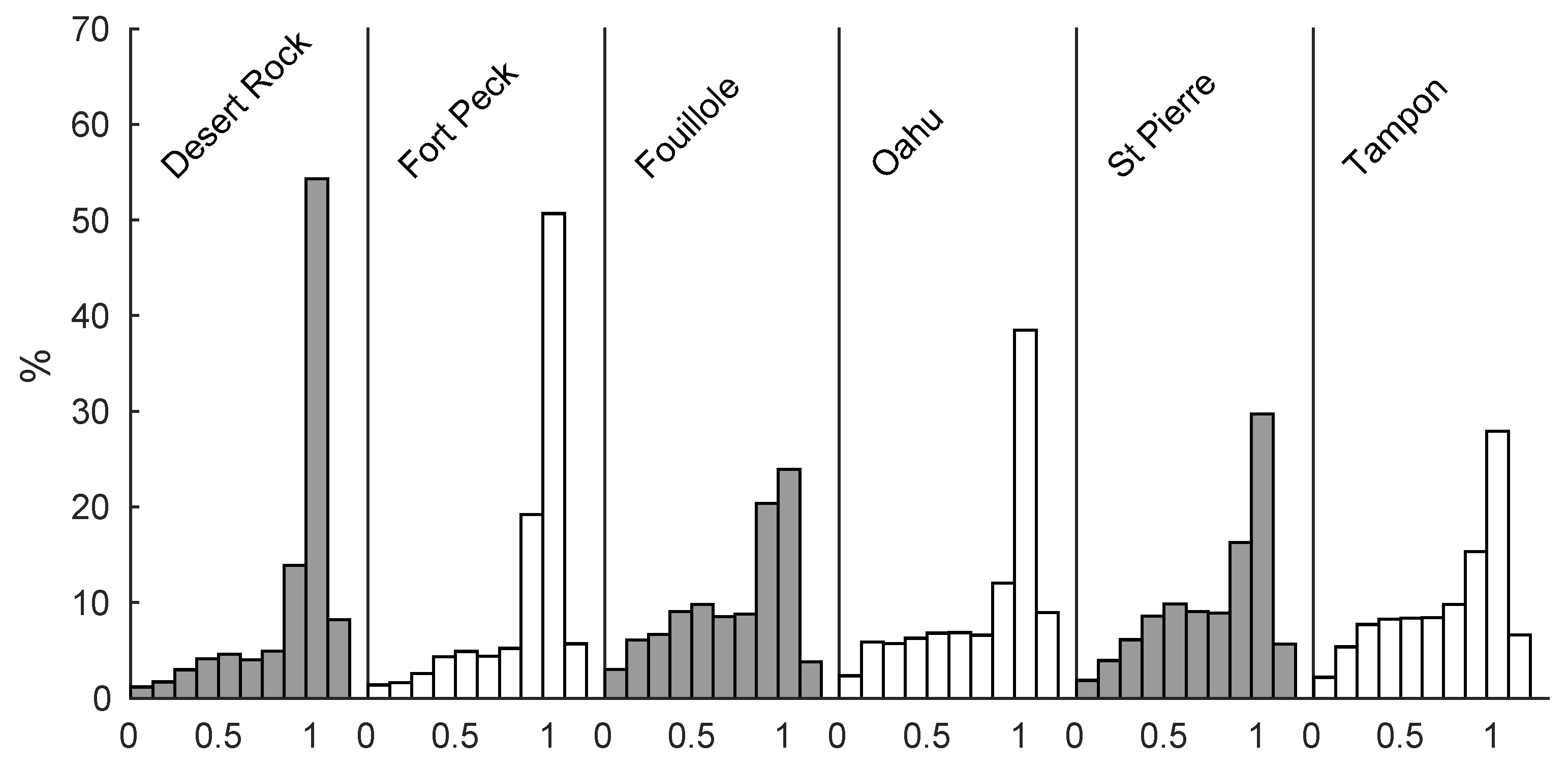
To obtain a better knowledge of GHI characteristics in these different stations, Figure 1 plots the clear sky index distribution. It is possible to notice in Figure 1 a significant number of over irradiance data, a clear sky index above 1. This fact can be observed in many measurement stations around the world [32]. Table 1 gives the solar variability as the standard deviation of the changes in the clear sky index ($\sigma \Delta k{t}_{\Delta t}^{*}$) with 1-h step [33]. Desert Rock and Fort Peck, continental locations, show a high frequency of clear skies moments and low solar variability. By contrast, the four insular stations, with tropical climates, present a higher variability and low occurrence of clear skies. Lauret, Voyant et al. (2015) [7] showed that variability affects the accuracy of solar radiation point forecasting.

GHI time series can be characterized by a deterministic part, diurnal and annual cycles, and a stochastic part [34]. Forecasting models pretend to obtain accurate results to predict the stochastic part of GHI, as the one caused by clouds. Indeed, all models used in this paper do not work with GHI directly. We computed clear sky index ($k{t}^{*}$) to eliminate the deterministic part (Equation (1)). The resulting time series is almost stationary.

$$k{t}^{*}=\frac{GHI}{GH{I}_{Clear}}$$

(1)

where $k{t}^{*}$ is the measured GHI divided by estimated GHI in clear sky day. This variable represents the deterministic part of the GHI. In this work, we use the clear sky data provided by the McClear model [35] available for free on the SoDa website [36]. This model uses the AODs, water vapor, and ozone date from the MACC project.

3. Methodologies and Forecasting Models Description

In this work, a set of quantile forecasts describes the uncertainty related to GHI forecast [37,38]. All methods described below produce this set of quantiles using regression models. In this section, forecasting models used in this paper are presented. In general, the equations use the following notation: (^) is a forecast variable, h is the desired time horizon, and t establishes the time when the forecasts are generated.

First, we define the probability meaning of a quantile level τ (0 ≤ τ ≤ 1):

$$q_{\tau }=F^{-1}\left(\tau \right)=\inf \left\{y:F\left(y\right)\ge \tau \right\}$$

(2)

For a random variable Y, F is the cumulative probability distribution (CDF):

$$F\left(y\right)=\mathrm{Pr}\left(\mathrm{Y}\le \mathrm{y}\right)$$

(3)

Indeed, a τ-quantile $q_{\tau }$ shows a τ probability of finding a measurement below the quantile $q_{\tau }$. Using a quantile set, we can define the prediction intervals. In this study we estimate the central prediction intervals [37]. For instance, a prediction interval of 90% is defined by the following equation:

$$I_{95\%}=\left[q_{\tau =0.05},q_{\tau =0.95}\right]$$

(4)

For GHI probabilistic forecasting, we will generate a different set of quantiles for each time horizons h. Therefore, regression methods used in this paper estimate a set of quantiles ${\left\{\widehat{q_{\tau }}\left(t+h\right)\right\}}_{\tau =0.1,0,2,\cdots ,0.9}$ for each forecasting time horizon $h=1,2,\cdots 6.$ In the following, this set of quantiles is composed of clear sky indices that are further transformed into a set of GHI quantiles using Equation (1). This set of quantiles may form an evenly spaced ensemble prediction system (EPS), as defined by the verification weather community [39].

3.1. Description of Two Methodologies to Generate Quantile Forecasts

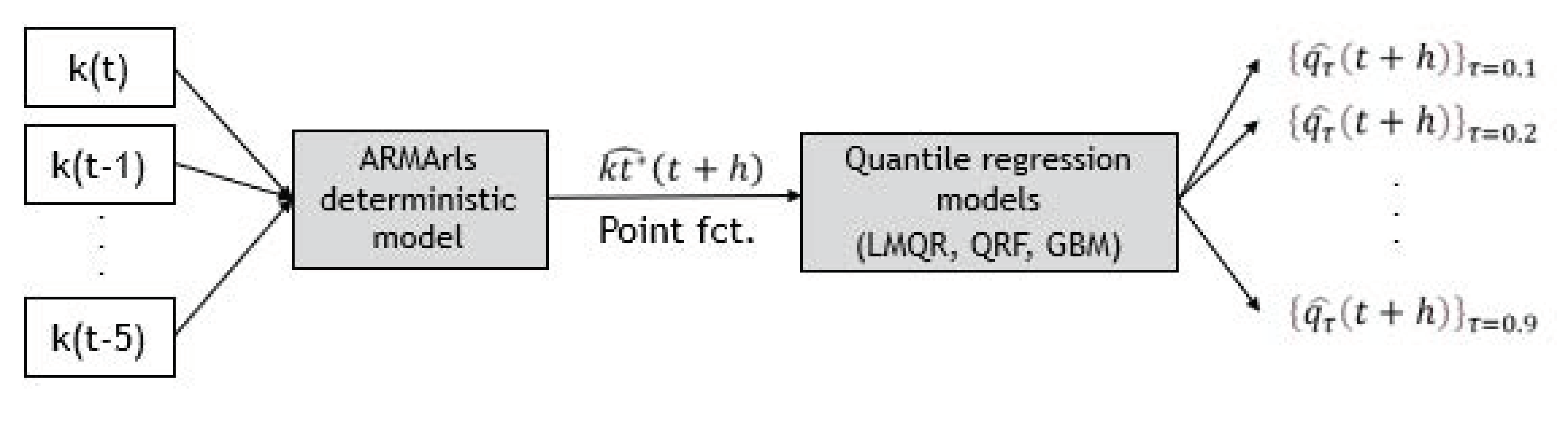
3.1.1. Methodology 1: Determinist + Post-Treatment

This first methodology has been proposed by Bacher 2009 [25] and has been tested on several sites [29]. In a first step, a point forecast at time horizon h, $\widehat{k{t}^{*}}\left(t+h\right)$ is produced and in a second step, a quantile regression method is used to estimate the set of quantiles. The point forecast is provided by the ARMArls method described in Section 4.1. This ARMArls uses six past measured radiation data as inputs, $k^{*}{\left(t-j\right)}_{j=0,1,\dots 5}$.

In this experimental set-up, the quantile regression models, depicted in Section 4.2, use only one predictor variable, the point forecasts of time horizon h, $\widehat{k{t}^{*}}\left(t+h\right)$ generated by ARMArls model, for generating the set of estimated quantiles ${\left\{\widehat{q_{\mathsf{\tau }}}\left(t+h\right)\right\}}_{\tau =0.1,0,2,\cdots ,0.9}$ for each forecasting time horizon h (see Figure 2).

$${\left\{\widehat{q_{\tau }}\left(t+h\right)\right\}}_{\tau =0.1,0,2,\cdots ,0.9}=f_q\left(\widehat{k{t}^{*}}\left(t+h\right)\right)\mathrm{for}h=1,2,\cdots ,6$$

(5)

In the preceding equation, the functional form $f_q$ stands for the quantile regression methods used to estimate the set of quantiles. This methodology in described and tested in [27,29].

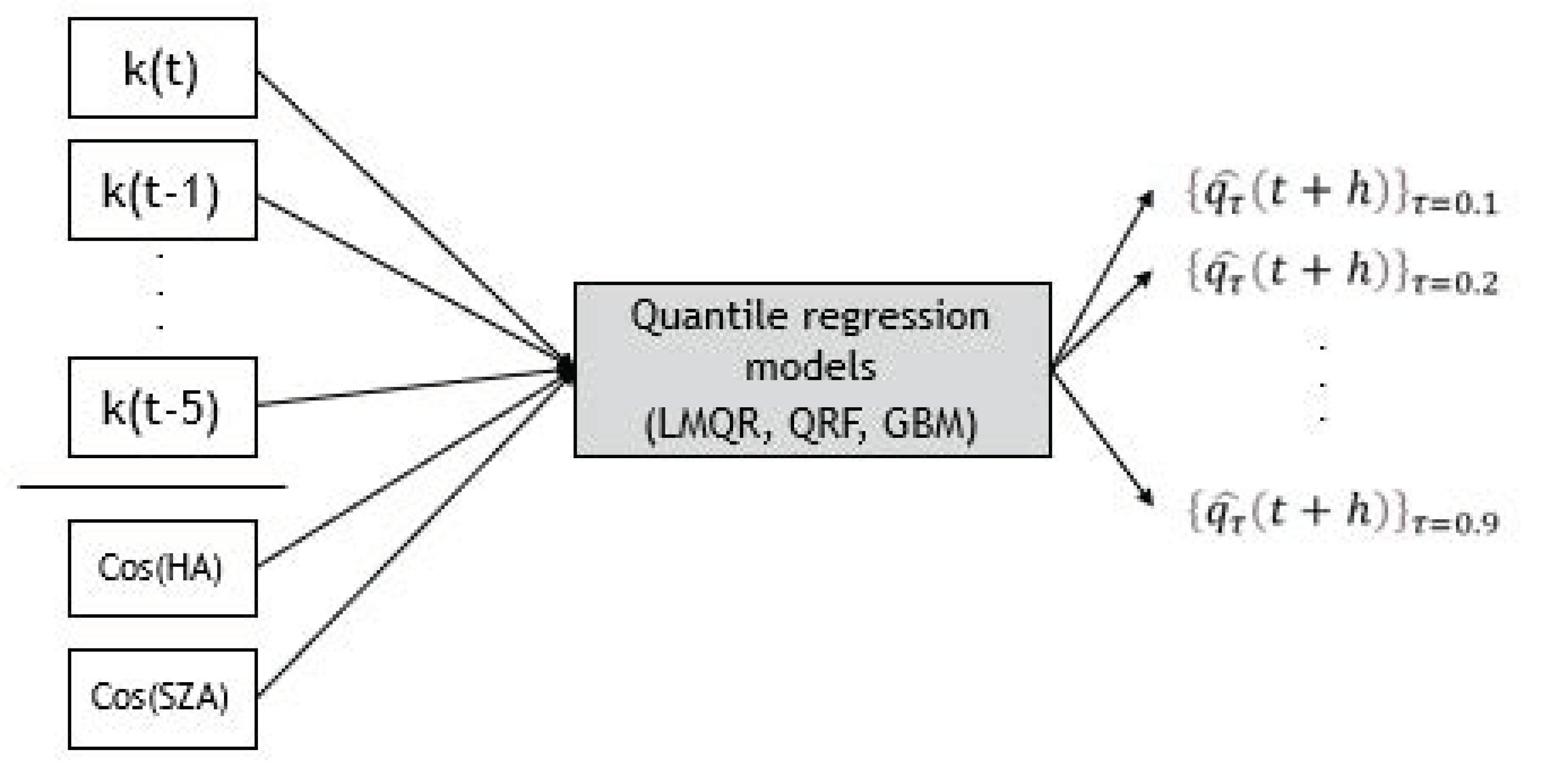
3.1.2. Methodology 2: Direct Generation of Quantiles

For the second methodology, we directly estimate the set of forecasted quantiles, ${\left\{\widehat{q_{\tau }}\left(t+h\right)\right\}}_{\tau =0.1,0,2,\cdots ,0.9}$, using a quantile regression model to relate input variables with the clear sky at forecasting time horizon h. Two experimental set-ups related to different types of regression models will be assessed. The first quantile regression model, variant 1, is based on Equation (6) and generates the set of quantiles directly from the six past ground measurements, $k^{*}{\left(t-j\right)}_{j=0,1,\dots 5}$.

$${\left\{\widehat{q_{\tau }}\left(t+h\right)\right\}}_{\tau =0.1,0,2,\cdots ,0.9}=f_q\left(k^{*}\left(t\right),k^{*}\left(t-1\right),\cdots ,k^{*}\left(t-p\right)\right)\mathrm{for}h=1,2,\cdots ,6$$

(6)

While the second variant of methodology 2 adds two geometrical solar angles as inputs. In this case, we used the cosine of the zenith angle $\cos \left(SZA\right)$ and the cosine of the hour angle $\cos \left(HA\right)$ because they describe the sun position in the sky:

$${\left\{\widehat{q_{\tau }}\left(t+h\right)\right\}}_{\tau =0.1,0,2,\cdots ,0.9}=f_q\left(k^{*}\left(t\right),k^{*}\left(t-1\right),\cdots ,k^{*}\left(t-p\right),\cos \left(SZA\right),\cos \left(HA\right)\right)\mathrm{for}h=1,2,\cdots ,6$$

(7)

In this work, quantile regression techniques, $f_q$, like linear model in quantile regression (LMQR), quantile regression forest (QRF), or gradient boosting decision trees (GBM) will be used to estimate the conditional quantiles (see Section 3.3 below). Figure 3 describes graphically both variants of the methodology 2.

These two angles were previously pointed to improve solar forecasting models [28,40]. Hour angle gives information about the difference of clear sky conditions between mornings and afternoons.

3.2. Point Forecasts Produced by (ARMArls)

The autoregressive moving average model (ARMA) is usually used to provided forecasting series. In this work, we used the recursive least square ARMA model (ARMArls) explained by David et al. (2016) [27]. ARMA (p,q) model represents a p autoregressive (AR) model and q moving average (MA) model, where (p,q) represents the number of parameters for each model respectively [41]. Indeed, clear sky index forecast equation at each time horizon is given by:

$$\widehat{k{t}^{*}}\left(t+h\right)={\phi }^T\left(t\right)\theta \left(t\right)$$

(8)

where ${\theta }_{\left(t\right)}=\left[{\alpha }_0,{\alpha }_0,\cdots ,{\alpha }_p,{\beta }_1,\cdots {\beta }_q\right]$ is the vector of parameters we should estimate and ${\phi }_{\left(t\right)}{}^T=\left[1,k{t}^{*}\left(t\right),\cdots ,k{t}^{*}\left(t-p+1\right),\epsilon \left(t\right),\cdots ,\epsilon \left(t-q+1\right)\right]$ the vector of inputs. While the difference between measurement and previous forecasts is the error term $\epsilon$ as defined in the following equation:

$$\epsilon \left(t-j\right)=\widehat{k{t}^{*}}\left(t-j\right)-k{t}^{*}\left(t-j\right)$$

(9)

The literature shows several different methods to estimate vector θ. In this paper, we chose the recursive least squares (RLS) method, before tested for solar forecasting by [25,27]. In this method, model parameters are time varying and denoted by θ(t). The main advantage of this model is the reduced computational cost for updating the model when new measurement data appear. This method is widely used for operational forecasting models.

Finally, ARMArls model can be described as follows:

$$\theta \left(t\right)=\theta \left(t-1\right)+P\left(t-1\right)\phi \left(t-1\right)\left(k{t}^{*}\left(t\right)-\phi {\left(t-h\right)}^T\theta \left(t-1\right)\right)$$

(10)

$$P\left(t\right)=\frac{1}{\lambda }\left(P_{\left(t-1\right)}-\frac{P\left(t-1\right)\phi \left(t-h\right)\phi {\left(t-h\right)}^{T}P\left(t-1\right)}{\lambda +\phi {\left(t-h\right)}^{T}P\left(t-1\right)\phi \left(t-h\right)}\right)$$

(11)

where $P\left(t\right)$ is the gain matrix and $\lambda$ is a forgetting factor (i.e., $\lambda$ = 0.999 for this work). This factor allows to assign a higher weight to the most recent observations. During the training process, we generate one model, different parameters with optimal p and q values, for each time horizon forecast.

3.3. Quantile Regression Models

Development of probabilistic forecasting gives a full image of the conditional distribution $F(y|X=x)$. While deterministic forecasting only gives part of conditional distribution information [42,43]. The conditional distribution function (CDF) $F(y|X=x)$ is given by:

$$F\left(y|X=x\right)=P\left(Y\le y|X=x\right)$$

(12)

Conditional quantiles can be then derived from the conditional distribution function and as mentioned by Meinshausen, 2006 [42]. Indeed, a set of quantiles gives a more complete information about the distribution of Y of the predictor variable X than the deterministic forecasting.

Quantile regression models provide a forecasting distribution as a set of discrete quantiles. They are considered non-parametric methods, as they do not need any previous information about distribution shape. One can find in the literature different previously tested quantile regression functions: linear models [21,43], quantile regression Forest [21,42], and neural networks [44,45].

In the following subsections, we use the general form for the regression model $y=f_q\left(X\right)$ where y denotes the predictand (i.e., the model’s response) and $X$ the set of predictors. The quantile regression methods described below estimate a set of quantiles $y_{\tau }$.

The set of predictor variables in our study changes depending on the methodology. Methodology 1 has only one predictor variable (the point predicted clear sky index at horizon h) while methodology 2 has 6 or 8 predictors variables (six past measured data and solar angles). In both cases, the quantile regression methods provide the estimated quantiles ${\left\{\widehat{q_{\tau }}\left(t+h\right)\right\}}_{\tau =0.1,0,2,\cdots ,0.9}$. The variable to forecast $y\left(t\right)$ is the clear sky index at each time horizon.

3.3.1. Linear Model in Quantile Regression (LMQR)

Linear quantile regression model establishes a linear relation between the predictor variables $x\left(t\right)$ and the $\tau$th quantiles $y_{\tau }\left(t\right)$ of the variable to forecast $y\left(t\right)$ [43], Equation (13).

$$y_{\tau }\left(t\right)={\beta }_{\tau }x\left(t\right)+ϵ$$

(13)

Koenker and Bassett (1978) [43] described a loss function for applying asymmetric weights to the mean absolute error and to obtain conditional quantiles.

$${\rho }_{\tau }\left(u\right)=\{\begin{array}{c}\tau uifu\ge 0\\ \left(\tau -1\right)uifu<0\end{array}$$

(14)

As usually, model parameter vector ${\beta }_{\tau }$ should be estimated minimizing the sum of square errors for each quantile ($0<\tau <1$):

$$\widehat{{\beta }_{\tau }}=argmi{n}_{\beta }[{\sum }_{i=1}^N{\rho }_{\tau }(y\left(i\right)-\beta x\left(i\right))]$$

(15)

${\widehat{y}}_{\tau }\left(t\right)$ is the τth quantile forecasted by the regression function ${\beta }_{\tau }x\left(t\right)$. As quantile regression estimates each quantile separately, it is possible to reproduce crossing quantiles (${\widehat{y}}_{{\tau }_1}\left(t\right)>{\widehat{y}}_{{\tau }_2}\left(t\right)$) when τ₁ < τ₂, because any parameter constrains the quantile regression to be monotonically increasing. To avoid crossing quantiles, we used the rearrangement method described by [46].

3.3.2. Quantile Random Forest (QRF)

Quantile regression forest (QRF) has been widely used in probabilistic solar forecasting community [18,21] as an extension of random forest method (RF) to estimate quantile distribution of Y, given X = x [42]. QRF is based on binary decision trees, called classification and regression trees (CART).

Input data are divided into L distinct regions ${\left\{R_l\right\}}_{l=1}^L$ using a recursive algorithm. Each region, regression trees $T\left(\theta \right),$ is affected by different constants [47]. Regression trees calculate the forecast for each tree $T\left(\theta \right)$ using the average of all input data contained into each region $R_{l\left(x,\theta \right)}$ of the training dataset. This regression forest model splits the training input dataset space into K group of trees. Each tree is obtained randomly from the whole set and $E(Y|X=x)$ is the averaged prediction of each tree.

$$\widehat{E}(Y|X=x)={\sum }_{i=1}^n{\omega }_i\left(x,\theta \right)Y_i$$

(16)

where the weights are given by:

$${\omega }_i\left(x,\theta \right)=\frac{{𝕝}_{\left\{X_i\in R_{l\left(x,\theta \right)}\right\}}}{\#\left\{j:X_jϵR_{l\left(x,\theta \right)}\right\}}$$

(17)

$$\widehat{E}(Y|X=x)={\sum }_{i=1}^n{\omega }_i\left(x\right)Y_i\mathrm{where}{\omega }_i\left(x\right)=\frac{1}{K}{\sum }_{t=1}^K{\omega }_i\left(x,{\theta }_t\right)$$

(18)

QRFs also estimate the CDF, F(y|X = x) = P(Y ≤ y|X = x) = E(1{Y ≤ y}|X = x). In the same way that E(Y|X = x) is calculated as the weighted mean over the observations of Y, the CDF is estimated as the weighted mean over the observations of ${𝕝}_{\left\{Y\le y\right\}}$. Finally, the CDF can be approximated using the same weights ${\omega }_i\left(x\right)$ and the desired forecasted quantiles ${\widehat{y}}_{\tau }$ are obtained from this distribution $\widehat{F}(y|X=x)$.

$$\widehat{F}(y|X=x)={\sum }_{i=1}^n{\omega }_i\left(x\right){𝕝}_{\left\{Y\le y\right\}}$$

(19)

In this case, QRF model does not reproduce quantile crossing function, so it is not necessary to use rearrangement method. However, QRF always reproduces quantile values under the heist clear sky index measurement in the training dataset. In this work, we used the quantregForest R-package [48].

3.3.3. Gradient Boosting Decision Trees (GBM)

Gradient Boosting Decision Trees (GBM) model used in this paper were developed for solar forecasting by two teams of the GEFcom 2014 [17,18]. Regression or classification using statistical learning models are generally approached working with Boosting techniques [49]. We restricted boosting application to the context of decision trees (GBM) and for regression problem. To estimate the functional form $y=f\left(x\right)$, GBM model builds different trees iteratively. This ensemble of trees is later used to optimize a specific loss function $\mathsf{\Psi }$. For more details of the resolution algorithm for GB models, it is thoroughly explained in [49].

In this work, we used the gbm R-package [50], a variant of the mentioned algorithm, called stochastic gradient boosting. At each iteration of the process, we worked with random regions of the training dataset. This step improves the accuracy of GB model [49]. Moreover, gbm R-package also estimates the quantile loss function ${\mathsf{\Psi }}_{\tau }\left(y,f\right)={\rho }_{\tau }\left(y-f\right)$ to compute the forecasted quantiles ${\widehat{y}}_{\tau }.$

In this model, it is necessary to control the complexity of the model to avoid the overfitting using out-of-bag method to select the optimal number of trees. The shrinkage parameter v controls the rate at which boosting learns and, as suggested by [50] we set at 0.001. It is also possible to control the complexity specifying the number of d splits (normally d = 1). Finally, in this model is also possible to obtain crossing quantiles.

3.4. Numerical Experiments Set-Up

All the quantile regression methods, depicted in detail in Section 3.3, are data-driven approaches. In our context, $\mathcal{D}={\left\{x_i,y_i\right\}}_{i=1}^n$ represents the pairs of input and the forecasted data. The set of quantiles ${\left\{\widehat{q_{\tau }}\left(t+h\right)\right\}}_{\tau =0.1,0.2,\cdots ,0.9}$ is derived using regression models calibrated with the information contained in the training data set. Quantile regression models are fitted (i.e., obtained models’ parameters) using the input-output training dataset pairs. Once the model is fitted, the model can be evaluated on a testing dataset with unseen data. As defined in Section 2, at each location we used the first year of data as the training dataset and the second year as the testing dataset. All metrics described in Section 5 are derived from the testing dataset to compare the models.

According to methodology 1, the vector $x_i$ contains only one predictor variable: the point forecast of the clear sky index for each time horizon. For methodology 2 (variant 1), the vector $x_i$ contains six inputs: the six previous past values of the clear sky index for training dataset. While for methodology 2 (variant 2), the vector $x_i$ includes two additional inputs: the solar zenith angle cosine and the hour angle cosine. For all cases, $y_i$ contains the clear sky index we desire to forecast for each time horizon.

4. Probabilistic Error Metrics

Resolution and reliability are two aspects related to the probabilistic forecasting model quality, also complemented with the study of the sharpness [51,52]. A probabilistic forecasting model would be considered reliable if the forecast quantile distribution is equal to the measurement quantile distribution. As noted by Pinson (2010) [52], a more reliable forecast distribution could lead to a better decision-making procedure and reliability can be corrected by statistical calibration techniques [53].

The resolution is related to the information content of an interval distribution forecasting system. It describes the ability of a quantile regression to obtain different results depending on the forecasting conditions [54,55], i.e., by the time horizon or the ground measurement location. Sharpness is related to the concentration of the forecasting system quantile intervals, estimating the information contained in the forecasting. This attribute can be calculated by estimating the average width of the prediction intervals (PI).

In this work, as we desire comparing and ranking different solar probabilistic forecasting models, we calculated several metrics to define resolution, reliability, and sharpness [14,26,52,56,57]. Mainly, in this paper we calculated the metrics recommended and described by Lauret et al. (2019) [30] to compare the results obtained with the different methodologies. In this section, we briefly describe the metrics used in this paper.

4.1. Reliability Diagram

To assess the reliability characteristic of a probabilistic forecast it is possible to use a graphical verification tool, called reliability diagram. In this paper, we follow the algorithm defined for predictive distribution obtained by quantile regressions [52]. As pointed before, the difference between measured and forecast quantile interval should be as small as possible. Indeed, a perfect reliability diagram should give us a result coincident with the diagonal.

Reliability diagram lets us to analyze reliability visually by studying the difference with the perfect reliability (diagonal). Due to the finite number of training and testing data, a perfect reliability is not expected [52]. Plot consistency bars in the reliability diagram could improve diagrams visual interpretation. It is not possible to consider a quantile regression that lies in these bars not reliable.

As pointed by Lauret et al. 2009 [30], PIT histograms could give reliability information of a model but cannot be considered a decisive attribute to compare different models. In this paper, we decided to only show reliability diagrams as they give similar information about model reliability.

4.2. Intervale Score (IS)

Interval score (IS) evaluates the central interval quality of a probabilistic forecasting distribution [58,59]. This score is averaged by the N pairs of measured and forecasts and defined as

$$I{S}_{\alpha }=\frac{1}{\mathrm{N}}{\sum }_{\mathrm{i}=1}^{\mathrm{N}}\left(U^i+L^i\right)+\frac{2}{\alpha }\left(L^i-y_{obs}^i\right)1_{y_{obs}^i<L^i}+\frac{2}{\alpha }\left(y_{obs}^i-U^i\right)1_{y_{obs}^i>U^i}$$

(20)

where L and U represent the α/2 lower quantile $\left\{\widehat{q_{\tau =\propto /2}}\right\}$, 1 − α/2 upper quantile $\left\{\widehat{q_{\tau =1-\propto /2}}\right\}$, and $y_{obs}^i$ is the measured clear sky index we want to forecast. IS penalizes forecasts outside of the interval according to the value of α.

4.3. Quantile Score (QS)

Quantile score (QS) gives us the possibility to study the quality of the forecasting at specific quantiles. QS could allow finding deficiencies in some specific quantiles of the forecasts [55]. QS is estimated by the mean of the difference between N pairs of measurements $x_{obs}^i$ and quantile forecasts for a given quantile, ${\widehat{q}}_{\tau }^i.$

$$\mathrm{QS}=\frac{1}{N}{\sum }_{i=1}^N{\rho }_{\tau }\left(y_{obs}^i-{\widehat{q}}_{\tau }^i\right)$$

(21)

where ${\rho }_{\tau }$ is the pinball loss function (Equation (14)).

4.4. Ignorance Score (IGN)

Ignorance score, also known as log score or divergence, is negatively oriented, so the smaller the results the better, and increases its value with large errors [59,60,61,62,63]. The IGN is estimated considering the PDF of the forecast and the observations. If is defined by the following expression:

$$\mathrm{IGN}=\frac{1}{N}{\sum }_{i=1}^N\log \left({\widehat{f}}^i\left(y_{obs}^i\right)\right)$$

(22)

4.5. Continuous Rank Probability Score (CRPS) and Its Decomposition

The CRPS provides a detailed insight into the overall accuracy of probabilistic forecasting models, comparing the difference between forecasted and measured cumulative distribution functions (CDF). This metric gives us information about how far the forecast is from reality [64]. The formulation of the CRPS is as follows:

$$\mathrm{CRPS}=\frac{1}{N}{\sum }_{i=1}^N{\int }_{-\infty }^{+\infty }{\left[P_{fct}^i\left({\widehat{q}}_{\tau }\right)-P_{obs}^i\left(y_{obs}\right)\right]}^{2}dx$$

(23)

where N is the number of data, $P_{fct}^i\left({\widehat{q}}_{\tau }\right)$ is the cumulative distribution function (CDF) of the forecast, and $P_{obs}^i\left(y_{obs}\right)$ is cumulative-probability step function (jumps from 0 to 1 where the forecast variable $y_{obs}$ equals the observation). The CRPS has the same dimension as the forecasted variable but, in this paper, we calculated the relative CRPS by dividing the obtained value by the mean GHI during the testing set. The CRPS gives better results as the forecast probability is concentrated around the step function at measured value [54].

Moreover, the CRPS can be decomposed into reliability, uncertainty, and resolution as follows [59]:

$$\mathrm{CRPS}=\mathrm{RELIABILITY}+\mathrm{UNCERTAINTY}-\mathrm{RESOLUTION}$$

To compare the models, it is important to remark that the uncertainty depends only on the variability of the observations, so the probabilistic forecasts do not affect this term [54]. The CRPS is negatively oriented, so the forecasting model should lead us to minimize the reliability term and to maximize the resolution term as much as possible. In this paper, we used the methodology explained by Hersbach (2000) [64] by considering the fact that the CRPS is the integral of the Brier Score over all the predictand thresholds. For more details, see Lauret et al. (2019) [30].

5. Results and Discussions

The two methodologies and the corresponding combination of models lead to the assessment of nine probabilistic forecasts.

Table 2. Acronyms related to the nine probabilistic models.

Quantile Regression Model	Abbrev.	Methodology 1 (ARMA)	Methodology 2
			Variant 1	Variant 2
Linear Model Quantile Regression	LMQR	ARMA + LMQR	LMQR	LMQR2
Quantile Regression Forest	QRF	ARMA + QRF	QRF	QRF2
Gradient Boosting Decision Trees	GBM	ARMA + GBM	GBM	GBM2

lists the acronyms related to the nine probabilistic models.

In a preceding work, David et al., 2018 [29], tested 3-point forecast techniques and seven probabilistic models by using methodology 1. Among the 20 combinations, the ones that led to slightly better results were ARMA + LMQR and ARMA + GBM. However, the combination ARMA + QRF exhibited poor forecasting performance in terms of CRPS, reliability diagram and rank histogram. A plausible explanation was that for the proposed experimental set-up (only one predictor variable), the estimate of the CDF provided by the QRF method was of rather poor quality. Decomposition of the CRPS could help us to obtain a better understanding of its poor performance.

As explained above, the main goal is to compare methodology 1 against methodology 2 to provide detailed information about the different forecasting distributions at a certain location. Both methodologies uses quantiles regression models to obtain the forecasted set of quantiles a different time horizons, h. So, we decided to work with three regression models, called Gradient Boosting Decision Trees, Linear Model Quantile Regression, and Quantile Regression Forest. For the first variant in methodology 2, models are noted as GBM, LMQR, and QRF, while the second variant is associated with GBM2, LMQR2, and QRF2 models. Therefore, in this work, we also selected the same three regression models, ARMA + GBM, ARMA + LMQR, and ARMA + QRF of the previous work [29]. In this way, it is possible to show a clear comparison of the results offered by the two methodologies.

Moreover, we calculated a wide number of probabilistic metrics to give comprehensive information about each model. In this paper, we include several new metrics, as the decomposition of CRPS, the interval score, or the ignorance score, comparing with [29]. We have calculated all this proposed metrics with both groups of models. Indeed, we can give a better discussion about both methodologies of probabilistic models.

The different figures plot the relative metrics normalized dividing by the average of GHI. In the following sections, we show graphics with the nine models, i.e., QRF, QRF2, ARMA + QRF, GBM, GBM2, ARMA + GBM, LMQR, LMQR2, and ARMA + LMQR. In this way, we can easily compare the same model with both methodologies and discuss the application for solar forecasting. We chose LMQR, QRF, and GBM regression models because they reproduce very good results for all the stations.

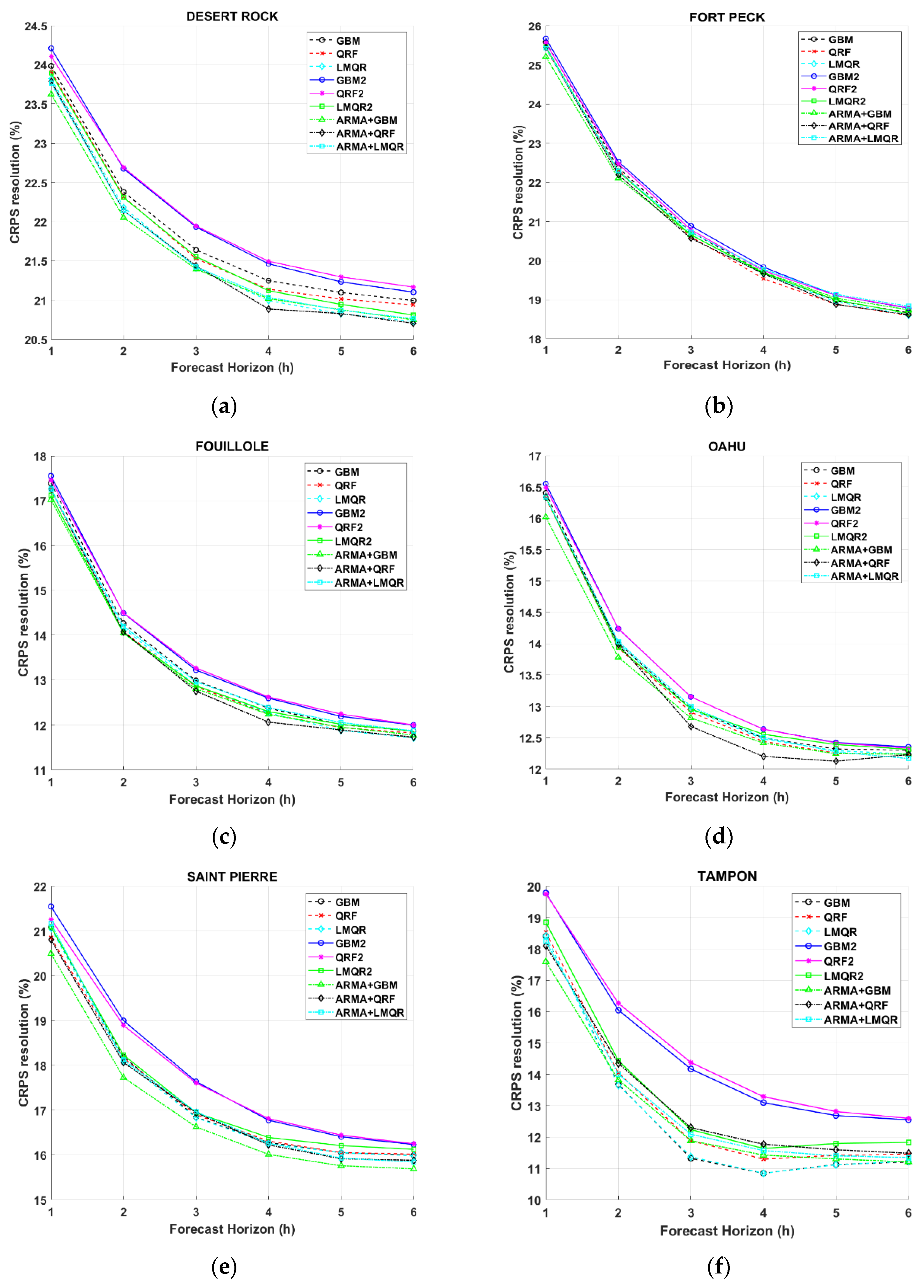
5.1. CRPS and Its Decomposition into Resolution and Reliability

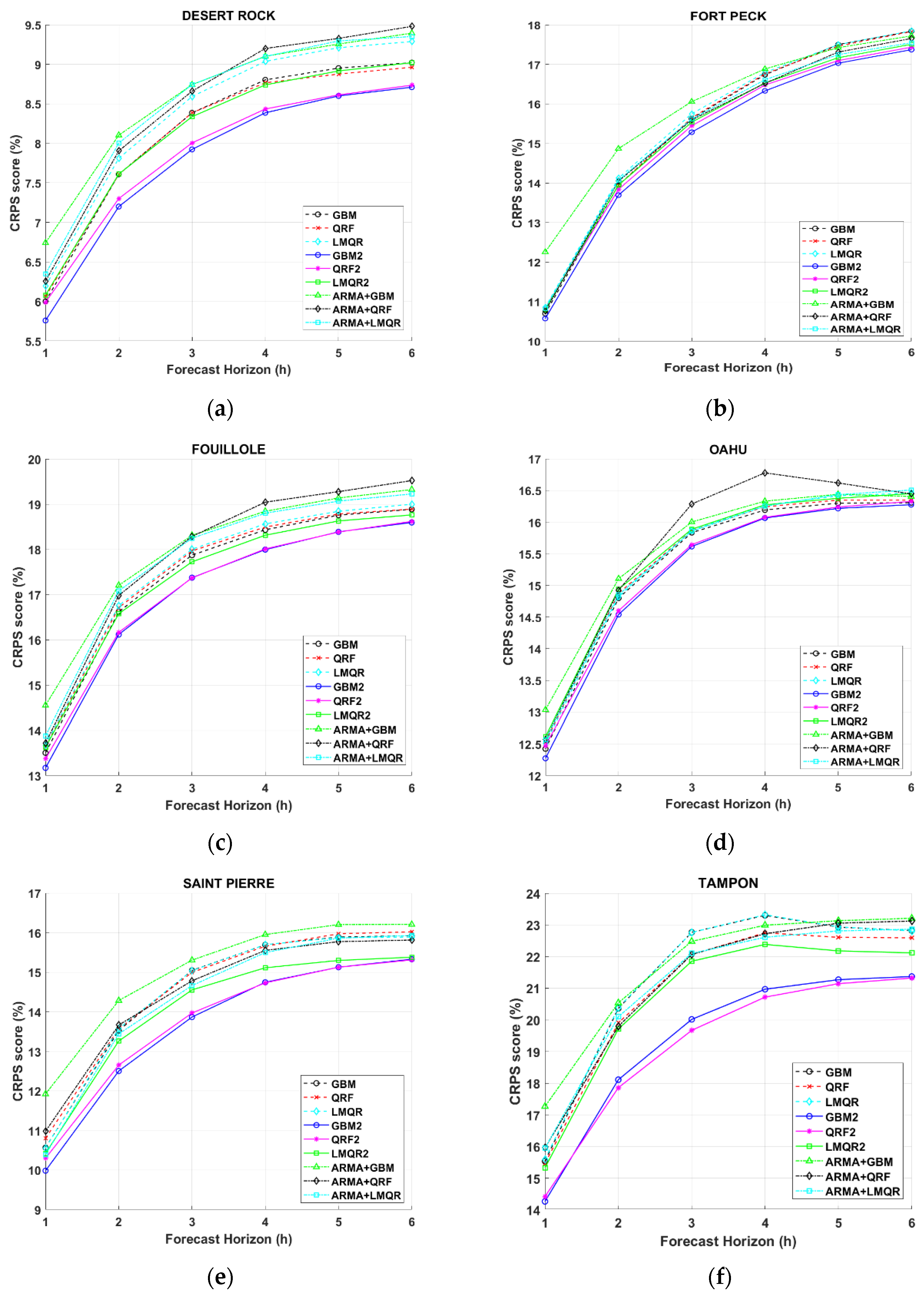
This sub-section provides a detailed insight into the overall accuracy of quantile regression models by plotting the CRPS and its associated decomposition into reliability and resolution. Figure 2 plots the relative CRPS in relation with the forecast horizon for the considered sites, Desert Rock (DR), Fort Peck (FP), Fouillole (FOU), Oahu (OA), Saint Pierre (SP), and Tampon (TA).

As expected, the CRPS of all models increase with the time horizon (in case of CRPS, the lower the better). One also may notice that TA, with more variable sky conditions compared to the other locations, exhibits (as expected) higher CRPS. On the other hand, DR with less cloudy days presents the best forecasting results. Rest of the locations show similar CRPS scores between both TA and DR stations, according to its similar sky condition variability.

As shown in Figure 4, we can easily observe that both variants based on methodology 2 (with and without SZA and HA angles inputs) offer better results than methodology 1 (ARMA model + quantile regression models). DR, FP, FOU, and OA location show the best results when solar angles are used as inputs, while methodology 2 without angles offers better CRPS results than ARMA models. Only in TA and SP we can observe similar results between ARMA models and LMQR, QRF, and GBM. At every location, ARMA + GBM or ARMA + QRF perform the worst probabilistic forecasting. Moreover, the two models based on methodology 2 including solar angles as inputs (GBM2 and QRF2) clearly improve the other models, albeit the discrepancy is less pronounced for FP and OA stations. In terms of CRPS, GBM2, and QRF2 at DR, FOU, SP, and TA locations offer important improvements compared to the rest of the models (around 1% in terms of CRPS score results, see

Table A1. CRPS score and IGN errors for all locations, models, and time horizons tested in this paper. Bold formats point the best models for each station.

Station	Models	CRPS Score (%)						IGN
		T.H. 1 h	T.H. 2 h	T.H. 3 h	T.H. 4 h	T.H. 5 h	T.H. 6 h	T.H. 1 h	T.H. 2 h	T.H. 3 h	T.H. 4 h	T.H. 5 h	T.H. 6 h
Desert Rock	GBM	6.00	7.61	8.39	8.80	8.95	9.02	2.22	2.35	2.39	2.42	2.42	2.42
	QRF	6.06	7.61	8.39	8.77	8.88	8.96	2.22	2.35	2.39	2.41	2.42	2.42
	LMQR	6.20	7.81	8.59	9.04	9.21	9.29	2.27	2.40	2.45	2.47	2.48	2.48
	GBM2	5.76	7.20	7.92	8.39	8.60	8.71	2.19	2.30	2.34	2.38	2.40	2.41
	QRF2	5.99	7.30	8.01	8.43	8.61	8.74	2.15	2.26	2.31	2.34	2.36	2.37
	LMQR2	6.08	7.61	8.34	8.74	8.92	9.02	2.24	2.38	2.42	2.44	2.44	2.45
	ARMA+GBM	6.74	8.10	8.74	9.10	9.26	9.39	2.28	2.39	2.43	2.46	2.45	2.46
	ARMA+QRF	6.26	7.91	8.66	9.20	9.33	9.48	2.29	2.40	2.43	2.46	2.47	2.47
	ARMA+LMQR	6.35	8.00	8.74	9.10	9.30	9.35	2.30	2.41	2.44	2.46	2.46	2.47
Fort Peck	GBM	10.70	13.95	15.63	16.74	17.50	17.84	2.46	2.56	2.60	2.62	2.63	2.64
	QRF	10.83	13.94	15.65	16.76	17.46	17.83	2.46	2.56	2.60	2.62	2.63	2.63
	LMQR	10.86	14.12	15.75	16.79	17.50	17.85	2.47	2.57	2.61	2.63	2.63	2.64
	GBM2	10.57	13.69	15.29	16.33	17.03	17.37	2.45	2.55	2.60	2.62	2.63	2.64
	QRF2	10.83	13.84	15.45	16.48	17.10	17.43	2.42	2.53	2.57	2.59	2.61	2.62
	LMQR2	10.79	13.95	15.54	16.53	17.17	17.51	2.46	2.57	2.61	2.63	2.64	2.65
	ARMA+GBM	12.26	14.87	16.06	16.88	17.42	17.72	2.53	2.59	2.61	2.63	2.63	2.64
	ARMA+QRF	10.76	14.05	15.60	16.52	17.31	17.65	2.48	2.57	2.61	2.62	2.64	2.64
	ARMA+LMQR	10.83	14.07	15.62	16.61	17.25	17.55	2.47	2.57	2.59	2.62	2.62	2.63
Fouillole	GBM	13.50	16.62	17.87	18.43	18.76	18.89	2.72	2.79	2.81	2.82	2.82	2.81
	QRF	13.64	16.71	17.97	18.49	18.78	18.89	2.72	2.79	2.81	2.82	2.82	2.82
	LMQR	13.67	16.76	18.00	18.56	18.84	19.00	2.72	2.79	2.81	2.83	2.83	2.83
	GBM2	13.17	16.12	17.37	17.99	18.39	18.59	2.71	2.78	2.80	2.81	2.81	2.81
	QRF2	13.37	16.16	17.37	18.01	18.38	18.62	2.69	2.75	2.78	2.79	2.80	2.80
	LMQR2	13.63	16.58	17.72	18.31	18.63	18.76	2.72	2.78	2.80	2.81	2.81	2.81
	ARMA + GBM	14.55	17.20	18.31	18.84	19.14	19.32	2.76	2.81	2.82	2.83	2.83	2.84
	ARMA + QRF	13.72	16.98	18.29	19.04	19.28	19.52	2.74	2.80	2.82	2.83	2.83	2.84
	ARMA + LMQR	13.88	17.08	18.25	18.80	19.07	19.23	2.73	2.80	2.81	2.82	2.82	2.83
Oahu	GBM	12.42	14.80	15.83	16.19	16.30	16.30	2.67	2.74	2.75	2.77	2.76	2.76
	QRF	12.53	14.88	15.87	16.24	16.35	16.35	2.67	2.74	2.75	2.76	2.77	2.76
	LMQR	12.51	14.82	15.87	16.27	16.42	16.46	2.68	2.74	2.76	2.77	2.77	2.77
	GBM2	12.27	14.54	15.61	16.06	16.22	16.28	2.62	2.69	2.71	2.71	2.72	2.72
	QRF2	12.47	14.60	15.64	16.08	16.24	16.33	2.60	2.66	2.69	2.70	2.71	2.71
	LMQR2	12.61	14.94	15.89	16.27	16.38	16.45	2.64	2.69	2.71	2.72	2.72	2.72
	ARMA + GBM	13.04	15.11	16.00	16.33	16.44	16.40	2.70	2.75	2.76	2.77	2.77	2.77
	ARMA + QRF	12.57	14.93	16.29	16.78	16.62	16.45	2.68	2.75	2.77	2.79	2.79	2.77
	ARMA + LMQR	12.56	14.85	15.86	16.25	16.44	16.51	2.68	2.74	2.75	2.76	2.77	2.77
Saint Pierre	GBM	10.57	13.53	15.05	15.69	15.89	15.92	2.67	2.79	2.83	2.84	2.84	2.84
	QRF	10.80	13.57	15.00	15.66	15.97	16.02	2.71	2.80	2.84	2.84	2.85	2.84
	LMQR	10.56	13.58	15.04	15.70	15.87	15.88	2.71	2.84	2.86	2.87	2.87	2.87
	GBM2	9.98	12.50	13.87	14.74	15.13	15.33	2.62	2.74	2.80	2.82	2.82	2.83
	QRF2	10.30	12.65	13.97	14.73	15.12	15.31	2.66	2.75	2.79	2.81	2.82	2.81
	LMQR2	10.42	13.26	14.55	15.11	15.30	15.38	2.71	2.83	2.86	2.86	2.86	2.86
	ARMA + GBM	11.92	14.28	15.30	15.95	16.20	16.21	2.73	2.82	2.87	2.88	2.88	2.90
	ARMA + QRF	10.98	13.66	14.78	15.55	15.77	15.81	2.70	2.80	2.86	2.87	2.88	2.89
	ARMA + LMQR	10.39	13.44	14.66	15.50	15.86	15.93	2.67	2.81	2.85	2.87	2.88	2.88
Tampon	GBM	15.54	20.37	22.77	23.30	22.93	22.82	2.70	2.79	2.82	2.83	2.82	2.83
	QRF	15.47	19.90	22.07	22.75	22.61	22.59	2.68	2.77	2.81	2.82	2.82	2.82
	LMQR	15.59	20.39	22.76	23.32	22.94	22.81	2.70	2.81	2.83	2.83	2.84	2.83
	GBM2	14.26	18.11	20.01	20.97	21.27	21.37	2.66	2.77	2.79	2.81	2.82	2.82
	QRF2	14.42	17.86	19.67	20.72	21.14	21.32	2.61	2.69	2.73	2.75	2.76	2.77
	LMQR2	15.33	19.71	21.85	22.38	22.18	22.12	2.71	2.80	2.83	2.83	2.83	2.83
	ARMA + GBM	17.26	20.54	22.48	22.99	23.13	23.21	2.78	2.83	2.84	2.85	2.85	2.85
	ARMA + QRF	15.96	19.79	22.07	22.72	23.05	23.12	2.74	2.80	2.83	2.84	2.84	2.84
	ARMA + LMQR	15.95	20.10	22.10	22.61	22.81	22.87	2.73	2.80	2.82	2.83	2.83	2.83

in the Appendix C).

Regarding only methodology 2, one may notice also that LMQR2 based on a linear regression does not perform as well as its nonlinear counterparts (GBM2 and QRF2) but SZA and HA angles improve the results compared with past data only (LMQR). LMQR model offers the worst results between methodology 2 models. Figure A2 also confirms that among the group of methods of methodology 1, ARMA + LMQR method exhibits slightly better performance than the other two.

Figure 5 shows the resolution part of the CRPS. As for CRPS score, increasing time horizon forecasting quantile regression distributions present lack of resolution (for the resolution, the lower values indicate a worse resolution). Regarding resolution, the observations made with the CRPS score still hold. In particular, the GBM2 and QRF2 models, including solar angle inputs, give us better resolution in particularly for the site of TA, SP, FOU, and DR stations. In addition, one may notice that GBM2 and QRF2 models have roughly the same resolution. We can also notice again that both variants of methodology 2 outperform methodology 1 models in FR, OA, and SP stations. FP and FOU reproduce similar results between methodology 2 without angles and ARMA model, while LMQR and GGM obtained the worst results for TA.

Interestingly, Figure 5 shows that ARMA+LMQR gives the best results of methodology 1 and ARMA+GBM and ARMA+QRF obtain the worst results of all models. For methodology 2, as we observed in CRPS score, resolution leads us to conclude that GBM2 and QRF2 give the best results for all locations. Indeed, using solar geometric angles in addition to the past values of the GHI improves forecasting performance.

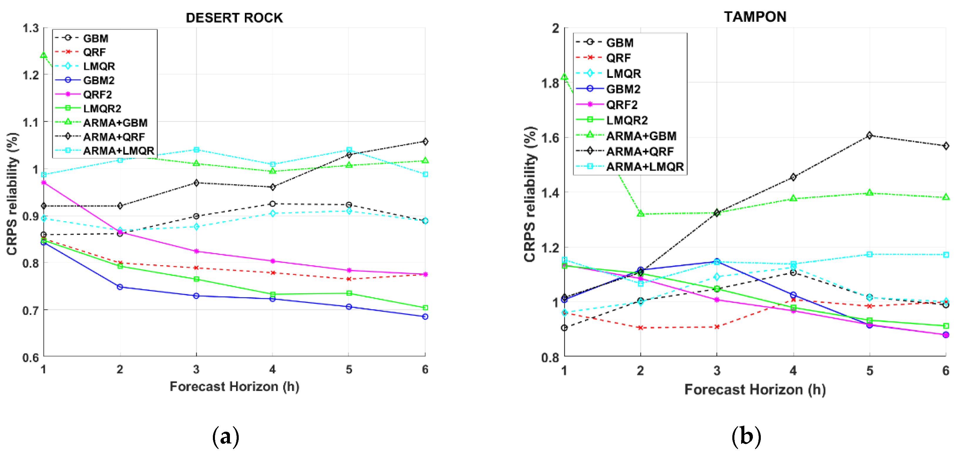
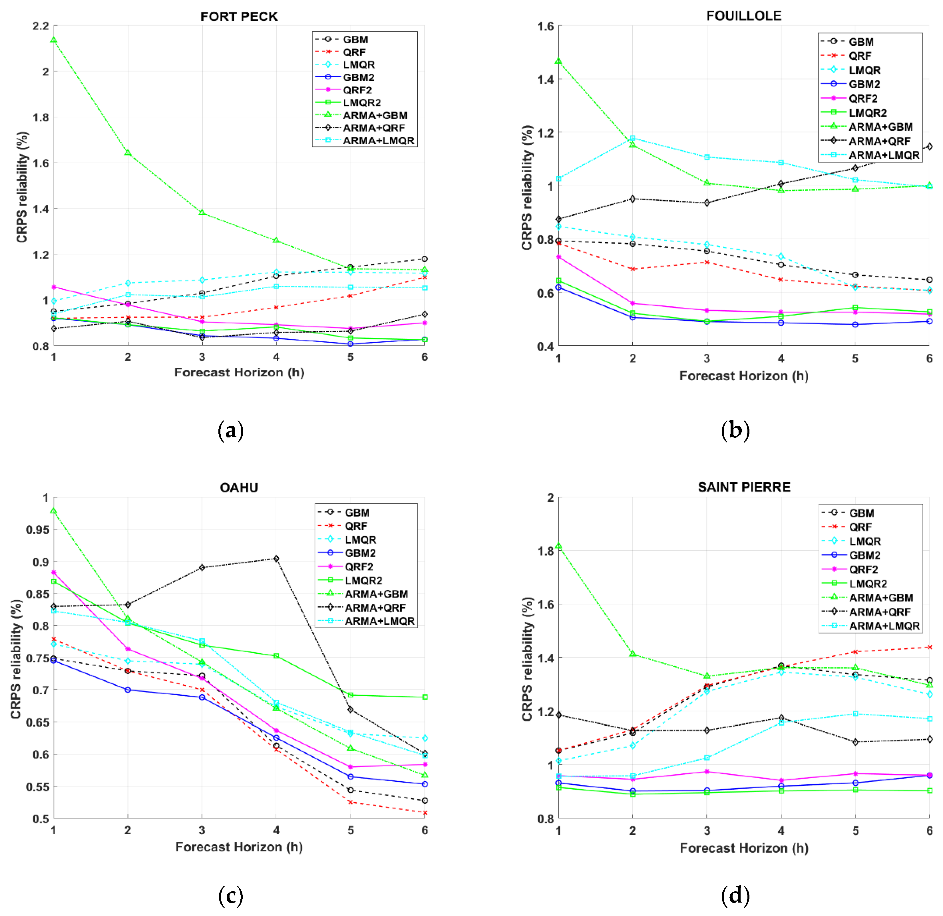
Figure 6 plots the reliability term of the CRPS. Surprisingly, the reliability does not show a clear tendency while time horizon increases. The values of the reliability are approximately ten times smaller than the values of the resolution. In other words, reliability only forms a small part of the CRPS, and the higher quality of the probabilistic forecasts originates mainly from the resolution attribute. Figure 6 shows CRPS reliability for DR and TA locations, which experience the most extreme GHI variability. The Figure A1 in the Appendix A shows the results for the rest of the locations. It appears that GBM2 method leads to a more reliable quantile regression than QRF2, more specifically in DR. In addition, GBM2, QRF2, GBM, and QRF (methodology 2) give better results in terms of reliability for all location than the rest of the models. Particularly for TA station, QRF offers the best results, although for higher time horizons QRF2 and GBM2 obtain better results. This finding may encourage the decomposition of the CRPS into reliability and resolution as it provides more information regarding the performances of the models. This may help the user to objectively select more reliable models. Results also establish that ARMA models with methodology 1 obtained worse results in general.

The CRPS decomposition gives enough information to see that, in general, methodology 2 with and without solar angles obtain better results. Comparing the two methodology 2 variants, the adding of the two-extra solar geometric variables improves the forecasting performance as demonstrated by the better performance of the GBM2 and QRF2. For DR, TA, and SP locations, improvements obtained with methodology 2 with solar angles are considered significant.

5.2. Score Metrics Discussion

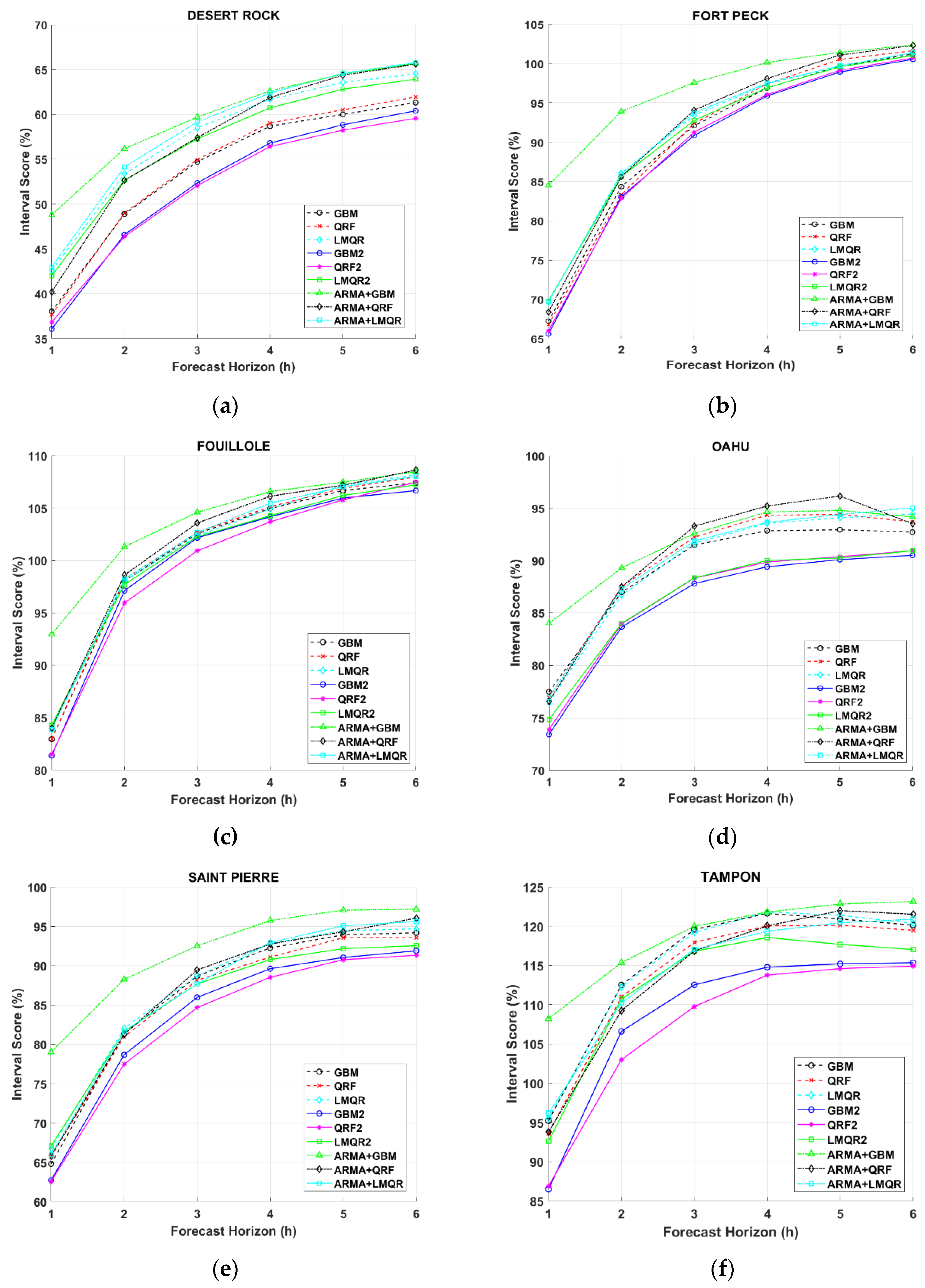
In addition to the CRPS and its decomposition, we studied different scores to obtain more information about quantile regression performance at every location. In this case, we focused the study on interval score (IS), quantile score (QS), and LogScore.

As shown in Equation (25), IS penalizes forecasts outside the interval according to the value of α. For this paper, we calculate IS for the 80% central prediction interval. Figure 7 clearly shows an improvement in QRF2 and GBM2. These two models obtain better results at all locations, especially in DR, OA, SP, and TA. According to IS results, QRF2 model obtains better quantile regression forecasting for all stations and time horizons. Models obtained with methodology 2 and solar angles clearly outperform the rest of the models. In this case, at DR, FP, FOU, OA, and SP forecasted distribution obtained directly with past data clearly outperforms ARMA models. Only at TA measurement station, we can observe similar results between ARMA + LMQR and the rest of the models.

DR, OA, SP, and TP results obtained with QRF2 and GBM2 offer more important improvements compared to the rest of the models. ARMA + GBM seem to give the worst results at all locations. The rest of methodology 1 models present similar results between them. While comparing only methodology 2, the variant with solar angles outperforms regression models with only past measurement inputs.

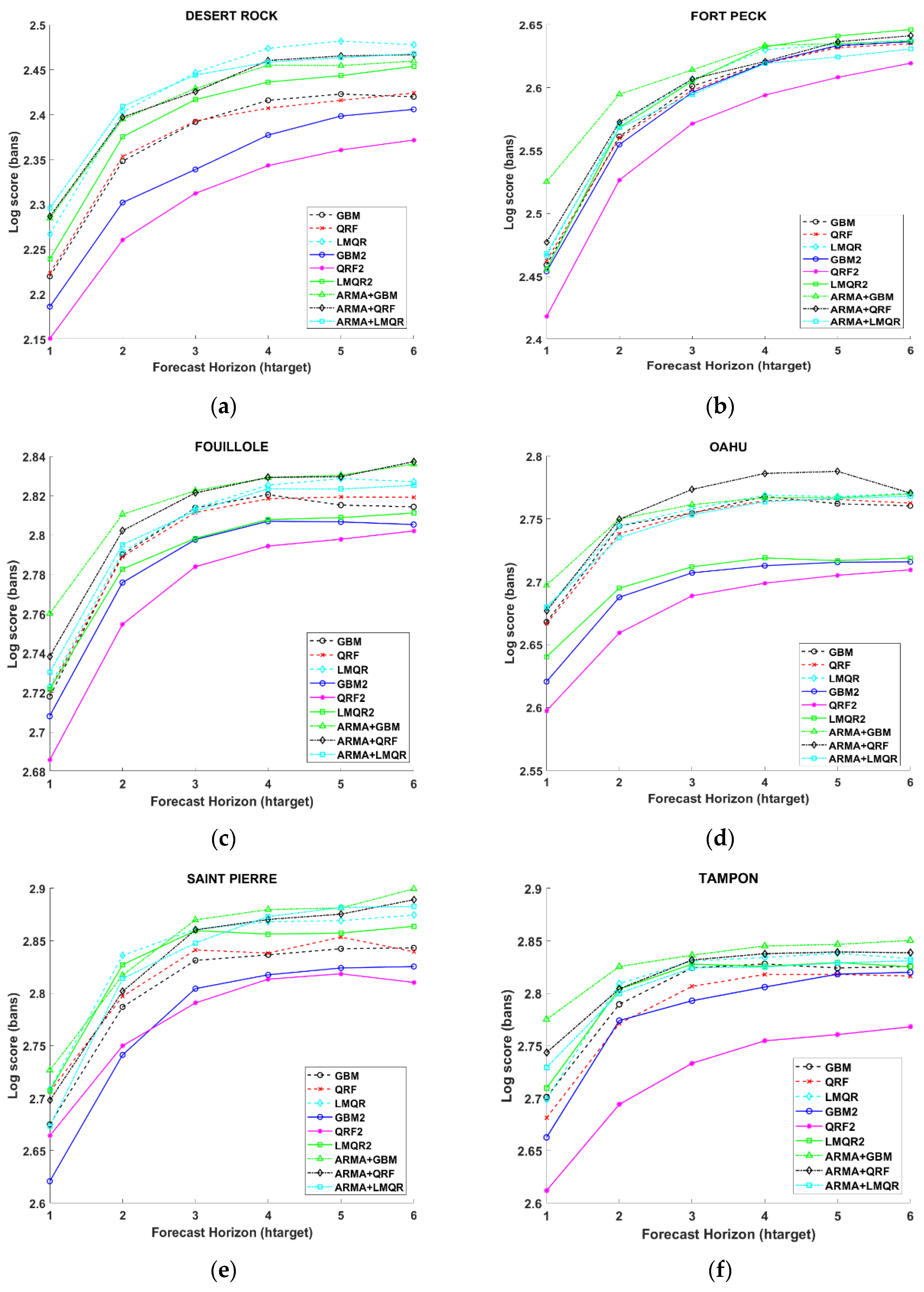
Figure 8 plots the LogScore or ignorance (IGN) for all locations. As explained before, IGN lower values correspond to a better forecasting performance. In our case, IGN figures confirm that methodology 2 using solar geometric angles obtains the best results (specifically QRF2 and GBM2). It is also easy to see that ARMA models are worse than methodology 2 for all the locations. Indeed, the information obtained from CRPS decomposition and IGN could give the user more confidence in selecting QRF2 model as the best one (almost 2% of improvements at TA, SP, OA, and DR and around 1% for FP and FOU). This model presents a large improvement at every location compared to the rest of the models, see Table A1. Again, it is easy to observe that methodology 2 models improve ARMA models in general. ARMA + QRF and ARMA + GBM are always the worst models at all locations and only ARMA + LMQR obtains similar results as LMQR, GBM, and QRF for TA, OA, FOU, and FP.

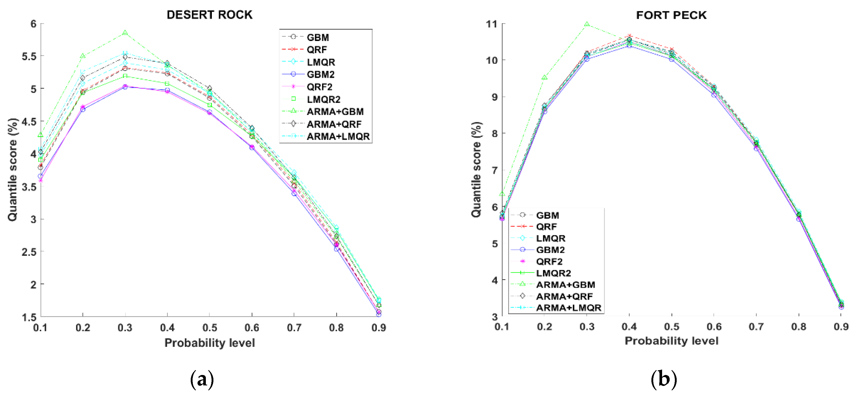
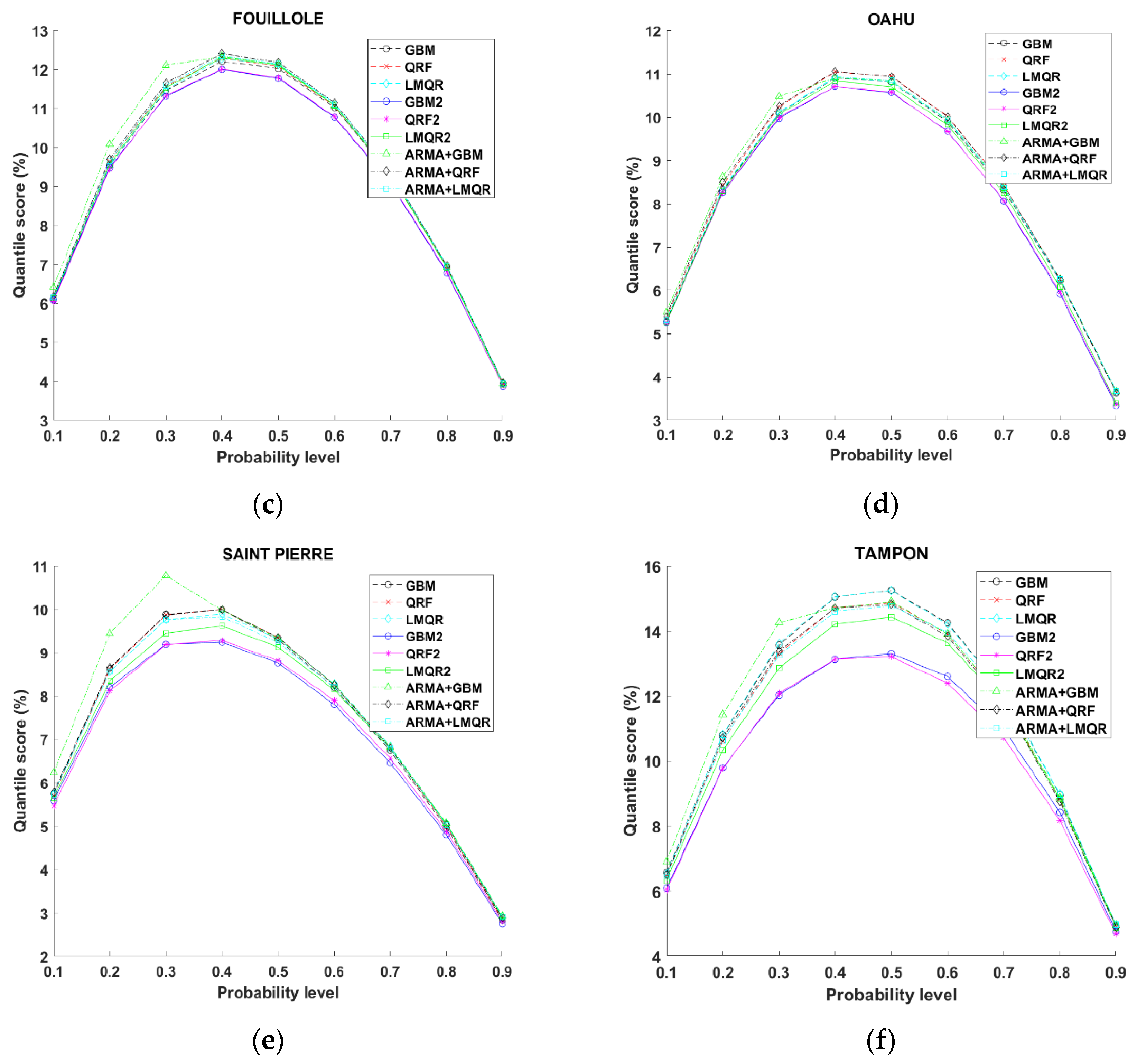
Finally, we used the quantile score (QS) to study all the models (we should recall that this metric is negatively oriented). QS allows to obtain detailed information about the forecast quality at specific quantiles. Figure 9 plots the quantile score in relation to the probability levels ranging from 0.1 to 0.9. As we observed with the previous scores, methodology 2 obtains clearly better results for all stations and time horizons. Methodology 1 gives us worse results for all quantiles compared with QRF2 and GBM2 (more accused in TA, SP and DR stations). In case of TA station, these two methods give clearer improvements. TA shows a symmetric QS pattern, which means that the highest and lowest quantiles present similar forecasting results. On the other hand, at DR location the lowest quantiles present the worst results and an asymmetric pattern. The rest of the stations show results between these two extreme cases. This is possibly due to lower variability observed at DR and the rest of locations compared to TA (i.e., high occurrences of clear skies).

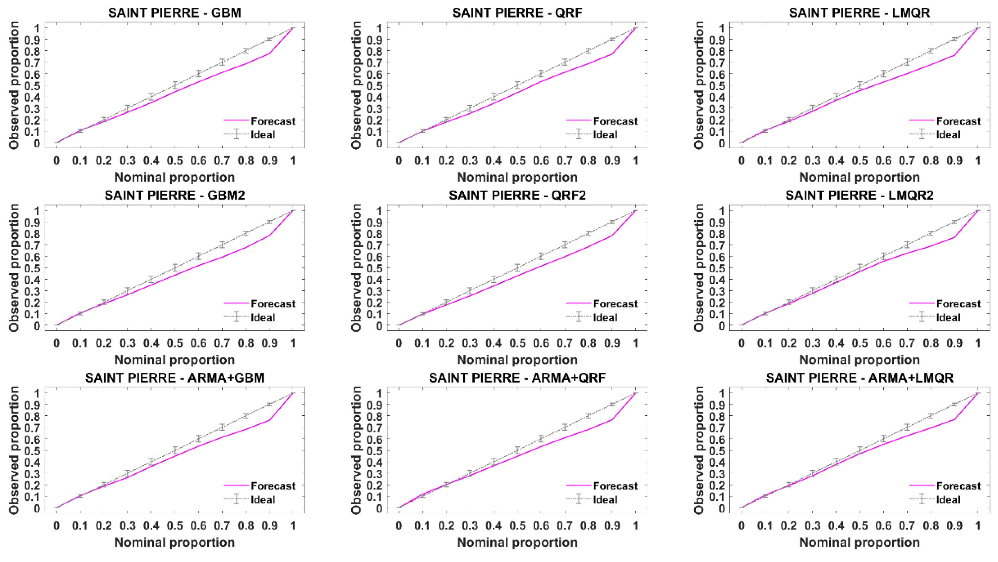
5.3. Application of the Diagnostic Tools

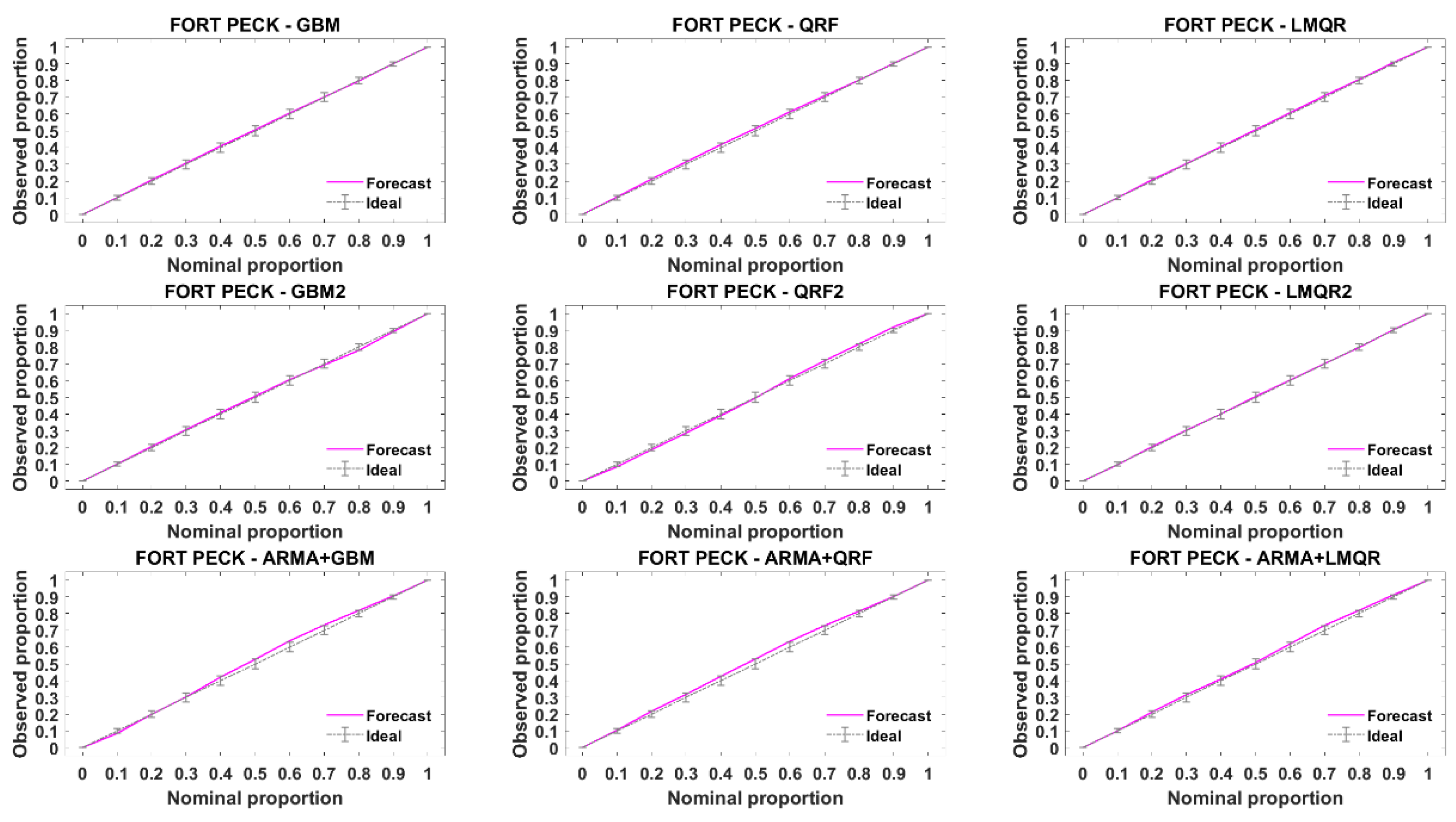
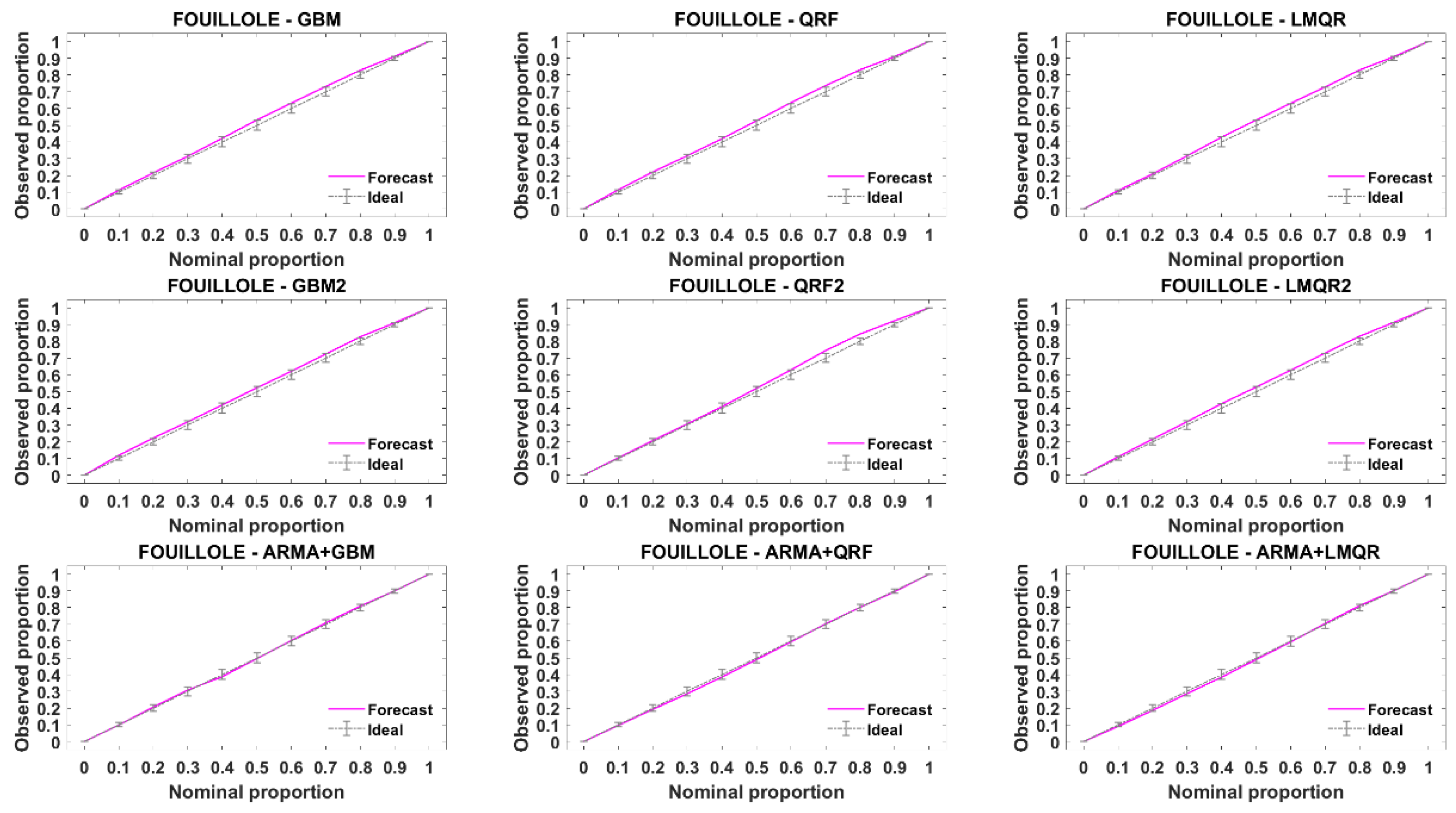
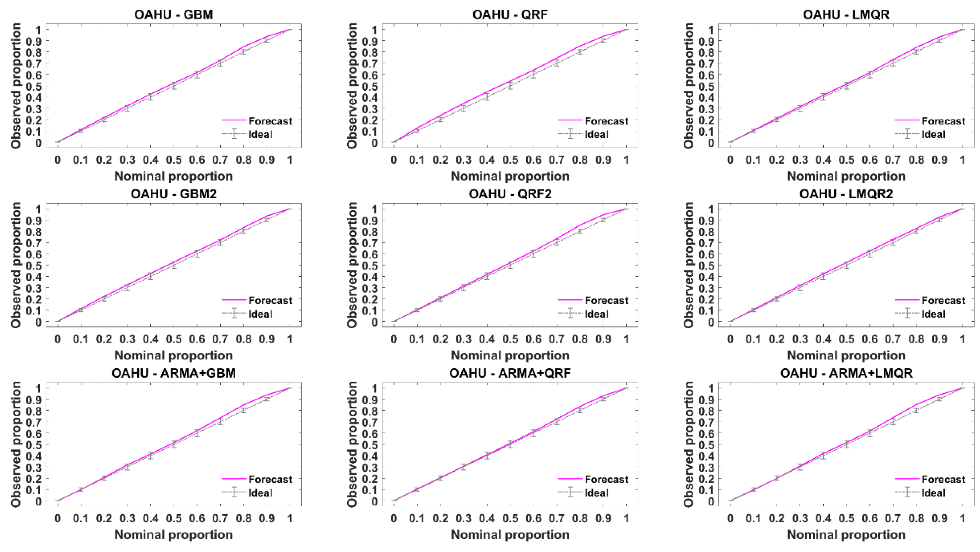
As mentioned above, these graphical diagnostic tools allow assessing the reliability for a probabilistic forecasting, but hardly help to select between a set of regression models. In this paper we only show the results obtained with the reliability diagram. Selecting the best forecasting approach using this diagnosis tool leads us to a less clear picture, but we can obtain information about reliability of selected models. First, to provide synthetic results, it must be noted that the reliability diagrams are averaged for all the forecasting time horizons.

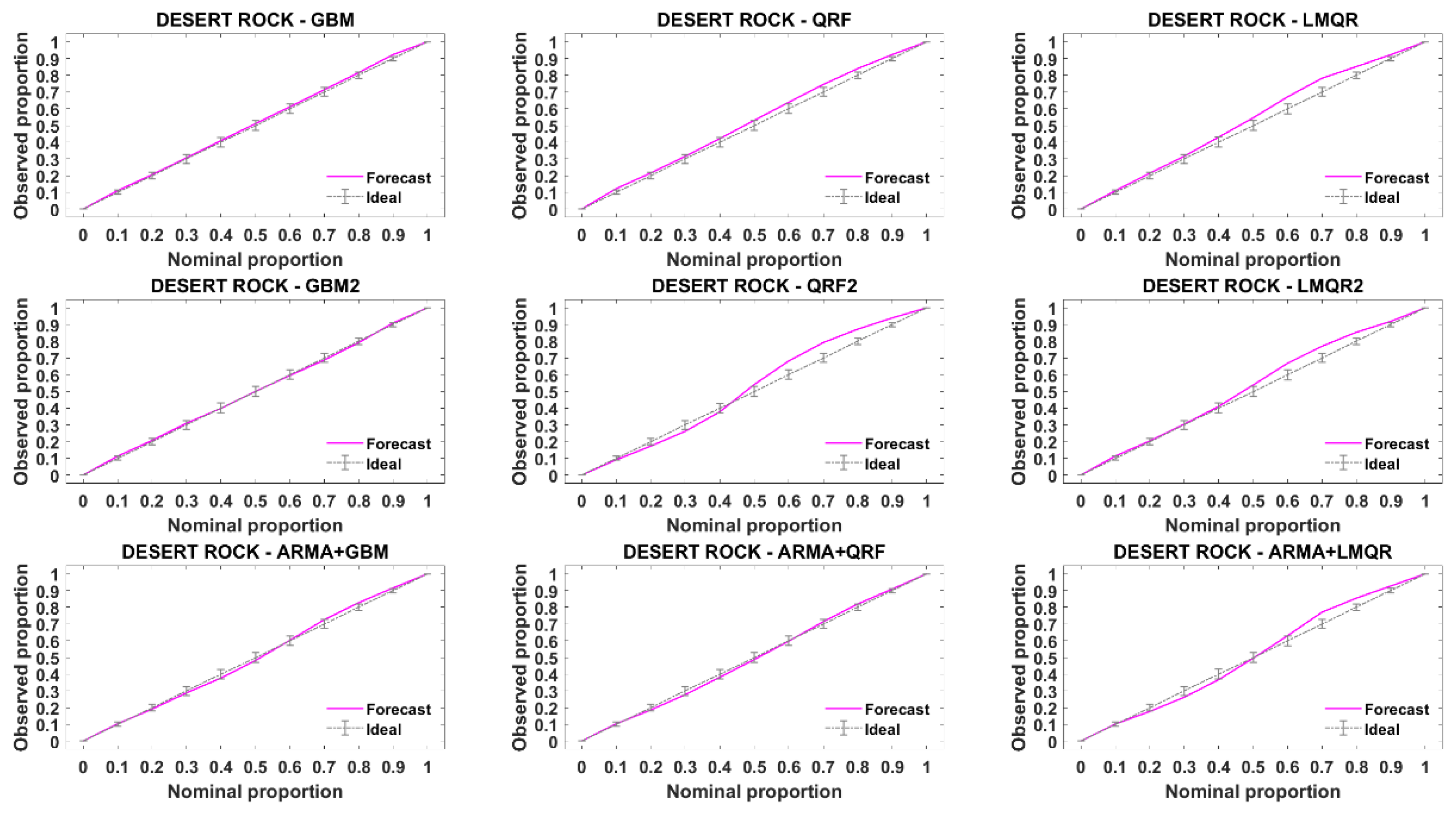
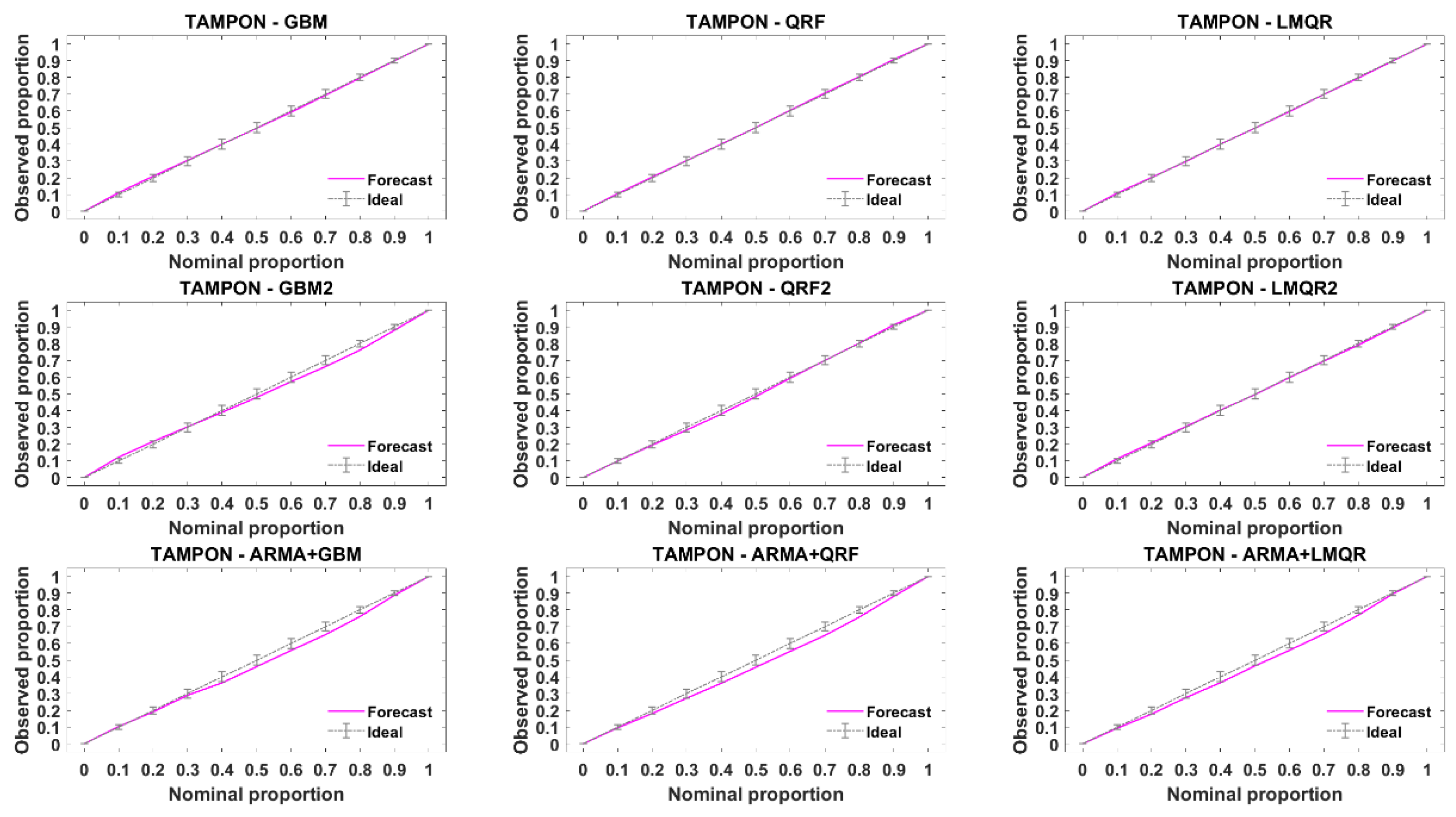
Figure 10 and Figure 11 provide the reliability diagrams for DR and TA stations, reliability diagrams for the rest of the stations can be found in Appendix B. The 1:1 line represents a perfectly reliable forecasting. When the line corresponding to a particular model lies under the ideal line, the model is overconfident. On the contrary, when the model is above the ideal line, the model is underconfident. According to these figures, slight departures from the ideal line are noted for all the models. We can only point that QRF2 obtains slightly worse results at DR station than the rest of the models and that solar geometric angles do not improve reliability compared to the rest of the models.

One may state that, when discrepancy from perfect reliability is rather small (as it is the case), it may be difficult to select the best model with the help of this graphical display. Nevertheless, this graphical display may be interesting to pinpoint non-reliable quantile regression and it is better relying on quantitative values, because of the CRPS decomposition in resolution and reliability. Compared to ARMA models in methodology 1, one cannot notice any important difference in reliability diagrams.

6. Conclusions and Perspectives

In this paper, two different methodologies to estimate solar probabilistic forecasts were appraised according to a detailed verification framework. Different metrics previously tested by the solar community were used to study both methodologies. Six sites with very different weather conditions were chosen to illustrate the comparisons.

The methodology 1, which has already been extensively studied in a previous work, uses a point forecast (ARMA) as input for the quantile regression models. The new methodology 2 uses directly past solar radiation data as inputs for the quantile regression models. For this second approach, we also proposed two variants depending on the input data. The first one only uses past data as inputs and the second one adds solar geometric angles (SZA and HA). In order to establish a proper comparison between all models, methodology 1 models were also calculated with the set of metrics proposed in [30].

The results obtained in this work may encourage the user to rely on the CRPS decomposition and different metric scores to get a detailed picture of the forecasting performance of competing models, as pointed by Lauret et al. (2019) [30]. As shown above, the CRPS decomposition gives important information to highlight that methodology 2 clearly shows better performances than methodology 1. While interval and LogScore are the metrics which clearly point QRF2 as the best performer. Furthermore, these metrics also show that all models obtained with methodology 2, both with and without solar geometric angles as inputs, outperform the results obtained with ARMA model combined with quantile regression methods. Moreover, it was clearly demonstrated that the adding of the geometric solar variables, named solar zenith angle and hour angle, have a clear impact on the forecasting accuracy of the probabilistic models.

Also, it is shown that care must be taken in the analysis based on graphical displays like reliability diagram. The graphical analysis of reliability can help understand and confirm the good forecasting performance of the selected model. The results obtained for the different sites and models considered in this paper show that the QRF2 model, which has past solar data and solar angle as inputs, provides the best forecasting skills.

Future work will be focused on decision-making metrics. Indeed, these kinds of metrics are based on the study of the cost and losses that a certain event causes. In this new paper we can compare, at least, the Brier Score, the reliability curve, or the relative operating characteristic (ROC) to assess the value of different probabilistic solar forecasts. Also, we plan to use exogenous inputs, as day-ahead NWP forecasts to increase the performance of the models.