
Endogenous Approach of a Frequency-Constrained Unit Commitment in Islanded Microgrid Systems


Abstract
:1. Introduction
2. UC and Dynamic Models
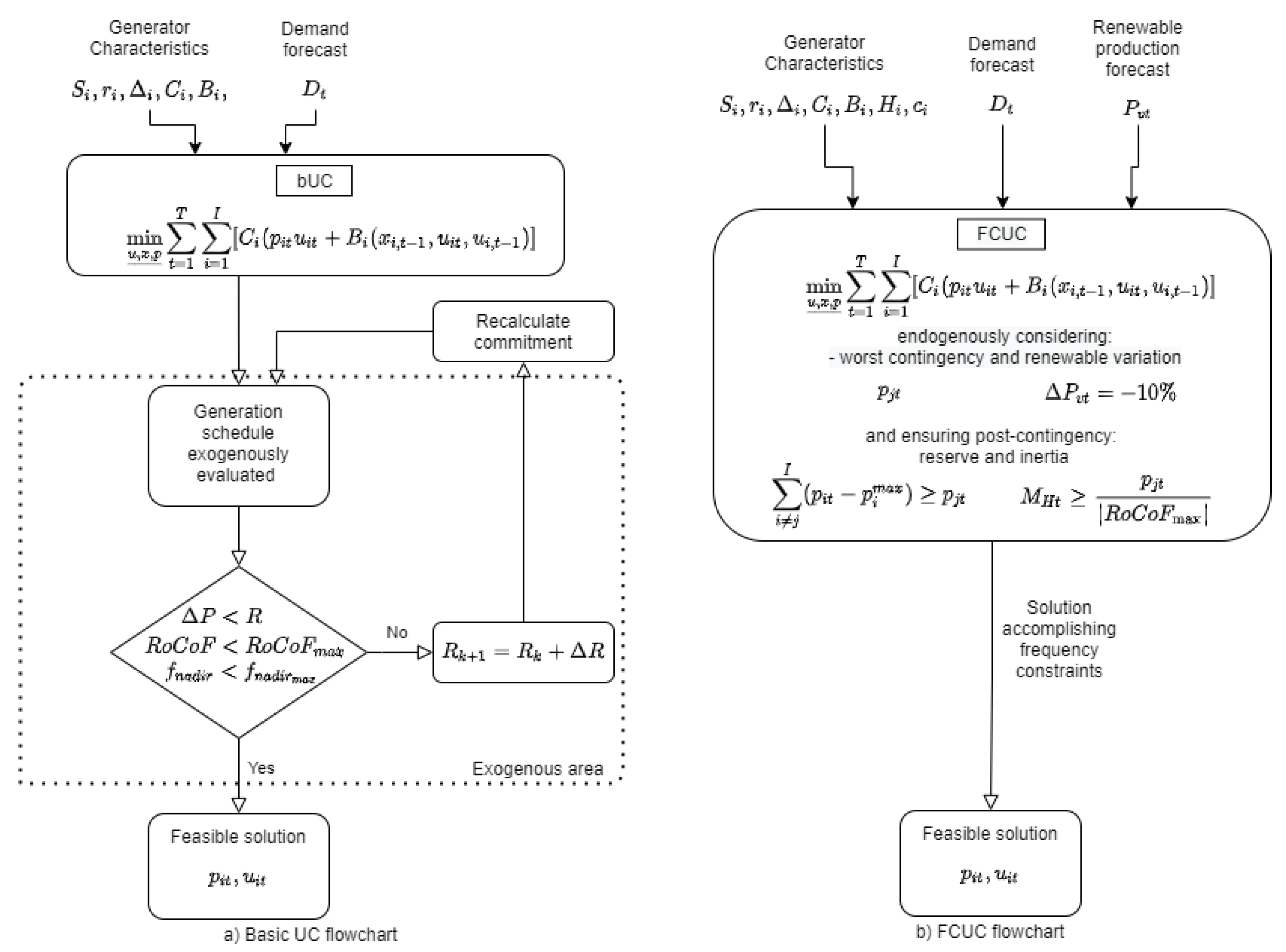
2.1. UC with Exogenous Frequency Constraints, bUC Formulation
- i is the index for the number of units (i = 1, ..., I);
- t is the index for time or nb of hours (t = 0, ..., T);
- is a binary variable defining if the unit i is committed or not at time t;
- is the power generated by unit i at time t;
- is the fuel cost of unit i at power i at time t;
- is the start-up cost;
- is the state variable denoting the time lenth a unit has been up or down.
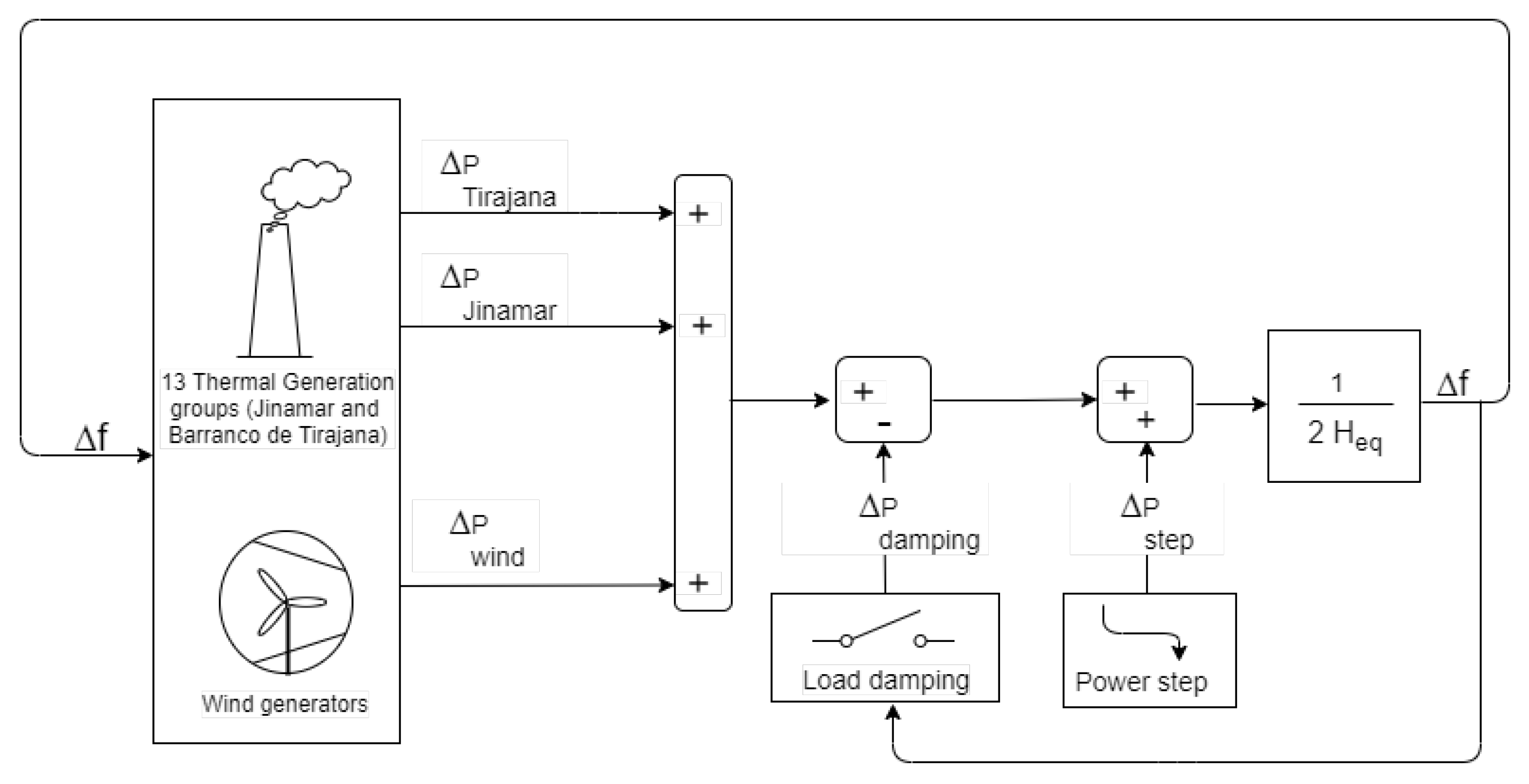
2.2. Frequency Response of Power Sources
Dynamic Models
2.3. UC with Endogenous Frequency Constraints
2.3.1. Dynamic Reserve Allocation
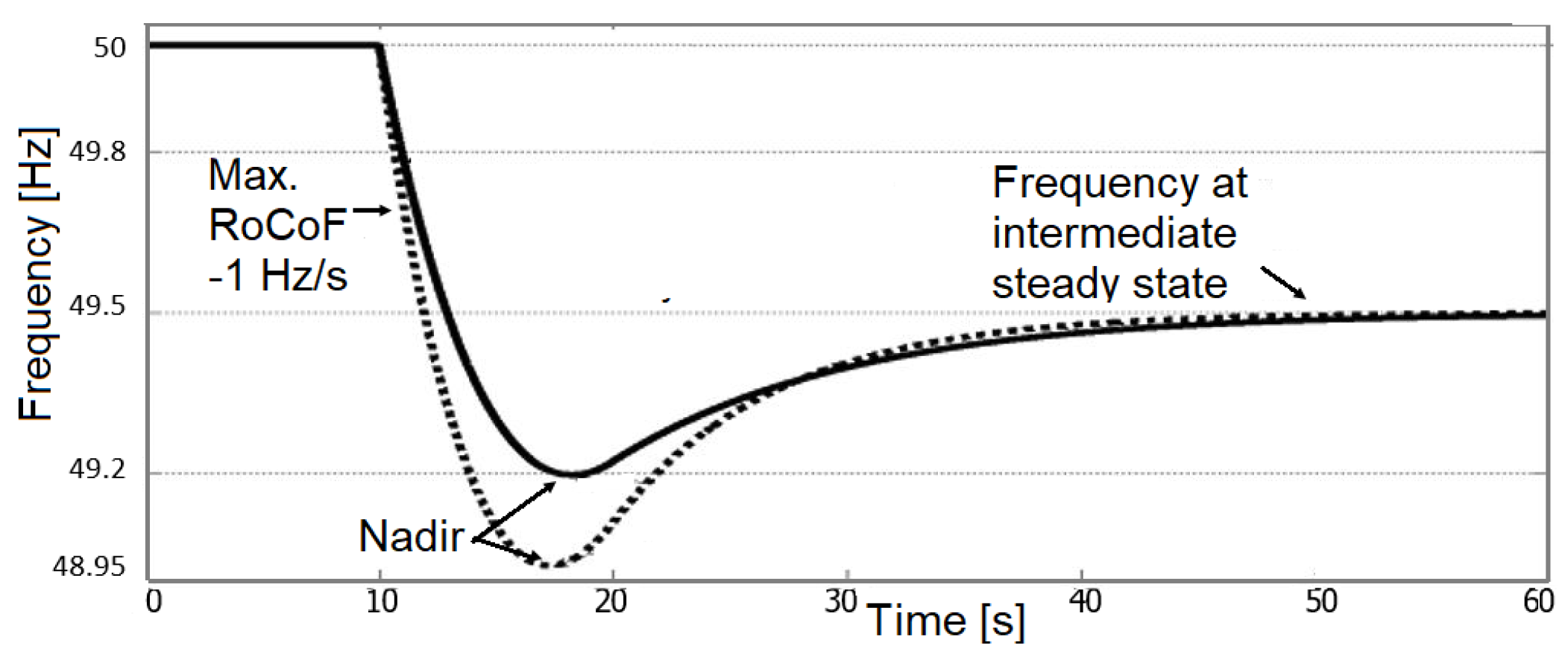
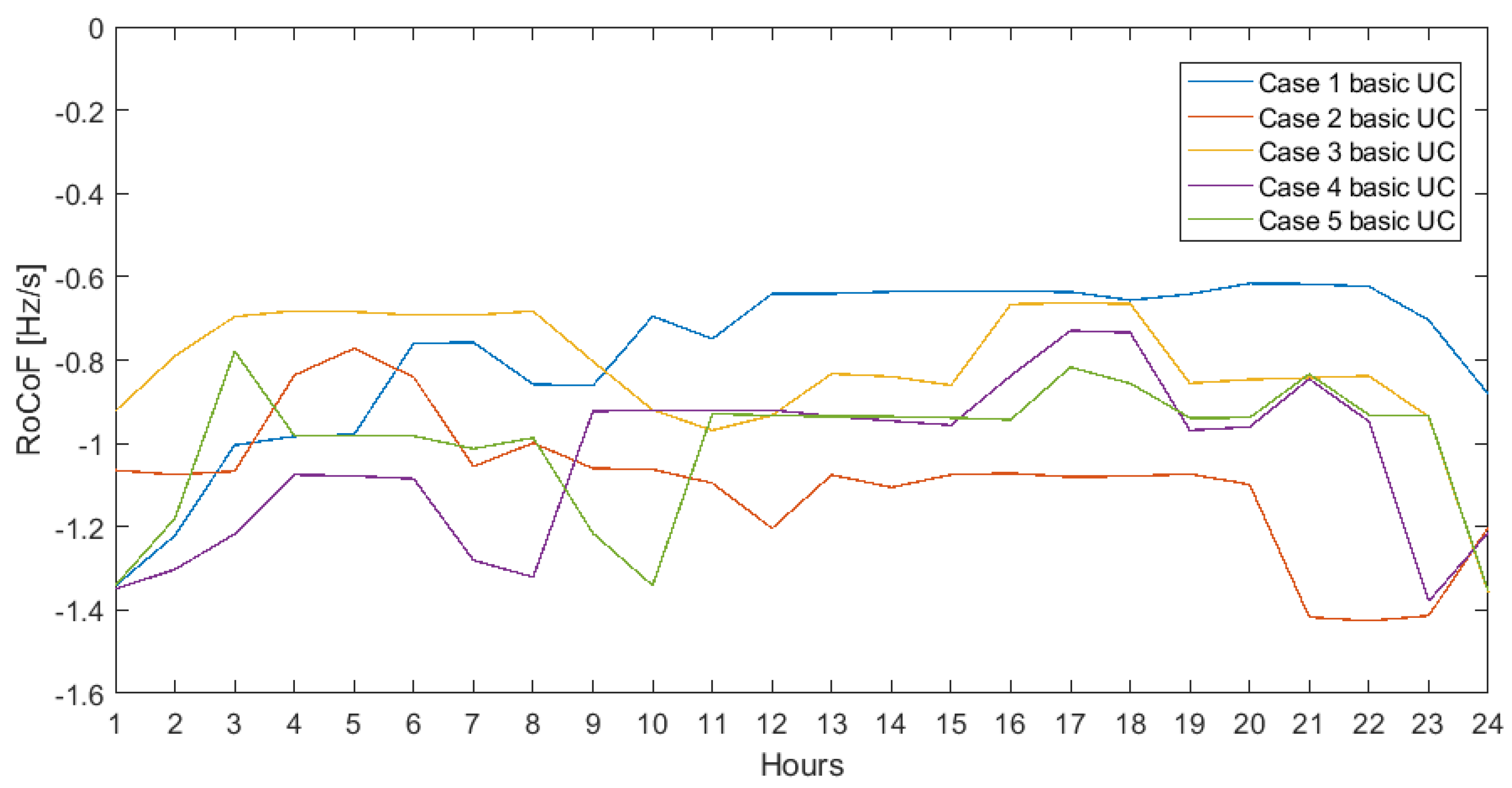
2.3.2. Rate of Change of Frequency
2.3.3. Nadir Frequency
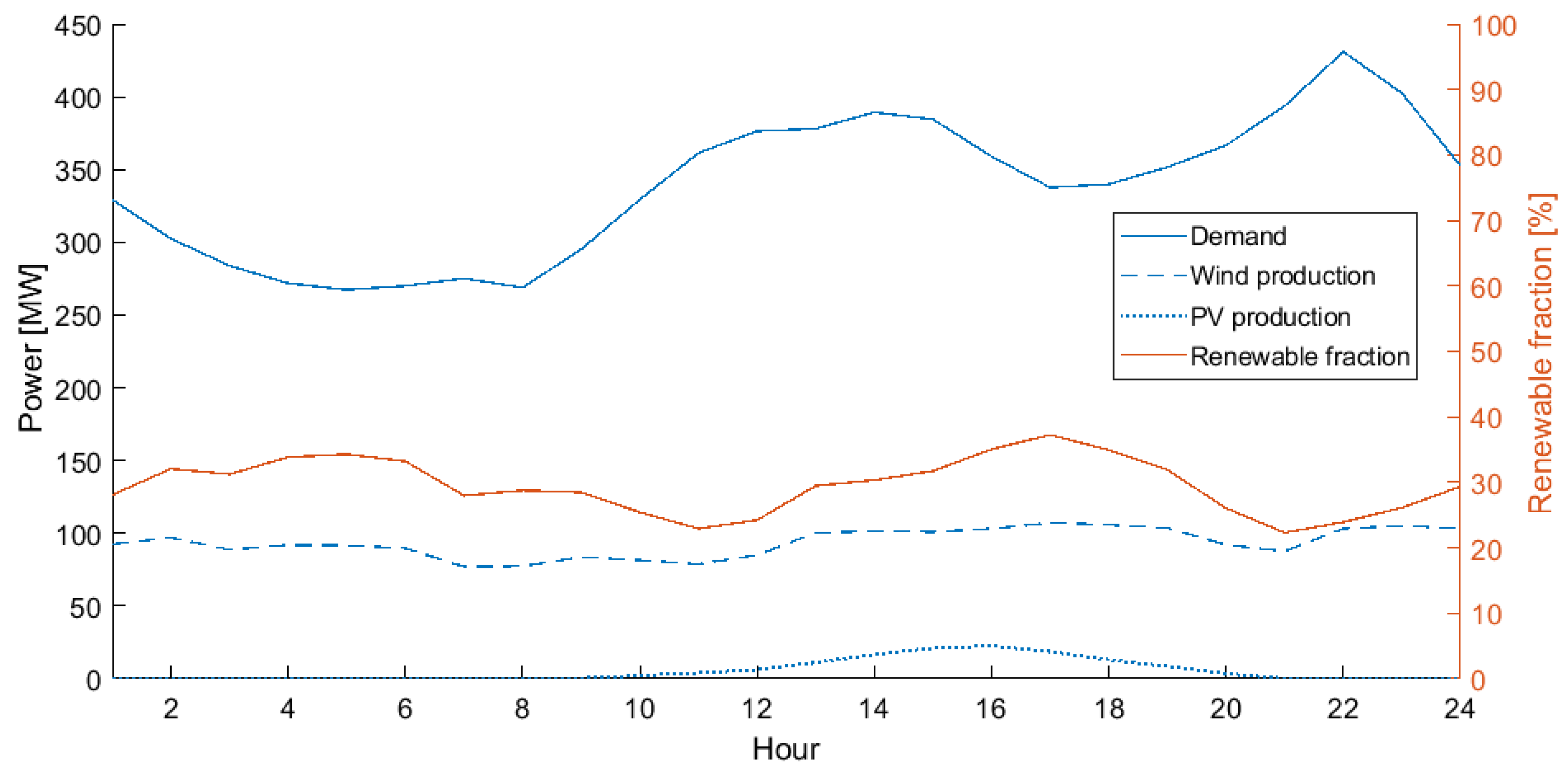
3. Electrical Generation System of Island of Gran Canaria
4. Results
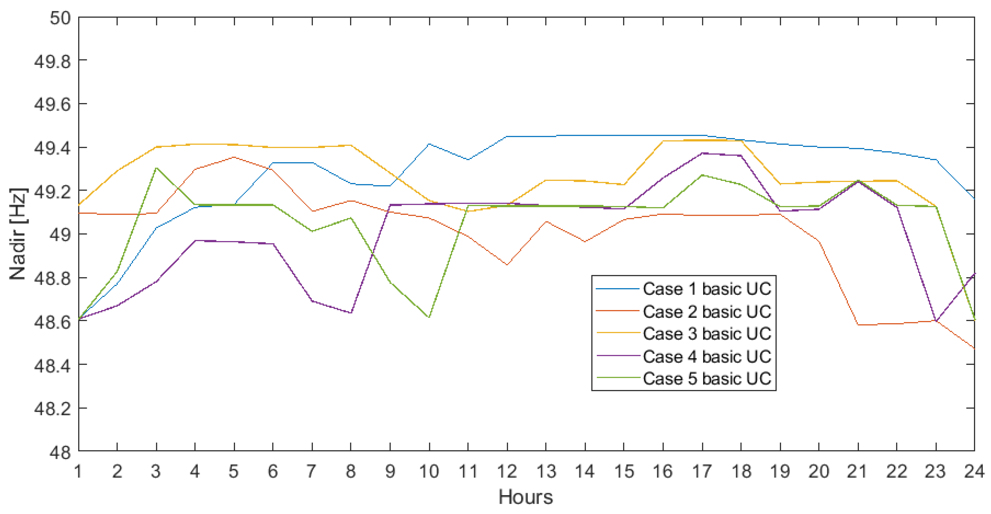
4.1. Basic Unit Commitment
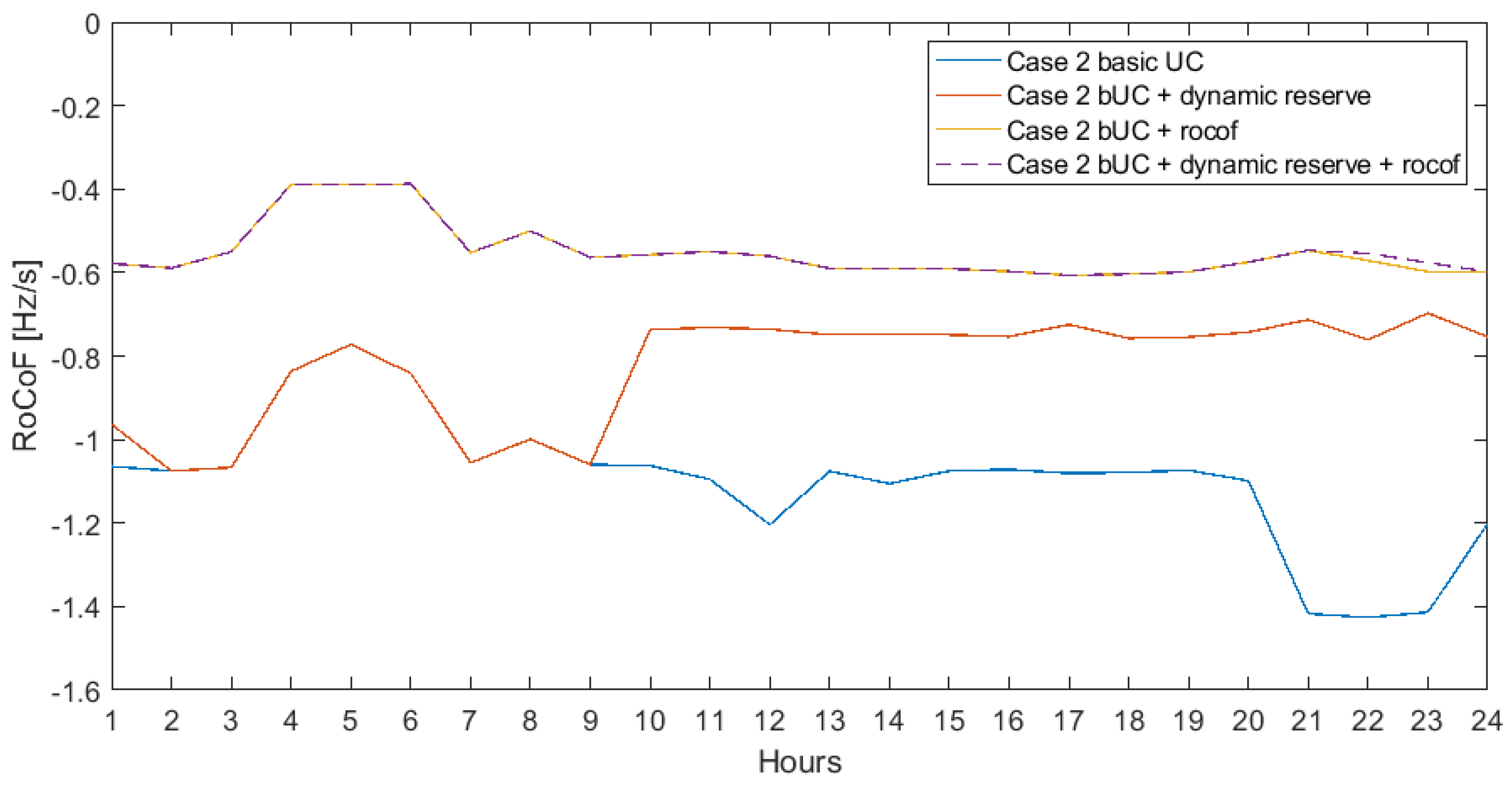
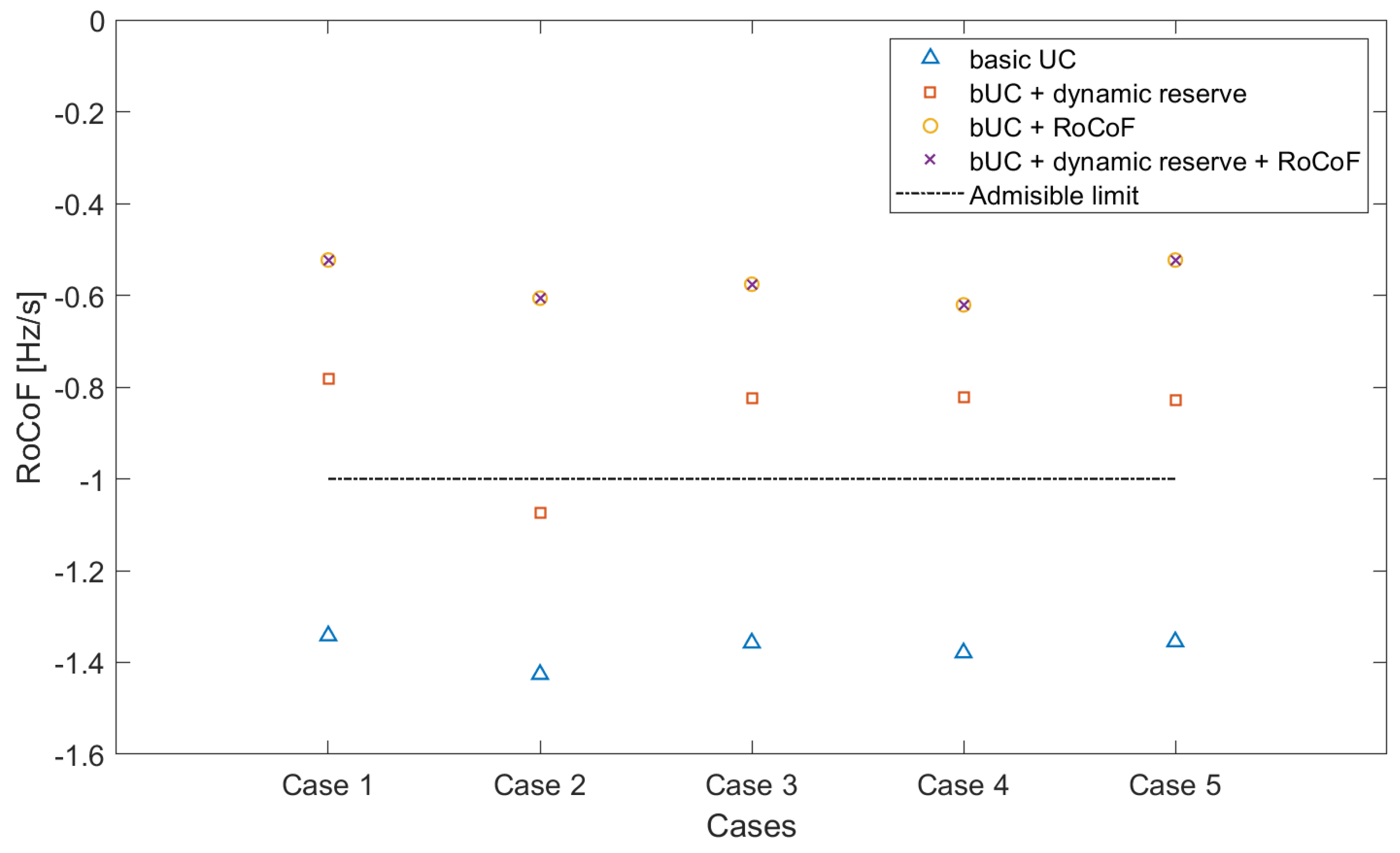
4.2. Frequency-Constrained Unit Commitment
5. Discussion and Conclusions
Author Contributions
Funding
Institutional Review Board Statement
Informed Consent Statement
Data Availability Statement
Acknowledgments
Conflicts of Interest
References
- Ministerio de Energía, Turismo y Agenda Digital, España, Resolución de 1 de febrero de 2018 de la Secretaría de Estado de Energía por la que se Aprueba el Procedimiento de Operación 12.2 “Instalaciones Conectadas a la Red de Transporte y Equipo Generador: Requisitos mínimos de Diseño, Equipamiento, Funcionamiento, Puesta en Servicio y Seguridad” de los Sistemas Eléctricos No Peninsulares. 2018. Available online: https://www.boe.es/boe/dias/2018/02/16/pdfs/BOE-A-2018-2198.pdf (accessed on 1 November 2019).
- Daly, P.; Flynn, D.; Cunniffe, N. Inertia considerations within unit commitment and economic dispatch for systems with high non-synchronous penetrations. In Proceedings of the 2015 IEEE Eindhoven PowerTech, Eindhoven, The Netherlands, 29 June–2 July 2015; pp. 1–6. [Google Scholar]
- Kundur, P. Power System Stability and Control; McGraw-Hill: New York, NY, USA, 1994. [Google Scholar]
- Lokay, H.E.; Burtnyk, V. Application of Underfrequency Relays for Automatic Load Shedding. IEEE Trans. Power Appar. Syst. 1968, PAS-87, 776–783. [Google Scholar] [CrossRef]
- Xie, L.; Carvalho, P.M.S.; Ferreira, L.A.F.M.; Liu, J.; Krogh, B.H.; Popli, N.; Ilić, M.D. Wind Integration in Power Systems: Operational Challenges and Possible Solutions. Proc. IEEE 2011, 99, 214–232. [Google Scholar] [CrossRef]
- Sigrist, L.; Lobato, E.; Echavarren, F.; Egido, I.; Rouco, L. Island Power Systems; CRC Press Taylor & Francis Group: Boca Raton, FL, USA, 2016. [Google Scholar]
- Jayawardena, A.V.; Meegahapola, L.G.; Perera, S.; Robinson, D.A. Dynamic characteristics of a hybrid microgrid with inverter and non- inverter interfaced renewable energy sources: A case study. In Proceedings of the 2012 IEEE International Conference on Power System Technology (POWERCON), Auckland, New Zealand, 23–26 October 2012; pp. 1–6. [Google Scholar]
- Restrepo, J.F.; Galiana, F.D. Unit commitment with primary frequency regulation constraints. IEEE Trans. Power Syst. 2005, 20, 1836–1842. [Google Scholar] [CrossRef]
- Chang, G.W.; Chuang, C.; Lu, T.; Wu, C. Frequency-regulating reserve constrained unit commitment for an isolated power system. IEEE Trans. Power Syst. 2013, 28, 578–586. [Google Scholar] [CrossRef]
- Kërçi, T.; Milano, F. A Framework to embed the Unit Commitment Problem into Time Domain Simulations. In Proceedings of the 2019 IEEE International Conference on Environment and Electrical Engineering and 2019 IEEE Industrial and Commercial Power Systems Europe (EEEIC/I CPS Europe), Genova, Italy, 10–14 June 2019; pp. 1–5. [Google Scholar]
- Wu, Z.; Gao, W.; Gao, T.; Yan, W.; Zhang, H.; Yan, S.; Wang, X. State-of-the-art review on frequency response of wind power plants in power systems. J. Mod. Power Syst. Clean Energy 2018, 6, 1–16. [Google Scholar] [CrossRef] [Green Version]
- Cardozo, C.; Capely, L.; Dessante, P. Frequency constrained unit commitment. Energy Syst. 2017, 8, 31–56. [Google Scholar] [CrossRef]
- Fei, T.; Trovato, V.; Strbac, G. Stochastic scheduling with inertia-dependent fast frequency response requirements. In Proceedings of the 2016 IEEE Power and Energy Society General Meeting (PESGM), Boston, MA, USA, 17–21 July 2016; 1, p. 1. [Google Scholar] [CrossRef]
- Cardozo Arteaga, C. Optimisation of Power System Security with High Share of Variable Renewables: Consideration of the Primary Reserve Deployment Dynamics on a Frequency Constrained Unit Commitment Model. Ph.D. Thesis, Université Paris-Saclay (ComUE), Paris, France, 2016. [Google Scholar]
- Doherty, R.; Lalor, G.; O’Malley, M. Frequency control in competitive electricity market dispatch. IEEE Trans. Power Syst. 2005, 20, 1588–1596. [Google Scholar] [CrossRef]
- Cardozo, C.; Capely, L.; van Ackooij, W. Cutting plane approaches for the frequency constrained economic dispatch problems. Electr. Power Syst. Res. 2018, 156, 54–63. [Google Scholar] [CrossRef]
- Rabbanifar, P.; Amjady, N. Frequency-constrained unit-commitment using analytical solutions for system frequency responses considering generator contingencies. IET Gener. Transm. Distrib. 2020, 14, 3548–3560. [Google Scholar] [CrossRef]
- Lemaréchal, C.; Renaud, A. A geometric study of duality gaps, with applications. Math. Program. 2001, 90, 399–427. [Google Scholar] [CrossRef]
- Van Ackooij, W. Large-scale unit commitment under uncertainty: An updated literature survey. Ann. Oper. Res. Univ. Pisa 2018, 271, 11–85. [Google Scholar] [CrossRef] [Green Version]
- Ummels, B.C.; Gibescu, M.; Pelgrum, E.; Kling, W.L.; Brand, A.J. Impacts of Wind Power on Thermal Generation Unit Commitment and Dispatch. IEEE Trans. Energy Convers. 2007, 22, 44–51. [Google Scholar] [CrossRef] [Green Version]
- Tuohy, A.; Denny, E.; Meibom, P.; Barth, R.; O’Malley, M. Operating the Irish power system with increased levels of wind power. In Proceedings of the 2008 IEEE Power and Energy Society General Meeting—Conversion and Delivery of Electrical Energy in the 21st Century, Pittsburgh, PA, USA, 20–24 July 2008; pp. 1–4. [Google Scholar]
- Zhang, Z.; Du, E.; Teng, F.; Zhang, N.; Kang, C. Modeling Frequency Dynamics in Unit Commitment With a High Share of Renewable Energy. IEEE Trans. Power Syst. 2020, 35, 4383–4395. [Google Scholar] [CrossRef]
- Melhorn, A.C.; Mingsong, L.; Carroll, P.; Flynn, D. Validating unit commitment models: A case for benchmark test systems. In Proceedings of the 2016 IEEE Power and Energy Society General Meeting (PESGM), Boston, MA, USA, 17–21 July 2016; pp. 1–5. [Google Scholar] [CrossRef] [Green Version]
- Aik, D.L.H. A general-order system frequency response model incorporating load shedding: Analytic modeling and applications. IEEE Trans. Power Syst. 2006, 21, 709–717. [Google Scholar] [CrossRef]
- Ela, E.; O’Malley, M. Studying the Variability and Uncertainty Impacts of Variable Generation at Multiple Timescales. IEEE Trans. Power Syst. 2012, 27, 1324–1333. [Google Scholar] [CrossRef] [Green Version]
- Ahmadi, H.; Martí, J.R.; Moshref, A. Piecewise linear approximation of generators cost functions using max-affine functions. In Proceedings of the 2013 IEEE Power Energy Society General Meeting, Vancouver, BC, Canada, 21–25 July 2013; pp. 1–5. [Google Scholar] [CrossRef]
- Ahmadi, H.; Ghasemi, H. Security-Constrained Unit Commitment With Linearized System Frequency Limit Constraints. IEEE Trans. Power Syst. 2014, 29, 1536–1545. [Google Scholar] [CrossRef]
- Riaz, S.; Verbič, G.; Chapman, A.C. Computationally Efficient Market Simulation Tool for Future Grid Scenario Analysis. IEEE Trans. Smart Grid 2019, 10, 1405–1416. [Google Scholar] [CrossRef] [Green Version]
- Ministerio para la Transición Ecológica y el Reto Demográfico, España, (EOLCAN) Ayudas a la Inversión en Instalaciones de Producción de Energía Eléctrica de Tecnología Eólica Situadas en Canarias. 2020. Available online: https://sede.idae.gob.es/lang/extras/tramites-servicios/2020/EOLCAN_2/Resolucion_IDAE_convocatoria_EOLCAN_2.pdf (accessed on 1 April 2021).
- Ministerio para la Transición Ecológica y el Reto Demográfico, España, (SOLCAN) Programa de Ayudas a la Inversión en Instalaciones de Producción de Energía Eléctrica de Tecnología Solar Fotovoltaica Situadas en Canarias Cofinanciadas con Fondos Comunitarios FEDER. 2020. Available online: https://sede.idae.gob.es/lang/extras/tramites-servicios/2020/SOLCAN/Resolucion_convocatoria_Solcan_de_24_de_junio_de_2020.pdf (accessed on 1 April 2021).
- Ministerio Para la Transición Ecológica y el Reto Demográfico, España, Investment Aid Programme for Electrical Energygeneration Installations with Wind Power Technology Located in Canarias, Co-Financed with Community Funds from the Erdf. 2021. Available online: https://www.pap.hacienda.gob.es/bdnstrans/GE/es/convocatoria/633341/document/254913 (accessed on 1 March 2021).
- Tseng, C.L. On Power System Generation unit Commitment Problems. Ph.D. Thesis, University of California, Berkeley, CA, USA, 1996. [Google Scholar]
- Paturet, M. Economic Valuation and Pricing of Inertia in Inverter-Dominated Power Systems. Master’s Thesis, Swiss Federal Institute of Technology (ETH), Zurich, Switzerland, 2019. Available online: https://arxiv.org/abs/2005.11029 (accessed on 1 March 2021).
- Badesa, L.; Teng, F.; Strbac, G. Pricing inertia and Frequency Response with diverse dynamics in a Mixed-Integer Second-Order Cone Programming formulation. Appl. Energy 2020, 260, 114334. [Google Scholar] [CrossRef] [Green Version]
- Richard, T.; Byerly, E.W.K. Stability of Large Electric Power Systems; IEEE Press: New York, USA, 1974. [Google Scholar]
- Estudios de Prospectiva del Sistema y Necesidades para su Operabilidad, Red Eléctrica de España. 2020. Available online: https://www.ree.es/sites/default/files/01_ACTIVIDADES/Documentos/Prospectiva_y_Operabilidad_Reunion_GSP29Sep20.pdf (accessed on 1 May 2021).
- Rodríguez-Bobada, F.; Izquierdo, C.; Soto, J.; Cuevas, R.; Santos, P.; Corujo, R. Simplified Frequency Stability Tool for Isolated Systems: ADin. In Proceedings of the 3rd International Hybrid Power Systems Workshop, Tenerife, Spain, 8–9 May 2018. [Google Scholar]
- MATLAB. Version R2020b; The MathWorks Inc.: Natick, MA, USA, 2020. [Google Scholar]
- Ministerio de Industria, Energía Y Turismo, España, Real Decreto 738/2015 de 31 de Julio por el que se Regula la Actividad de Producción de Energía Eléctrica y el Procedimiento de Despacho en los Sistemas Eléctricos de los Territorios no Peninsulares. 2015. Available online: https://www.boe.es/boe/dias/2015/08/01/pdfs/BOE-A-2015-8646.pdf (accessed on 1 May 2021).
- REE Web Repository of Historical Hourly Generation Data. 2021. Available online: https://demanda.ree.es/visiona/canarias/gcanaria/ (accessed on 1 May 2021).
- El Sistema Eléctrico Español,2019, Departamento de Acceso a la Información del Sistema Eléctrico de REE, Red Eléctrica de España. 2020. Available online: https://www.ree.es/sites/default/files/11_PUBLICACIONES/Documentos/InformesSistemaElectrico/2019/inf_sis_elec_ree_2019.pdf (accessed on 1 May 2021).
- ENTSO-E Network Code for Requirements for Grid Connection Applicable to all Generators, European Network of Transmission System Operators (ENTSO-E). 2013. Available online: https://eepublicdownloads.entsoe.eu/clean-documents/pre2015/resources/RfG/130308_Final_Version_NC_RfG.pdf (accessed on 1 May 2021).
- Criterios Generales de Protección de los Sistemas Eléctricos Insulares y eXtrapeninsulares, Red Eléctrica de España. 2005. Available online: https://www.ree.es/sites/default/files/downloadable/criterios_proteccion_sistema_2005_v2.pdf (accessed on 1 May 2021).


| Adding Indirect Constraints | Post-Contingency Frequency Behavior Model | Directly Accounting for Frequency-Related Constraints in UC Models | |||
|---|---|---|---|---|---|
| Authors | Disadvantage | Authors | Disadvantage | Authors | Disadvantage |
| Restrepo (2005) [8] | More demanding computionally scheduling | Aik (2006) [24] | No guarantee of the dynamic stability of low-inertia systems | Teng (2016) [13] | Dynamics of the system are oversimplified |
| Ela (2012) [25] | Dynamics of the system are oversimplified and linearized | Ahmadi (2013) [26] | No guarantee of the dynamic stability of low-inertia systems | Cardozo (2018) [16] | Assumptions theoretically hard to verify |
| Ahmadi (2014) [27] | Cannot ensure satisfaction of the original constraint | Kerci (2019) [10] | No guarantee of the dynamic stability of low-inertia ystems | Rabbanifar (2020) [17] | Theoretically hard to verify |
| Riaz (2019) [28] | Dynamics of the system are oversimplified and linearized | - | - | - | - |
| Register Number | Power Plant Name | Max Power MW | Min Power MW | Discharge Date |
|---|---|---|---|---|
| RO2-0089 | BARRANCO DE TIRAJANA 1. GAS 1 | 32.34 | 6.79 | 01/07/1992 |
| RO2-0090 | BARRANCO DE TIRAJANA 2, GAS 2 | 32.34 | 6.79 | 11/05/1995 |
| RO1-1049 | BARRANCO DE TIRAJANA 3, VAPOR 1 | 74.24 | 27.84 | 01/01/1996 |
| RO1-1050 | BARRANCO DE TIRAJANA 4, VAPOR 2 | 74.24 | 27.84 | 05/06/1996 |
| RO1-1051 | 68.7 | 9.70 | 19/07/2003 | |
| RO1-1052 | BARRANCO DE TIRAJANA, CC1 | 103.05 | 37.80 | 21/08/2003 |
| RO1-2000 | 206,1 | 75.50 | 22/11/2004 | |
| RO2-0188 | 75.0 | 9.70 | 01/08/2006 | |
| RO2-0189 | BARRANCO DE TIRAJANA. CC2 | 113.5 | 37.80 | 27/11/2006 |
| RO2-0190 | 227.0 | 75.50 | 18/06/2008 | |
| RO2-0087 | JINAMAR 10. GAS 2 | 32.34 | 6.79 | 26/01/1989 |
| RO2-0088 | JINAMAR 11, GAS 3 | 32.34 | 6.79 | 01/05/1989 |
| RO2-0084 | JINAMAR 12, DIESEL 4 | 20.51 | 14.09 | 07/06/1990 |
| RO2-0085 | JINAMAR 13, DIESEL 5 | 20.51 | 14.09 | 08/08/1990 |
| RO2-0081 | JINAMAR 2, DIESEL 1 | 8.51 | 4.58 | 01/02/1973 |
| RO2-0082 | JINAMAR 3, DIESEL 2 | 8.51 | 4.58 | 27/08/1973 |
| RO2-0083 | JINAMAR 4, DIESEL 3 | 8.51 | 4.58 | 01/02/1974 |
| RO2-0086 | JINAMAR 7, GAS 1 | 17.64 | 6.79 | 21/04/1981 |
| RO1-1047 | JINAMAR 8, VAPOR 4 | 55.56 | 17.7 | 01/08/1982 |
| RO1-1048 | JINAMAR 9, VAPOR 5 | 55.56 | 17.7 | 05/12/1984 |
| Case | 1 | 2 | 3 | 4 | 5 |
|---|---|---|---|---|---|
| Hour | |||||
| 1 | 325.80 | 329.33 | 335.27 | 334.13 | 312.05 |
| 2 | 293.33 | 302.50 | 311.37 | 312.03 | 290.53 |
| 3 | 274.63 | 283.83 | 237.63 | 300.83 | 275.50 |
| 4 | 267.90 | 271.83 | 277.53 | 292.08 | 265.72 |
| 5 | 267.33 | 267.33 | 275.70 | 290.30 | 262.18 |
| 6 | 276.87 | 270.00 | 278.67 | 289.65 | 263.52 |
| 7 | 321.23 | 275.17 | 287.05 | 302.08 | 273.47 |
| 8 | 385.32 | 268.83 | 291.33 | 304.95 | 271.42 |
| 9 | 417.63 | 295.22 | 328.70 | 342.82 | 298.85 |
| 10 | 285.50 | 329.40 | 366.63 | 380.70 | 337.18 |
| 11 | 378.08 | 361.37 | 392.20 | 402.72 | 361.50 |
| 12 | 432.93 | 376.40 | 402.40 | 407.45 | 376.23 |
| 13 | 446.63 | 378.08 | 414.23 | 412.28 | 385.38 |
| 14 | 464.97 | 389.30 | 426.08 | 421.27 | 399.55 |
| 15 | 463.43 | 384.53 | 412.50 | 415.00 | 392.05 |
| 16 | 448.93 | 358.97 | 378.92 | 387.93 | 362.58 |
| 17 | 435.83 | 337.63 | 360.55 | 367.62 | 348.45 |
| 18 | 436.47 | 339.93 | 367.82 | 374.73 | 352.70 |
| 19 | 481.13 | 351.68 | 397.67 | 406.20 | 386.88 |
| 20 | 508.68 | 366.65 | 439.53 | 438.83 | 416.37 |
| 21 | 509.23 | 393.70 | 445.08 | 440.67 | 421.43 |
| 22 | 492.87 | 431.00 | 420.38 | 421.67 | 398.58 |
| 23 | 435.08 | 402.50 | 372.43 | 379.83 | 360.23 |
| 24 | 382.90 | 352.50 | 332.50 | 339.88 | 322.47 |
| Renewable Penetration (%) | 1.5% | 29.3% | 10.2% | 10.7% | 6.5% |
| Case Number | Constraints Used | |||
|---|---|---|---|---|
| Case 1 | bUC | dynamic reserve | RoCoF | dynamic reserve + RoCoF |
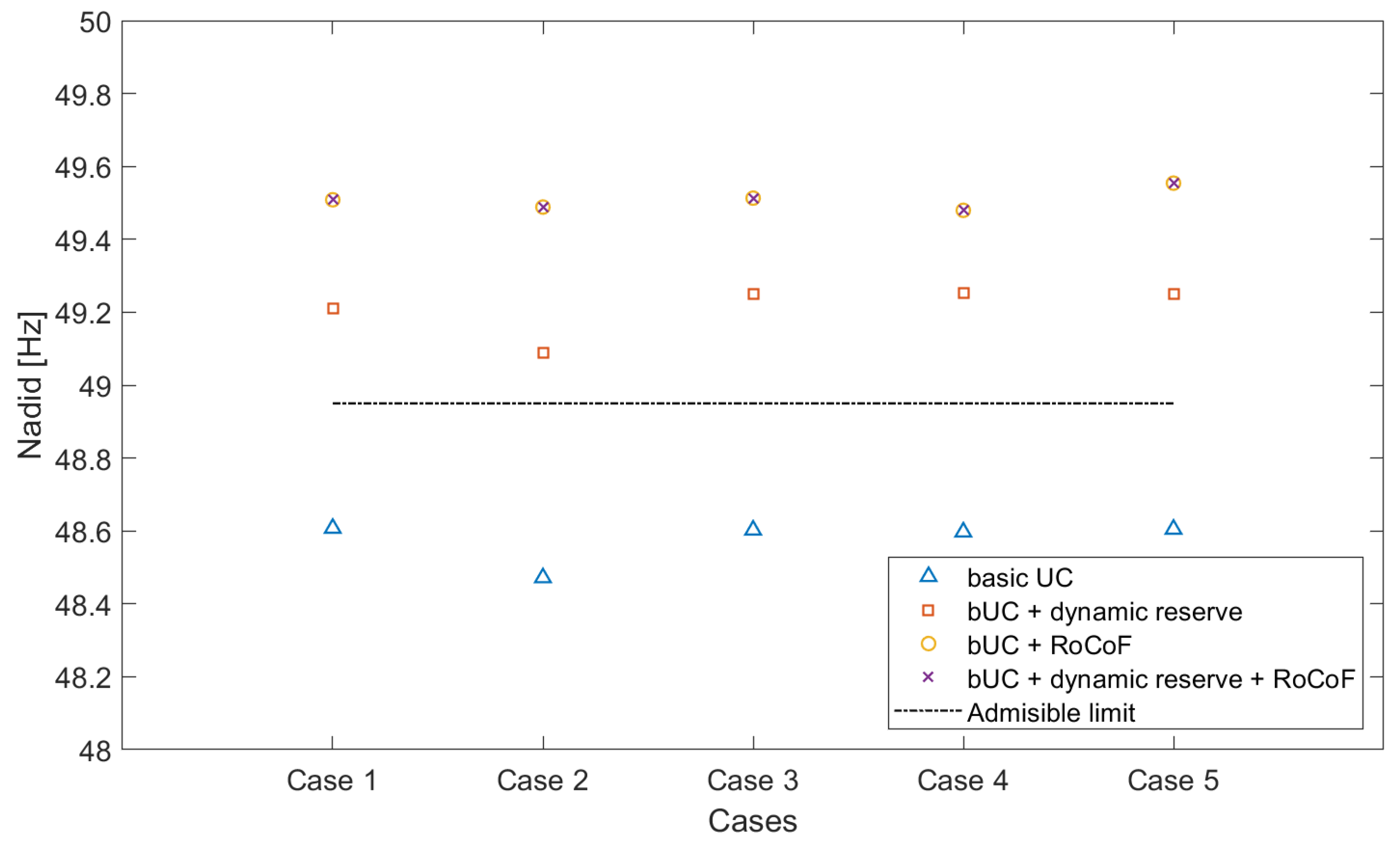
| Mín RoCoF (Hz/s) | −1.34 | −0.78 | −0.52 | −0.52 |
| Mín Nadir (Hz) | 48.61 | 49.21 | 49.51 | 49.51 |
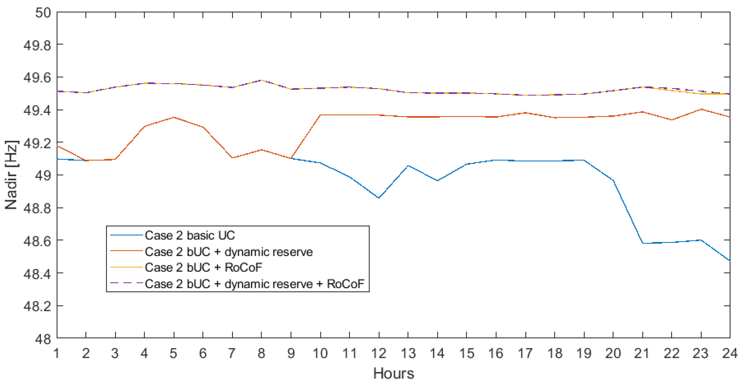
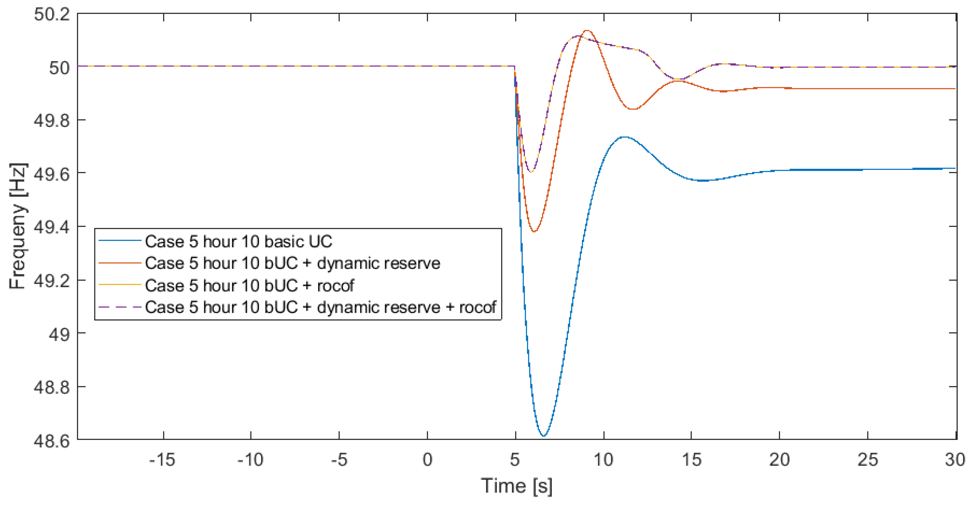
| Case 2 | bUC | dynamic reserve | RoCoF | dynamic reserve + RoCoF |
| Mín RoCoF (Hz/s) | −1.43 | −1.08 | −0.61 | −0.61 |
| Mín Nadir (Hz) | 48.47 | 49.09 | 49.49 | 49.49 |
| Case 3 | bUC | dynamic reserve | RoCoF | dynamic reserve + RoCoF |
| Mín RoCoF (Hz/s) | −1.36 | −0.82 | −0.58 | −0.58 |
| Mín Nadir (Hz) | 48.60 | 49.25 | 49.51 | 49.51 |
| Case 4 | bUC | dynamic reserve | RoCoF | dynamic reserve + RoCoF |
| Mín RoCoF (Hz/s) | −1.38 | −0.82 | −0.62 | −0.62 |
| Mín Nadir (Hz) | 48.60 | 49.25 | 49.48 | 49.48 |
| Case 5 | bUC | dynamic reserve | RoCoF | dynamic reserve + RoCoF |
| Mín RoCoF (Hz/s) | −1.35 | −0.83 | −0.52 | −0.52 |
| Mín Nadir (Hz) | 48.60 | 49.25 | 49.55 | 49.55 |
| Case Number and Cost Breakdown | Constraints Used | |||
|---|---|---|---|---|
| Case 1 | bUC | dynamic reserve | RoCoF | dynamic reserve + RoCoF |
| Start-Up Cost (EUR) | 82,739 | 91,506 | 91,506 | 91,506 |
| Regulation Cost (EUR) | 7926 | 8078 | 8322 | 8322 |
| Operational Cost (EUR) | 792,625 | 807,780 | 832,158 | 832,158 |
| O&M Cost (EUR) | 212 | 212 | 207 | 207 |
| Total Operation Cost (EUR) | 883,502 | 907,576 | 932,192 | 932,192 |
| Case 2 | bUC | dynamic reserve | RoCoF | dynamic reserve + RoCoF |
| Start-Up Cost (EUR) | 0 | 33,397 | 24,629 | 29,013 |
| Regulation Cost (EUR) | 4461 | 4539 | 4744 | 4747 |
| Operational Cost (EUR) | 446,056 | 453,857 | 474,372 | 474,627 |
| O&M Cost (EUR) | 136 | 134 | 133 | 134 |
| Total Operation Cost (EUR) | 450,652 | 491,926 | 503,879 | 508,519 |
| Case 3 | bUC | dynamic reserve | RoCoF | dynamic reserve + RoCoF |
| Start-Up Cost (EUR) | 24,629 | 42,164 | 78,355 | 78,355 |
| Regulation Cost (EUR) | 6372 | 6594 | 6410 | 6410 |
| Operational Cost (EUR) | 637,162 | 659,372 | 641,047 | 641,047 |
| O&M Cost (EUR) | 173 | 172 | 177 | 177 |
| Total Operation Cost (EUR) | 668,336 | 708,302 | 725,990 | 725,990 |
| Case 4 | bUC | dynamic reserve | RoCoF | dynamic reserve + RoCoF |
| Start-Up Cost (EUR) | 24,629 | 42,164 | 73,972 | 73,972 |
| Regulation Cost (EUR) | 6432 | 6682 | 6519 | 6519 |
| Operational Cost (EUR) | 643,193 | 668,192 | 651,928 | 651,928 |
| O&M Cost (EUR) | 178 | 176 | 180 | 180 |
| Total Operation Cost (EUR) | 674,432 | 717,214 | 732,599 | 732,599 |
| Case 5 | bUC | dynamic reserve | RoCoF | dynamic reserve + RoCoF |
| Start-Up Cost (EUR) | 24,629 | 37,780 | 78,355 | 29,013 |
| Regulation Cost (EUR) | 6209 | 6476 | 6340 | 4746 |
| Operational Cost (EUR) | 620,934 | 647,570 | 634,025 | 474,627 |
| O&M Cost (EUR) | 174 | 171 | 176 | 134 |
| Total Operation Cost (EUR) | 651,946 | 691,997 | 718,897 | 718,897 |
| Operational Cost Increase in Percentage | |||||
|---|---|---|---|---|---|
| Constraint | Case 1 | Case 2 | Case 3 | Case 4 | Case 5 |
| Dynamic reserve | 2.72% | 9.16% | 5.98% | 6.34% | 6.14% |
| RoCoF | 5.51% | 11.81% | 8.63% | 8.62% | 10.27% |
| Dynamic reserve + RoCoF | 5.51% | 12.84% | 8.63% | 8.62% | 10.27% |
Publisher’s Note: MDPI stays neutral with regard to jurisdictional claims in published maps and institutional affiliations. |
© 2021 by the authors. Licensee MDPI, Basel, Switzerland. This article is an open access article distributed under the terms and conditions of the Creative Commons Attribution (CC BY) license (https://creativecommons.org/licenses/by/4.0/).
Share and Cite
Rebollal, D.; Chinchilla, M.; Santos-Martín, D.; Guerrero, J.M. Endogenous Approach of a Frequency-Constrained Unit Commitment in Islanded Microgrid Systems. Energies 2021, 14, 6290. https://doi.org/10.3390/en14196290
Rebollal D, Chinchilla M, Santos-Martín D, Guerrero JM. Endogenous Approach of a Frequency-Constrained Unit Commitment in Islanded Microgrid Systems. Energies. 2021; 14(19):6290. https://doi.org/10.3390/en14196290
Chicago/Turabian StyleRebollal, David, Mónica Chinchilla, David Santos-Martín, and Josep M. Guerrero. 2021. "Endogenous Approach of a Frequency-Constrained Unit Commitment in Islanded Microgrid Systems" Energies 14, no. 19: 6290. https://doi.org/10.3390/en14196290
APA StyleRebollal, D., Chinchilla, M., Santos-Martín, D., & Guerrero, J. M. (2021). Endogenous Approach of a Frequency-Constrained Unit Commitment in Islanded Microgrid Systems. Energies, 14(19), 6290. https://doi.org/10.3390/en14196290