Article

Optimized Fuzzy Skyhook Control for Semi-Active Vehicle Suspension with New Inverse Model of Magnetorheological Fluid Damper

1
State Key Laboratory of Engines, Tianjin University, Tianjin 300072, China
2
School of Engineering, RMIT University, Melbourne, VIC 3000, Australia
3
Shantui Construction Machinery CO., LTD, Jining 272000, China
*
Author to whom correspondence should be addressed.
Energies 2021, 14(6), 1674; https://doi.org/10.3390/en14061674
Submission received: 10 February 2021 / Revised: 12 March 2021 / Accepted: 12 March 2021 / Published: 17 March 2021

Abstract

:
To improve the performance of vehicle suspension, this paper proposes a semi-active vehicle suspension with a magnetorheological fluid (MRF) damper. We designed an optimized fuzzy skyhook controller with grey wolf optimizer (GWO) algorithm base on a new neuro-inverse model of the MRF damper. Because the inverse model of the MRF damper is difficult to establish directly, the Elman neural network was applied. The novelty of this study is the application of the new inverse model for semi-active vibration control and optimization of the semi-active suspension control method. The calculation results showed that the new inverse model can accurately calculate the required control current. The fuzzy skyhook control method optimized by the grey wolf optimizer (GWO) algorithm was established based on the inverse model to control the suspension vibration. The simulation results showed that the optimized fuzzy skyhook control method can simultaneously reduce the amplitude of vertical acceleration, suspension deflection, and tire dynamic load.

Graphical Abstract

1. Introduction

Magnetorheological fluid (MRF) is an intelligent material that can transform between a Newtonian fluid state and a semi-solid state according to the strength of the magnetic field. The ferromagnetic particles of MRF are randomly distributed without an external magnetic field, so MRF performs as a Newtonian fluid and can flow under only small shear. Furthermore, the ferromagnetic particles in MRF rearrange along the direction of the magnetic field. The higher the strength of the magnetic field, the denser the arrangement of the ferromagnetic particles. Finally, MRF exhibits semi-solid properties, and much greater shear force is required to make it flow. When the applied magnetic field disappears suddenly, the MRF material can return to its original state in milliseconds [1,2].
Due to the fact of its variable and controllable properties, an MRF damper is considered to have great potential in vibration mitigation. The damping force of an MRF damper can vary with the applied current or voltage due to the change in the magnetic field strength [3,4].
For vehicle vibration reduction, to improve the performance of vehicle suspension, the main schemes include active and semi-active suspensions. Although active suspension better reduces vibrations, it also has some disadvantages, such as complex structure, high cost, and high energy consumption, which limit its application in mass production vehicles [5]. With the help of a control algorithm, semi-active suspension represented by an MRF damper can achieve the desirable effect of active control without high-cost hardware.
When the MRF damper is applied to vehicle suspension, a precise mechanical model of the damping force is essential for vibration control. The mechanical model of the MRF damper can reflect the relationships between the damping force and the relative displacement, the relative velocity, and the current. At present, two kinds of models—the physical model and the phenomenological model—are used to describe the working characteristics of the MRF damper [6]. The latter is usually applied to vibration control, for which parameters are identified from the relationships between the damping force produced by the MRF damper and the piston velocity, current, and the piston displacement. Commonly used phenomenological models include the Bouc-Wen model [7,8], the Bingham model [9], the Dahl model [10], and the polynomial model [11]. Using these models, the corresponding relationships between the damping force and relative displacement, relative velocity, and current can be reflected accurately. Among these magnetorheological models, the Bouc-Wen model is widely used because it can accurately reflect the displacement and velocity characteristics of the MRF damper and has high fitting accuracy.
The Bouc-Wen and other models can accurately reflect the relationships between the damping force and relative displacement, velocity, and current. However, in semi-active control, the control current should be inversely calculated from the damping force which is calculated by the control algorithm. Thus, an inverse model of the MRF damper should be built to calculate the control current from the expected damping force. However, due to the obvious nonlinear characteristics of the relationship between the output damping force of the MRF damper and its control current, piston displacement, and velocity, it is difficult to obtain the inverse model of the MRF damper through phenomenological models from which the control current can be directly calculated from the expected damping force. To achieve better vibration reduction, the inverse model of the MRF damper should be able to accurately provide the control current, and the structure should be simple and easy to use [12]. The current research results show that technology based on artificial intelligence (AI) can build an MRF damper inverse model using machine learning methods [13]. Nguyen [14] developed a new neural fuzzy system algorithm to identify the dynamic characteristics of MR and electrorheological (ER) dampers and proposed an algorithm, which was validated. The back propagation (BP) neural network was mapped from the desired damping force to the control voltage by inputting variables [15]. Although the prediction accuracy of the BP neural network is acceptable, it has some shortcomings. The BP neural network does not have a feedback structure and cannot obtain a good prediction effect when dealing with unstable and irregular signals. To solve this problem, the Elman neutral network was used to build the inverse model of the MRF damper. The Elman neural network is a multi-layer feedforward neural network that is based on the BP neural network and introduces a negative feedback system. Compared with the BP neural network, the Elman neural network has better stability and is better at classifying the original data [16].
In the field of vehicle ride comfort and vibration control, we have conducted research work. We established a vibration model of the human body in the vertical direction to lay the foundation for the active control of vehicle seat vibration [17]. We also applied the fuzzy PID (proportional–integral–derivative) control method to the vibration reduction of the vehicle seat and carried out simulation analysis [18]. The results show that the active control method can clearly improve the vehicle ride comfort.
However, these control studies used active control methods and are not suitable for direct application to the semi-active control of the MRF damper. Therefore, we studied the semi-active control method. Many studies have been conducted on the control algorithm for MRF suspension. Weber [19] developed a robust force tracking control method to control the MRF damper, and the proposed algorithm was validated. Weber [20] used the non-linear adaptive damping control method to realize the real-time semi-active control of the MRF damper. Yu [21] designed a fuzzy logical control algorithm for achieving vibration isolation of the MR damper. From the perspective of the control force output, the control force is the damping force of the MRF damper, so the direction of the control force can only be the same as the direction of the damping force produced by the MRF damper. The output law of the fuzzy skyhook control method coincides with the characteristics of the damper. Therefore, the fuzzy skyhook control method was selected to control the MRF suspension system.
In the fuzzy control method, the two control inputs must be multiplied by quantitative factors, Ka and Kv, then calculated using fuzzy rules. The calculation result of the fuzzy controller must be multiplied by a scale factor Ku and then output as the control result.
To perform well, fuzzy controllers must have a reasonable choice of quantitative factors Ka, Kv, and scale factor Ku. These parameters have a certain regulating effect on the control performance. Increasing the quantization factor, Ka, can speed up the rising rate of the system, but can also lead to an increase in overshoot. Increasing the quantization factor, Kv, can improve the stability of the system. However, if Kv is too large, the system rise rate process is too slow. Increasing the scale factor Ku will make the system respond faster, but too large a value of Ku can cause the system to overshoot and undergo oscillation dispersion. However, these three parameters are generally selected based on experience, so it is difficult to obtain the best control effect. The grey wolf algorithm is a new intelligent optimization algorithm with the characteristics of a simple principle, few adjustment parameters, and low computational requirement, and it has been widely used in the field of parameter optimization [22]. Therefore, the grey wolf optimizer algorithm was used in this study to optimize the parameters, or quantification factors Ka and Kv, and the scale factor Ku in the fuzzy control to achieve the best control effect.
The research route of this paper can be summarized as follows: Because the semi-active control algorithm is used for the MRF damper, the MRF damper control force output is determined by the input current. Therefore, it is necessary to establish a reliable method to control the current through the output damping force of the MRF damper. Because of the complexity of the dynamic model of the MRF damper, the neural network method was used. At present, the BP neural network is usually used to establish the inverse model, and the accuracy of the model needs to be improved. Therefore, in this study, an Elman neural network was used to establish the inverse model of the MRF damper, which can obtain a control current according to the control force that is calculated by the control algorithm.
Regarding semi-active control, the fuzzy skyhook control method is a suitable control method for the MRF damper. However, the selection of key parameters Ka, Kv, and Ku in fuzzy control is not accurate and mainly depends on experience. Therefore, to address this problem, this study optimized fuzzy control to obtain a better suspension damping effect. The schematic of the research workflow is shown in Figure 1.
The main work of this paper is shown as follows: the mechanical properties of the MRF damper were tested, and the dynamic model of the MRF damper was established based on the Bouc-Wen model. To obtain accurate results of the control current, the inverse model of the MRF damper was modeled and trained using the Elman neural network. Finally, the neural network inverse model was applied to the semi-active control of the quarter vehicle suspension system. The fuzzy skyhook method was used to control the suspension vibration. Aiming to overcome the shortcomings of the fuzzy control approach, the GWO algorithm was used to optimize the quantization factors and the scale factor in the fuzzy controller to obtain a satisfactory control effect. The analysis results indicate that the dynamic performance of the vehicle suspension improved, and the inverse model of the MRF damper proposed in this paper was validated.

2. Dynamic Model of the MRF Damper

2.1. Mechanical Test of the MRF Damper

The structure of the MRF damper is shown in Figure 2. It is composed of a cylinder block, piston, floating piston, magnetorheological fluid, coil, sealing ring, gas chamber, and coil lead wire. There is an orifice on the piston and a coil wound around the piston to generate a strong magnetic field.
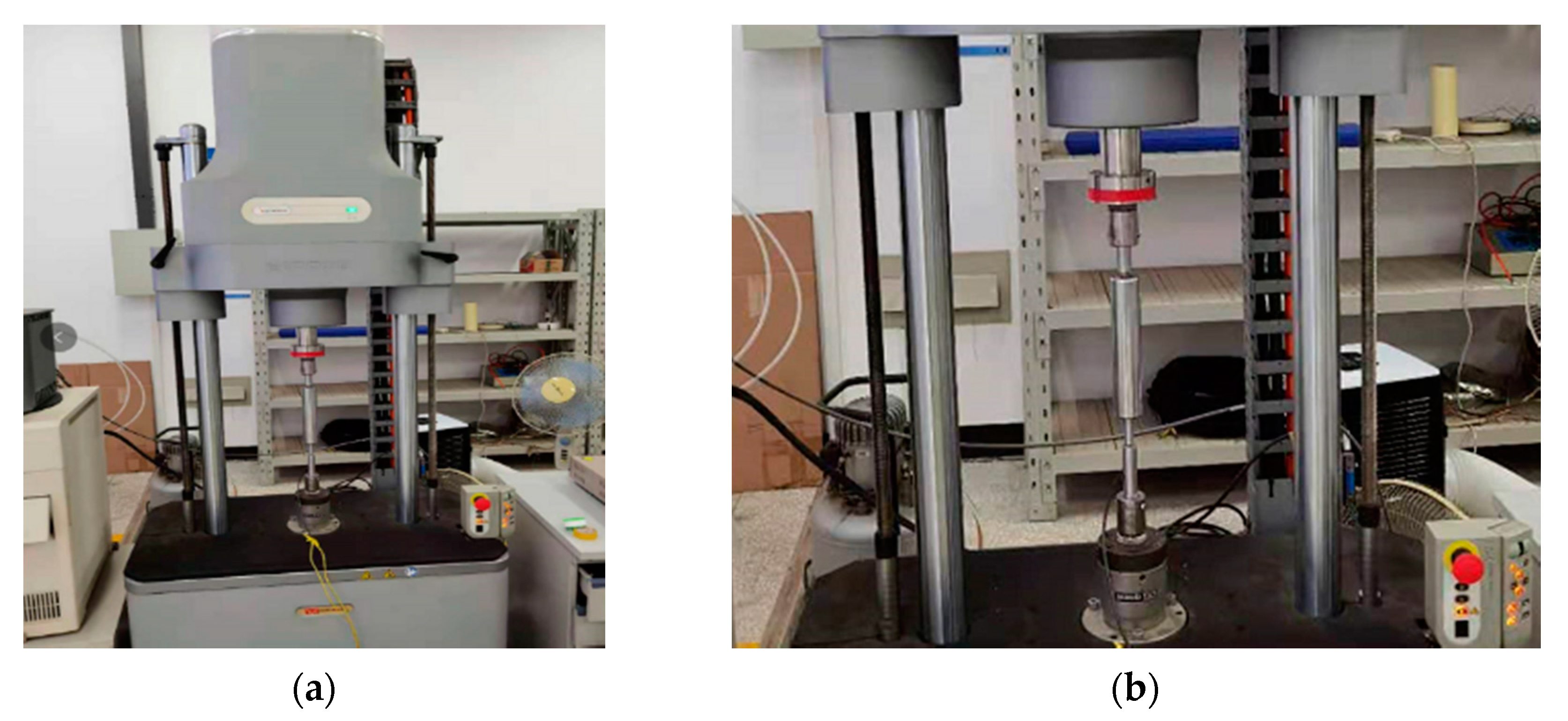
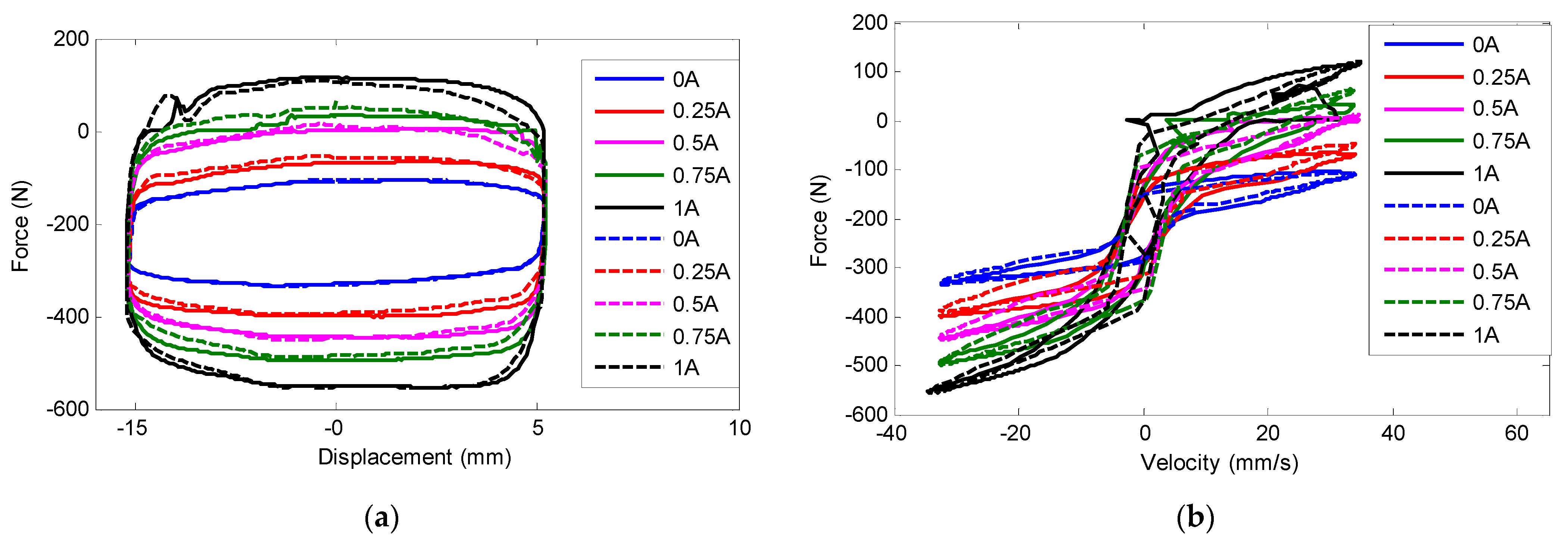
To obtain the damping characteristics of the MRF damper, the magnetorheological fluid damper was installed on the Instron E10000 electronic dynamic testing machine (manufactured by Instron company in Boston, US) as shown in Figure 3. In the test, the excitation frequency and amplitude could set to make the MRF damper piston move up and down under the action of the dynamic testing machine, and the input current of the MRF damper was controlled by a DC power supply. In this experiment, the set current was 0, 0.25, 0.5, 0.75, and 1 A; the displacement input excitation was 5 and 10 mm; the frequency was 0.5, 1, and 2 Hz, for a total of 30 working conditions. Due to the large number of working conditions, we used the 5 mm, 1 Hz working condition as an example for analysis as shown in Figure 4.
Figure 4 shows that the shape of the damping force and displacement curve of the MRF damper was rectangular and full, which indicates that the damper has good vibration attenuation ability. Under the same amplitude and frequency excitation, the higher the input current, the greater the output damping force of the MRF damper. The force–velocity curve of the MRF damper was approximately a symmetric hyperbola with obvious hysteresis characteristics. When the relative velocity of the MRF damper piston was small, the MRF damper presented the hysteresis phenomenon, and the area of the hysteresis loop increased with the increase in the input current; when the relative velocity of the damper piston was large, the curve shows shear phenomenon, revealing that the MRF damper has strong nonlinear dynamic characteristics.

2.2. Bouc-Wen Model

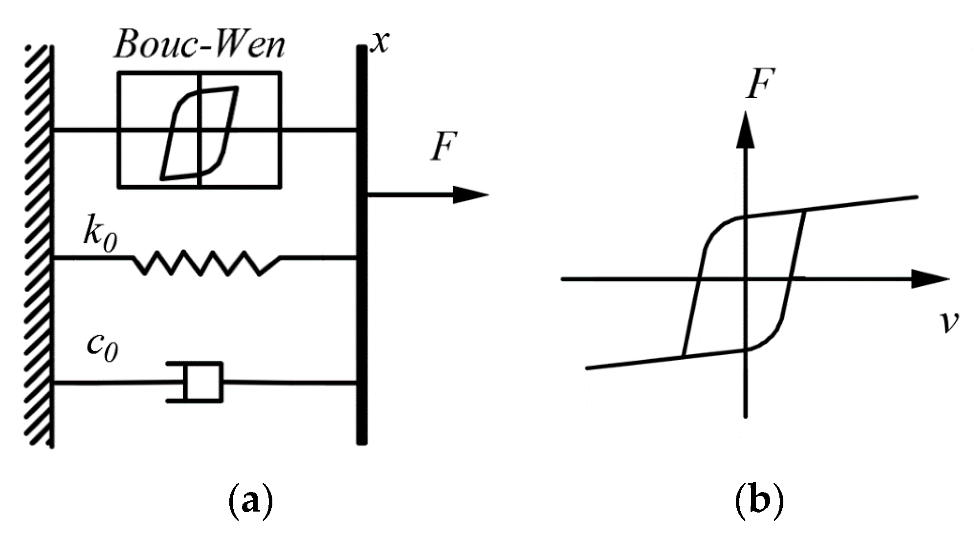
To fully utilize the semi-active characteristic of the MRF damper, we need to build an accurate dynamic model to achieve the real-time performance of semi-active control. Among various models, the Bouc-Wen model is the most commonly used [6,7], and describes the hyperbolic hysteresis characteristics of the MRF damper. It is made of a linear spring, a linear damper, and a hysteretic element in parallel. As shown in Figure 5, the hysteresis curve function was added to describe the hysteretic characteristics of the MRF damper. The damping force of the MRF damper is shown as follows:
{ F = c 0 x ˙ + k 0 ( x x 0 ) + α z z ˙ = γ | x ˙ | z | z | n 1 β x ˙ | z | n + A x ˙
where F is the damping force, c0 is the viscosity coefficient, k0 is the stiffness coefficient, α is the proportion adjustment parameter of the hysteretic force in the damping force, x0 is the relative equilibrium displacement, z is the hysteretic variable, x and x ˙ are the relative displacement and relative velocity at both ends of the damping, respectively, n is the smoothing coefficient, and γ, β, and A are parameters used to adjust the smoothness of the model and the linear characteristics from the yield area to the post-yield area of the curve.
Because this model can better describe the relationship between the output damping force and the piston speed, it can also better reflect the hysteresis characteristics of the magnetorheological fluid damper, so we selected this method to fit the MRF damper dynamic model.

2.3. The Dynamic Model of MRF Damper

The eight unknown parameters of the Bouc-Wen model were difficult to identify due to the relationship between the Bouc-Wen model and the current. Using the Simulink Design Optimization toolbox [23], the measured displacement and velocity were taken as inputs to calculate the damping force using the landmark programming of interconnection by adjusting the vector of unknown parameters. Then, the calculated result was compared with the test results.
The parameter identification steps were as follows:
(1)
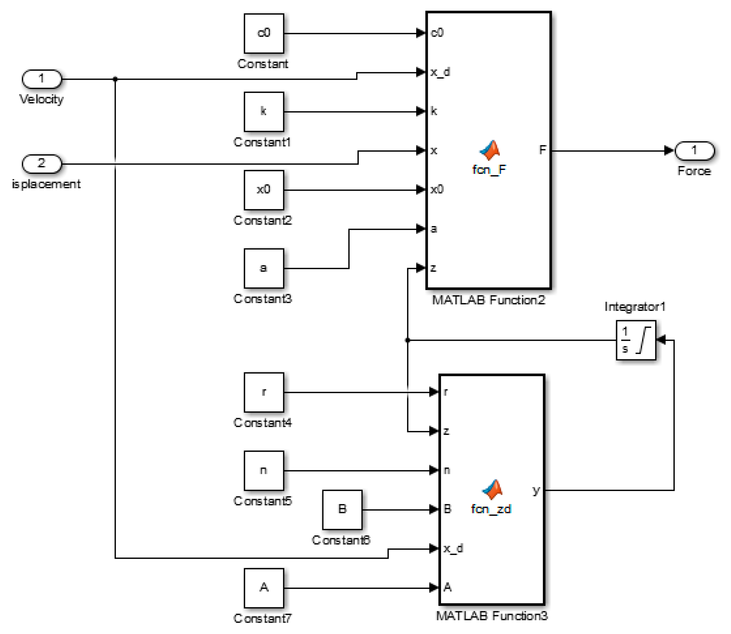
Build the Bouc-Wen model in Simulink. The model is shown in Figure 6.
(2)
Import the test data. The test data of sinusoidal excitation with 5 mm, 1 Hz shown in Figure 3 under different current conditions were imported into the Simulink model. The input values of the model were displacement and velocity, and the output value was damping force.
(3)
Select the parameters to identify. The Bouc-Wen model has eight unknown parameters; first, set an initial value first, and then start to identify. The initial values are listed in Table 1.
(4)
In the process of parameter identification, the parameters have different effects on the Bouc-Wen model. It was found that γ and β only affect the shape of the hysteresis loop but not the magnitude of the damping force, and n only affects the smoothness of the transition curve from the elastic zone to the plastic zone [8]. From Figure 4, it can be seen that the magnitude of the current has a great influence on the damping force amplitude. Through the preliminary identification of the model parameters, we found that the values of parameters A, α, and c0 vary greatly with the current, so it was assumed that a relationship can be developed between A, α, c0 and the magnitude of current. The other parameters were fixed as constants. The parameters identified are listed in Table 2.
After the parameter recognition of the Bouc-Wen model was completed, the output damping force can be calculated by inputting the displacement, velocity, and current of the MRF damper, and then the displacement–force curve and velocity–force curve can be simulated.
To verify the model identification results, the simulation results were compared with the test data under different currents as shown in Figure 7. In the Figure 7, the experimental data are shown as solid lines and the simulation results are dotted lines. In the Figure 7, we can see that the calculated displacement–force curve and the velocity–force curve by the Bouc-Wen model identified in the article are good and consistent with the experimental result.
The parameters of the Bouc-Wen model were obtained under a specific case of 1 Hz sinusoidal excitation of 5 mm amplitude, so the generality of the model (i.e., the dynamic response under other excitations) was also tested. The working condition of 0.5 Hz, 10 mm with 0.25 A current was selected for analysis. The sinusoidal excitation signal of this working condition was input into the Bouc-Wen model identified in Table 2 to calculate the damping force. The displacement damping force current and velocity damping force current were determined, then compared with the test results as shown in Figure 8.
From Figure 8, we can see that the proposed model can accurately reflect the dynamic response of the MRF damper under sinusoidal excitation in other cases, it has good universality.

3. The Inverse Dynamic Model of MRF Damper

In the semi-active control, the control force can be calculated by the control algorithm, which needs to be output by the MRF damper. At this time, it is necessary to regulate the current of the MRF damper to change the output damping force. Therefore, it is necessary to build an inverse dynamic model of the MRF damper to calculate the control current from the expected damping force.
Because the relationship between the output force and the control current of the MRF damper is complex, the mathematical expression of the relationship between them cannot be calculated directly. Thus, the neural network method was used to establish the relationship between them to predict the required control current according to the expected damping force. In this study, the Elman neural network was used to establish the inverse model of the MRF damper.

3.1. Data Generation

To ensure the training samples can cover the working condition of the MRF damper, the following principals were used: (1) the current range of training samples should include the application range from 0 to 1 A; (2) the samples of displacement and speed range should cover a wide range of applications; and (3) the number of samples should be large enough.
Based on the above principles, because this MRF damper was mainly used on car suspensions, to make the training data relevant to practical applications, a quarter vehicle suspension model was established. The suspension displacement calculated from the road spectrum and its differential result suspension velocity were used as the training data of the neural network. The current data were set as a random white noise signal with a magnitude from 0 to 1 A. The output damping force was obtained using the forward model of the MRF damper established above.

3.2. Elman Neural Network

To realize the real-time control of the MRF damper, the structure of the neural network should be as simple as possible. The three inputs were the piston displacement x, the piston velocity v, and the output damping force F. The output variable was the control current I.
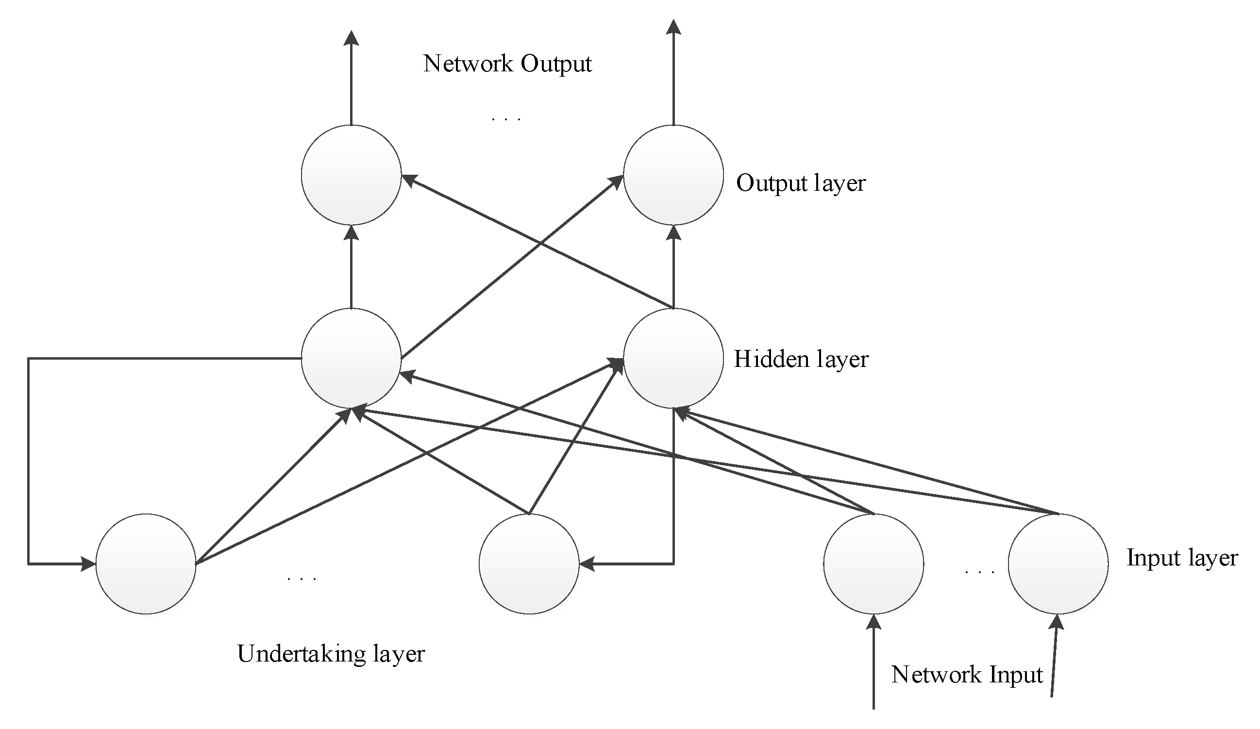
The Elman neural network is a multilayer feedforward neural network and is based on the BP neural network and negative feedback system. BP neural networks generally have an input layer, several hidden layers, and an output layer. In addition, the Elman neural network adds an undertaking layer. Compared with BP neural networks, the Elman neural network has better stability and is better at classifying the original data. The model structure is shown in Figure 9 [24].
The basic mathematical model of an Elman neural network is shown as follow [25]:
x t = f ( w ( 1 ) u t + w ( 2 ) x t ( c ) + b ( h ) )
x t ( c ) = x t 1
Equations (2) and (3) are the calculation expressions of the output values of the hidden layer and input layer of an Elman network, respectively. w(1) the is weight matrix connecting the hidden layer and the input layer, and w(2) is the weight matrix connecting the undertaking layer and the hidden layer. b(h) is the hidden neuron bias vector, and t is the sampling time. xt is the output of hidden layer. x t ( c ) is feedback data.
The excitation function of the Elman neural network is a nonlinear sigmoid function, which is shown in the following formula:
f ( x ) = 1 1 + e x
The output layer neurons of the network are linear transfer functions. The final network output is as follows:
y t = w ( 3 ) x t + b ( 0 )
In this equation, w(3) is the weight matrix connecting the output layer and the hidden layer, b(0) is the output neuron bias vector, and yt is the final network output.
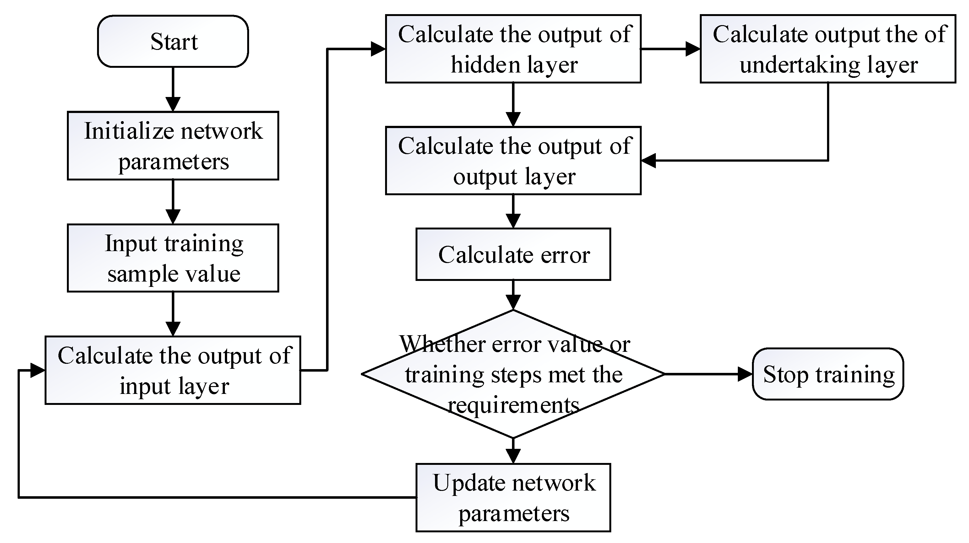
The training process of the Elman neural network is shown in Figure 10.

3.3. The Inverse Model of the MRF Damper

In the inverse model of the MRF damper, the inputs were piston displacement, piston velocity, and damping force, and the output was current. Therefore, the neuron number of input layer m was 3, and the neuron number of the output layer n was 1. The Elman neural network for the neurons number of the hidden layer is generally calculated using the formula b = ( m + n ) + a a∈[1,10], where b is a positive integer. Through multiple trials, the number of neurons in the hidden layer b was 10.
In the network training, the parameters of the Elman neural network, such as learning efficiency, training error, and the number of neurons in each layer, should be initialized first. Then, samples are input to calculate the output and training error of each layer and judge the training error. If the requirements are met or the maximum training times are reached, the training ends. If the requirements are not met, the network parameters are updated and the training continues until the requirements are met or reach the maximum training times. In this training, the target of convergence error was set to 0.001, and the training times was set to 200.
To verify the effectiveness of the Elman neural network, the BP neural network was used to train and predict the MRF damper inverse model, and the prediction results were compared with those of the Elman neural network.
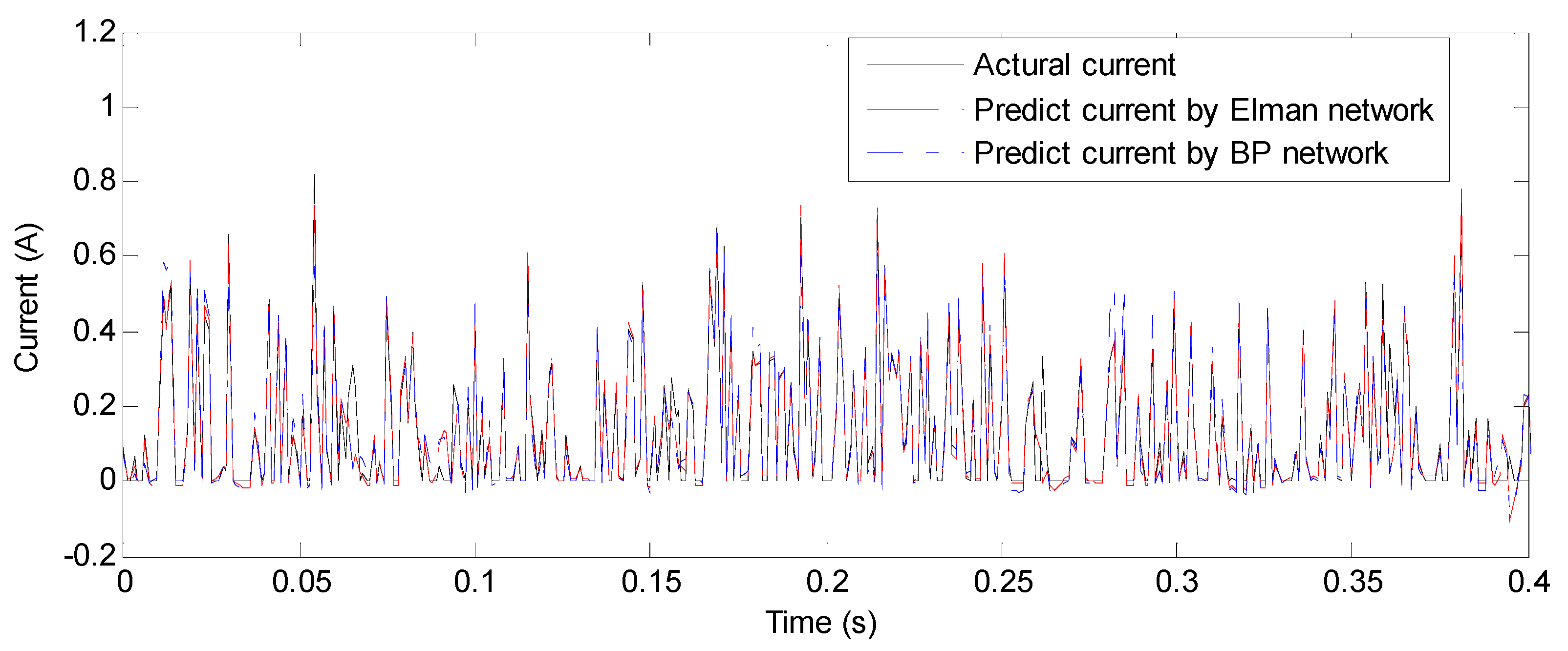
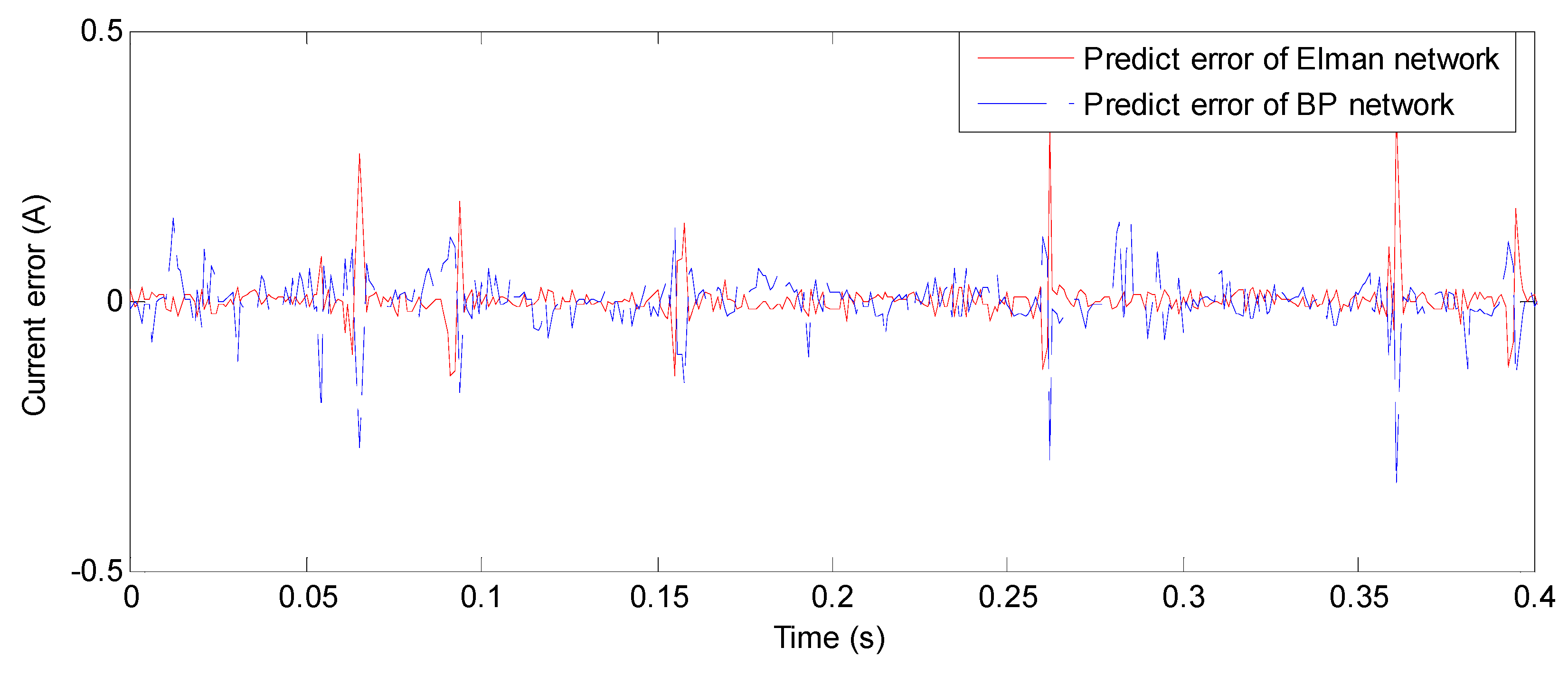
Figure 11 shows the original current and the predicted control current using the Elman and BP neural networks, and Figure 12 shows the error comparison of the control current using the Elman and BP neural networks. From the prediction results and error comparison given in Figure 11 and Figure 12, the fitting effect of the control current predicted by the Elman neural network to the original current sample was higher than that of the BP network, and the root mean square (RMS) value of the Elman neural network prediction error was 0.0236, which was less than that of the BP neural network. The prediction error of BP network was 0.0301. In addition, the fitting error using Elman neural network was reduced by 21.59%, which indicates that the Elman neural network inverse model has better performance.

4. Numerical Simulation of the MRF Suspension

4.1. The Dynamic Model of the Vehicle Suspension

The reverse model of the MRF damper was applied to the semi-active control system of a vehicle suspension model. The system can realize on-line control of vehicle suspension vibration. In the process of vehicle driving, the occupant of the vehicle is excited by vibration in all directions but, generally, the amplitude of vertical vibration is the largest. Therefore, the vertical vibration of the vehicle has great significance for the vehicle ride comfort. Thus, the two degrees of freedom vehicle suspension model, quarter vehicle suspension model, can be used to test the effect of the vehicle semi-active suspension control method for vertical vibration control. It can also be used to verify the control effect of the MRF damper inverse model to achieve continuous adjustable damping. Therefore, this study established a quarter vehicle semi-active suspension model for analysis. The differential equations of vehicle suspension model are shown as follows:
m b x ¨ b + k s ( x b x w ) F d = 0 m w x ¨ w + k s ( x w x b ) + k t ( x w x r ) + F d = 0
where mb is the sprung mass, mw is the unsprung mass, ks is the suspension spring stiffness, kt is the tire stiffness, Fd is the adjustable damping force, in the semi-active control, this force is the sum of the basis damping force (input current is zero) and the semi-active control force, xw is the displacement of the unsprung mass, xb is the displacement of the sprung mass, and xr is the road excitation. The parameters in the system were set as follows: mb = 400 kg, mw = 50 kg, ks = 35,000 N/m, and kt = 200,000 N/m.

4.2. Semi-Active Control Algorithm

As a classical control strategy of the semi-active suspension, the skyhook control method has many advantages such as simple implementation, fewer control variables and easy measurement. The skyhook control strategy is:
f M R F = { c s k y * V r e l       V r e l * V s 0 0                                     V r e l * V s < 0
where csky is the skyhook damping controlled by the current, Vrel is the relative velocity of vehicle suspension (sprung mass velocity minus unsprung mass velocity), and Vs is the sprung mass velocity of vehicle suspension. For traditional skyhook control, the damping force is generated by a fixed current. That is, when the motion of suspension meets the requirements of the output damping force shown in Equation (7), turn on the current switch, input a fixed current, and output the damping force. Otherwise, turn off the current switch and only output the minimum damping force.
However, the skyhook control also has disadvantages: (1) it produces impact load on the suspension system during the damping force switching; (2) the MRF damper can only change between the fixed current and no current under the skyhook control and is thus unable to fully utilize the ability of the MRF damper to adjust damping force continuously and consumes more electric energy. Therefore, a fuzzy algorithm-based skyhook control was examined to maximize the advantage of the MRF damper’s continuously adjustable damping [26].
The input variables of the fuzzy controller were the sprung mass velocity vs. and the relative velocity Vrel, and the output was the damping force factor. This factor was multiplied by the skyhook damping coefficient to obtain the fuzzy control damping coefficient, and then the coefficient was multiplied by Vrel at this moment to obtain the output control force. Based on multiple calculations on the suspension model, the skyhook damping coefficient was selected as 2000 Ns/m.
The input and output of the fuzzy controller must be represented by fuzzy language variables, so the numerical variables should be clear. According to the characteristics of the vehicle suspension system and MRF damper damping force output law, the inputs of Vrel and Vs. were divided into five levels: negative large, negative small, zero, positive small, positive large. These five levels are defined as NB, NS, ZE, PS, and PB, respectively. In addition, the output of fuzzy control was divided into four levels: zero, small, medium, and large. These four levels are defined as ZE, S, M and B, respectively.
The fuzzy logic control rules are based on the skyhook strategy, as shown in Table 3, and the structure of the fuzzy controller is shown in Figure 13.
As shown in Figure 13, the inputs of the fuzzy control were Vrel and Vs, and the discourse domains of the input variables were set as [−1, 1]. The output was set as [0, 1], and then the output was multiplied by the scale factor, Ku, to obtain the fuzzy control output. The control rules and reasoning mechanism of a designed fuzzy controller cannot be adjusted, but the quantization factors Ka and Kv and the scale factor, Ku, can be adjusted, and have significant influence on the controller performance.
At present, many methods exist to select the quantification factors Ka and Kv and the scale factor Ku; however, there is no unified standard. Selection mainly depends on experience. For the semi-active suspension system, it needs to be adjusted repeatedly to achieve a better control effect, which has certain limitations. Therefore, it is necessary to find a feasible and effective method to select quantification factors and scale factors. Because the most important performance index of vehicle suspension is to control the acceleration of the vehicle body, the optimization design method can be used to search for the best quantification factors and scale factors according to the optimization objective and thus obtain the best control effect.
This study used the GWO method to optimize the quantification factors Ka, Kv, and the scale factor Ku, and obtain the best control effect.
The GWO algorithm is a population intelligent optimization method first developed by Mirjalili [27]. The GWO algorithm has the characteristics of simple principle, less calculation requirements. It has been applied in face recognition [27], traffic flow prediction, power system control, and other fields.
The grey wolf population can be divided into four levels: α wolf, β wolf, δ wolf, and ω wolf. The GWO algorithm defines the optimal solution, suboptimal solution, and the third optimal solution as α wolf, β wolf, and δ wolf, which guide hunting; other candidate solutions are defined as ω wolf, which follows α wolf, β wolf, and δ wolf [28]. The predation behavior of grey wolf is divided into encircling, hunting, and attacking. The behavior of wolves surrounding their prey is expressed as [29]:
{ D = | C X p ( t ) X ( t ) |   X ( t + 1 ) = X p ( t ) A D  
where D is the distance between the wolf and its prey; X(t) and Xp(t) are the current positions of the wolf and prey respectively; t is the current number of iterations; A and C are the coefficient vectors.
The specific definitions of A and C are as follows:
{ a = 2 ( 1 t / M )   A = 2 a r a n d 1 a C = 2 r a n d 2  
{ X 1 = X α A 1 D α X 2 = X β A 2 D β X 3 = X δ A 3 D δ
X ( t + 1 ) = ( X 1 + X 2 + X 3 ) / 3
where Dα, Dβ, and Dδ are the distances of the α wolf, β wolf, and δ wolf from the other grey wolves, respectively; Xα, Xβ, and Xδ are the positions of the α wolf, β wolf, and δ wolf, respectively; A1, A2, and A3 are coefficient vectors; C1, C2, and C3 are random vectors; rand1 and rand2 are random vectors in the interval [0, 1], which are generated randomly in the optimization process; X is the position of the current grey wolf individual.
Finally, the wolves attack the prey. The value of the convergence factor a in Formula (8) decreases linearly, and decreases from 2 to 0 with the value of t. When | A | ≤ 1, the wolf pack attacks the prey, highlighting the local search; when A > 1, the wolf pack gives up hunting the current prey and spreads out, highlighting the global search.
The performance of the suspension system has a direct impact on vehicle performance, including ride comfort, handling stability, and ride comfort. Generally, the performance of the suspension system is evaluated based on vertical acceleration, suspension dynamic deflection, roll angle and roll acceleration, pitch angle and pitch acceleration, and tire dynamic load. The vertical displacement and acceleration are usually larger than those in the roll and pitch directions. This study mainly examined the vertical motion caused by the impact when the vehicle is running, and evaluated the suspension performance in terms of the following three aspects: body acceleration, suspension dynamic deflection, and tire dynamic load.
Among the three parameters, the vehicle body acceleration directly represents the vibration intensity transmitted to the vehicle body, which is the most important index to evaluate—the ride comfort of the vehicle. The suspension dynamic deflection affects the probability of hitting the suspension stop; if this parameter is too large, the driving stability of the vehicle will decrease. The tire dynamic load characterizes the ability of the vehicle to resist the road interference; if this parameter is too high, the handling stability of the vehicle will be reduced. In this study, the root mean square (RMS) value of vertical acceleration was chosen as the optimization target. The fitness function is shown as follows:
f fitness = R M S ( a b )
where ab is the vertical acceleration of vehicle body.
After establishing the fitness function, the GWO algorithm was used to optimize the quantification factors Ka, Kv, and the scale factor Ku of fuzzy control. The optimization process was as follows:
(1) Initialization of parameters, which set the optimized parameters of quantification factors Ka, Kv, and the scale factor Ku, had a range of values of [1,10], the maximum number of iterations was 200, and the position of the initialized wolves was X = (X1, X2, …, XN).
(2) Calculate the adaptive function values of each wolf fi (i = 1, 2, …, N), filter the top three grey wolf individuals with adaptive values (α wolf, β wolf, and δ wolf), and determine their locations Xα, Xβ, and Xδ.
(3) The distance between the remaining grey wolf and Xα, Xβ, and Xδ was calculated by Formula (9), and the location of grey wolf α, β, and δ was updated in a timely manner based on Formulas (10) and (11).
(4) Update parameters α, A, and C according to Equation (9).
(5) If the algorithm exceeds the maximum number of iterations, stop the loop and output the optimal solution Xα; otherwise, return to Step (2) to continue the loop.
After the control force is obtained by the optimized fuzzy skyhook method, the semi-active control force is summed with the basic damping force of the MRF damper to obtain the ideal output damping force. Then the ideal output damping force, the relative velocity Vrel, and relative displacement drel are simultaneously updated to the inverse model of the MRF damper to obtain its control current to realize the semi-active control. The control flow is shown in Figure 14.

4.3. Semi-Active Control Simulation

The C class road excitation according to ISO 8608: 2016 [30] was used in this section as shown in Figure 15. The passive vibration reduction method, the traditional skyhook control method, and the optimized fuzzy skyhook method were simulated and compared after optimization using the GWO method. The optimized fuzzy control parameters were Ka = 9.82, Kv = 3.11, and Ku = 1.10. The passive damping method was used such that the current output of the MRF damper was always zero, and the suspension damping could not be changed in the passive vibration reduction state. The traditional skyhook control method used the approach described in Equation (7) to control the vibration.
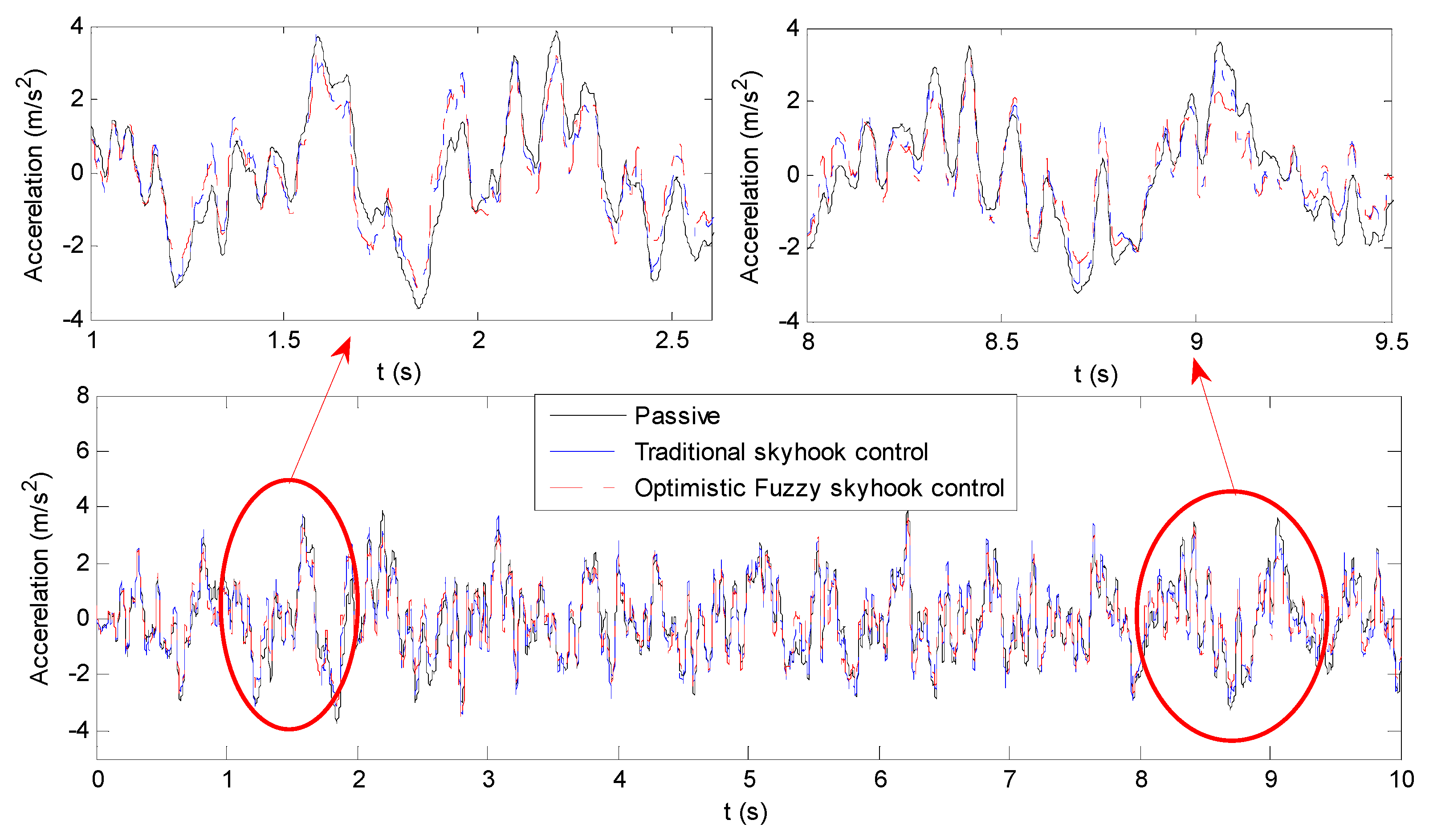
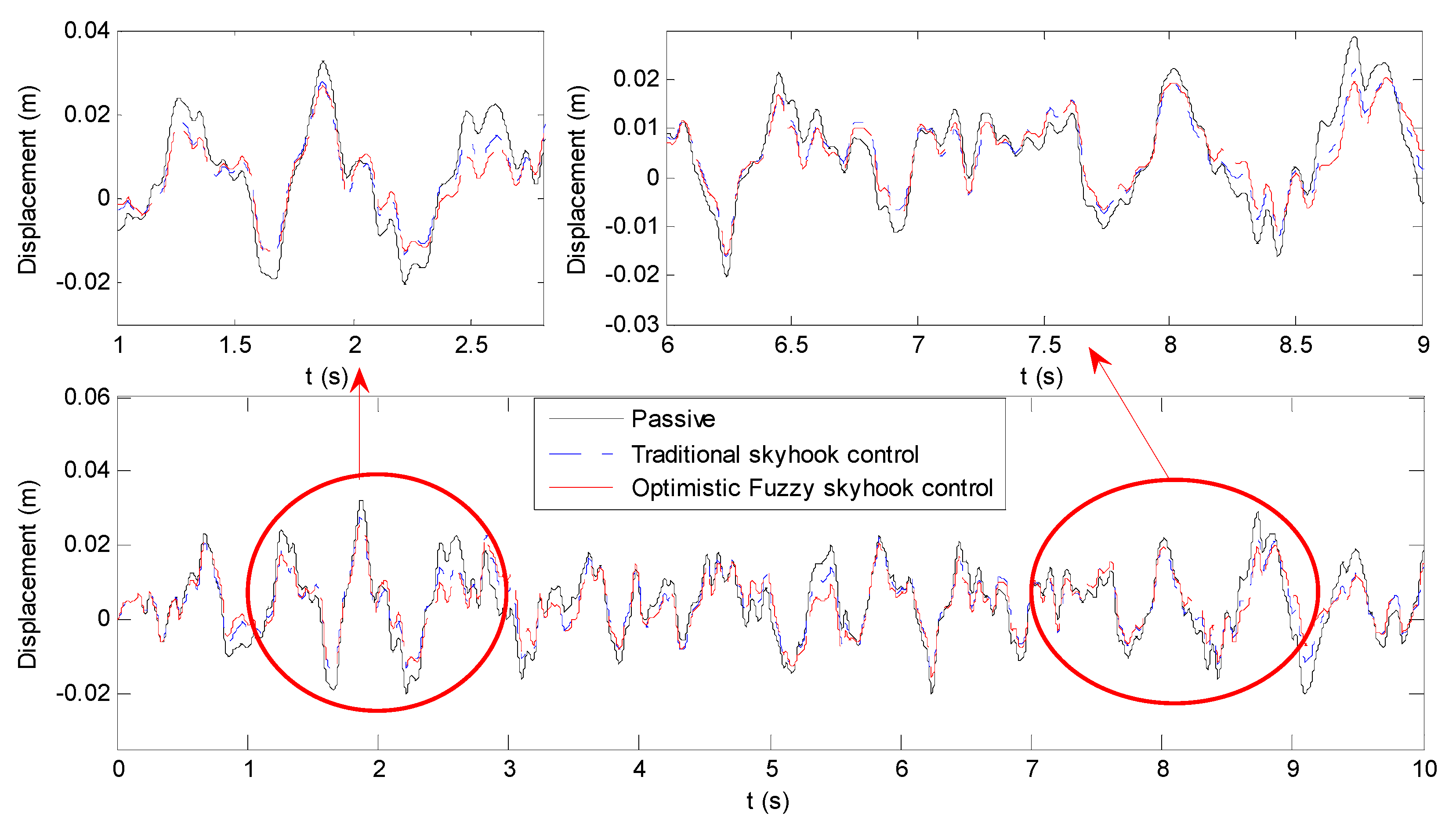
The time histories and RMS values of the vertical acceleration, suspension dynamic deflection, the tire dynamic load under the passive state, the traditional skyhook control, and the GWO fuzzy skyhook control are shown in Table 4 and Figure 16, Figure 17 and Figure 18.
According to the time domain diagrams and RMS values of vertical acceleration, suspension dynamic deflection and tire dynamic load under the three control methods (as shown in Table 3), using traditional skyhook control, the RMS value of vertical acceleration was reduced from 1.3816 to 1.3241 m/s2, the dynamic deflection acceleration was reduced from 0.0111 to 0.0091 m, and tire dynamic load was reduced from 751.1950 to 713.3522 N. This shows that skyhook control can effectively improve suspension performance. After using the fuzzy skyhook control strategy and optimizing the parameters by GWO algorithm, the RMS value of vertical acceleration was further reduced to 1.1864 m/s2, the dynamic deflection was further reduced to 0.0090 m, and the tire dynamic load was further reduced to 705.3631 N. Compared with passive control, these values were reduced by 14.13%, 18.92%, and 6.10%, respectively. This result proves that the optimal control method proposed in this paper was effective.
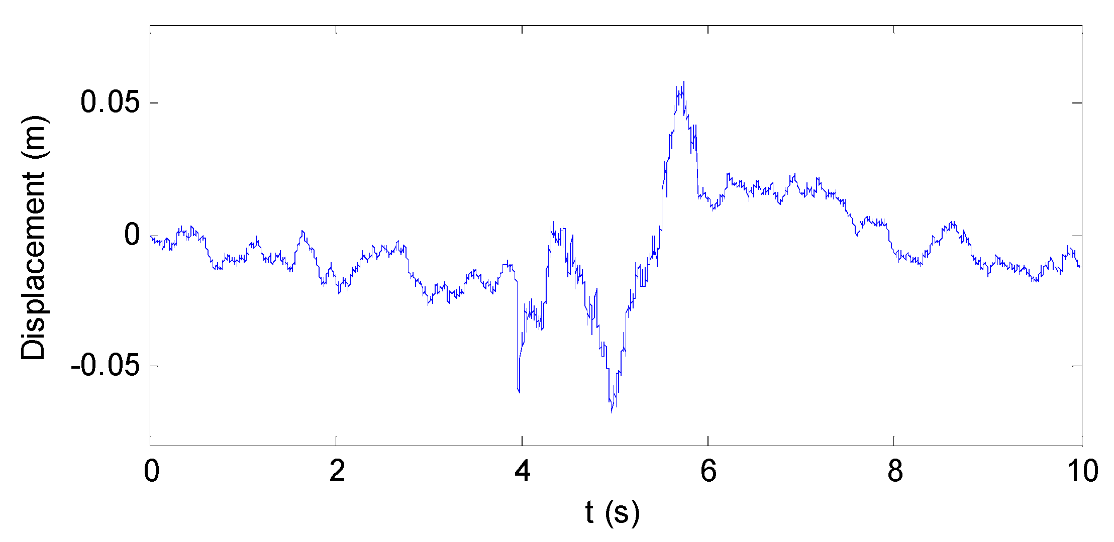
In addition to the normal road surface, driving on a potholed road often results in low-frequency large amplitude shock vibration, which has an adverse impact on vehicle ride comfort. Thus, we also carried out a simulation analysis of the suspension vibration reduction of this condition. This excitation signal is shown in Figure 19.
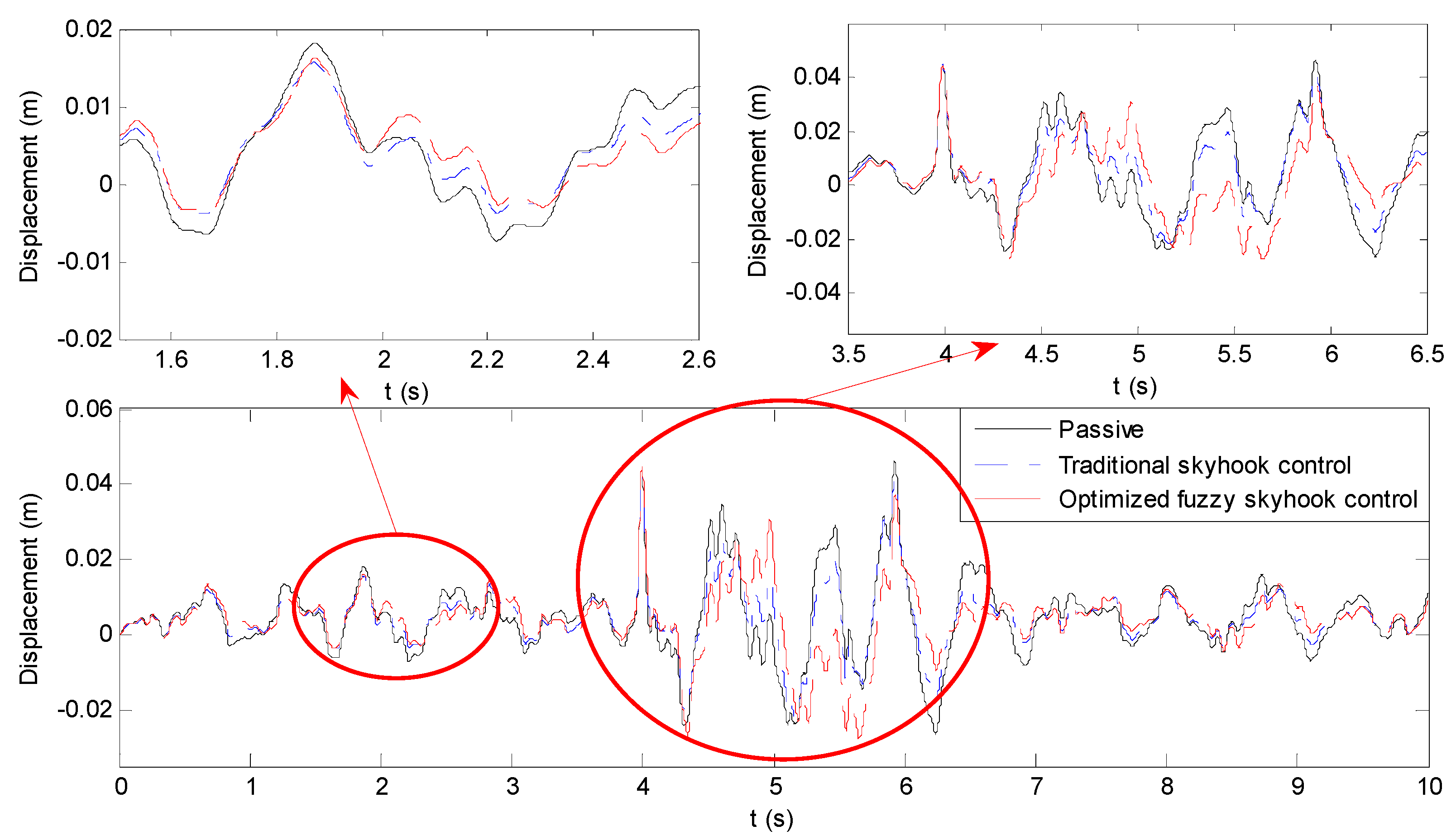
The time histories and RMS values of the body vertical acceleration, suspension dynamic deflection, and tire dynamic using three control methods under potholed road excitation are shown in Table 5 and Figure 20, Figure 21 and Figure 22.
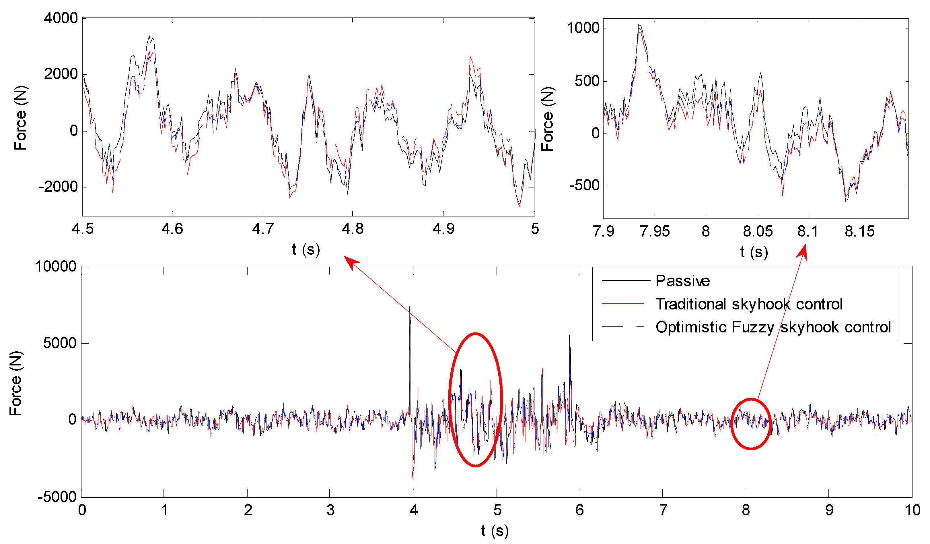
From Table 5 and Figure 20, Figure 21 and Figure 22, it can be seen that under the potholed road condition, using the optimized fuzzy skyhook control strategy, the RMS value of vertical acceleration was reduced from 1.3388 to 1.0356 m/s2, dynamic deflection acceleration was reduced from 0.0110 to 0.0093 m, and tire dynamic load was reduced from 737.9775 to 680.7965 N. Compared with passive control, these values were reduced by 22.65%, 15.46%, and 7.75%, respectively. It can be seen from Figure 20 and Figure 21, that after receiving large amplitude vibration excitation, the optimized fuzzy skyhook control strategy can more quickly lower the acceleration of the vehicle body and decay the dynamic deflection of the suspension. These results prove that the optimal control method proposed in this paper was effective. This shows that the proposed method can also obtain a better damping effect under low-frequency and large amplitude excitation and can improve the ride comfort of vehicles.

5. Conclusions

In this study, the vehicle magnetorheological semi-active suspension with continuously adjustable MRF damping was examined. The inverse model of the MRF damper and the fuzzy skyhook control optimized by the GWO algorithm were investigated through experiment with numerical simulation, aiming to improve the ride comfort and handling stability of the vehicle. The main works are shown as follows:
1. The inverse model of the MRF damper developed using the Elman neural network was established to calculate the control current from the expected output damping force. The inverse model can effectively convert the expected damping force into the control current, and apply the control current to the actual MRF damper to obtain the actual damping force. Thus, the damping force can be continuously adjusted to reduce the suspension vibration. Compared with the BP neural network model, the Elman neural network model reduced the local detail error of the inverse model and improved the prediction accuracy of the control current;
2. A quarter vehicle suspension model was established in which the MRF damper was used for the suspension model, and semi-active control analysis was carried out. The results show that the semi-active vibration control of the MRF damper can effectively improve the ride comfort of the suspension. The vertical vehicle acceleration, suspension dynamic reflection, and tire dynamic load can be reduced simultaneously using the skyhook semi-active control method;
3. A fuzzy skyhook control method based on GWO was proposed, aiming to overcome the shortcomings that the quantification factor and scale factor in the fuzzy control are determined through expert experience. The fuzzy skyhook control method optimized by the GWO algorithm was proposed to optimize the quantification factor and scale factor. The normal road and pothole road conditions were selected for simulation analysis. The analysis results show that this optimized skyhook control method can reduce the vertical acceleration, suspension dynamic reflection, and tire dynamic load. For vertical acceleration, the most important component of the ride comfort index, the control effect of the optimized fuzzy skyhook control method proposed in this paper was clearly better than that of the traditional skyhook control method.
Future research will focus on further improving the semi-active control algorithm to obtain a better damping effect. In addition, the research will be extended to the full-vehicle semi-active suspension system, so that the MRF damper can control the vertical, roll, and pitch vibration of the vehicle simultaneously.

Author Contributions

Writing—original draft, T.M.; Supervision, F.B.; Review and revision, X.W.; methodology, J.L.; software, C.T.; Data curation, J.W., G.P. All authors have read and agreed to the published version of the manuscript.

Funding

This research was funded by the International Cooperation Project for RMIT and Tianjin University Joint Research Center: “Investigation of Low-Frequency Idle Vibration and Lumpiness Control of Commercial Vehicle Driver’s Seat through Passive and Semi-Active Control Technologies”.

Institutional Review Board Statement

Not applicable.

Informed Consent Statement

Not applicable.

Data Availability Statement

Data sharing not applicable.

Conflicts of Interest

The authors declare no conflict of interest.

References

  1. Lloyd John, R.; Hayesmichel Miquel, O.; Radcliffe Clark, J. Internal Organizational Measurement for Control of Magnetorheological Fluid Properties. J. Fluids Eng. 2007, 129, 4. [Google Scholar] [CrossRef]
  2. Lee, C.-H.; Jang, M.-G. Virtual Surface Characteristics of a Tactile Display Using Magneto-Rheological Fluids. Sensors 2011, 11, 2845–2856. [Google Scholar] [CrossRef] [PubMed] [Green Version]
  3. Du, H.; Lam, J.; Cheung, K.C.; Li, W.; Zhang, N. Direct voltage control of magnetorheological damper for vehicle suspensions. Smart Mater. Struct. 2013, 22, 105016. [Google Scholar] [CrossRef]
  4. Wang, J.; Dong, C.; Shen, Y.; Wei, J. Robust modelling and control of vehicle active suspension with MR damper. Veh. Syst. Dyn. 2011, 46, 509–520. [Google Scholar] [CrossRef]
  5. Liu, Z.; Ren, H.; Chen, S.; Chen, Y.; Feng, J. Feedback Linearization Kalman Observer Based Sliding Mode Control for Semi-Active Suspension Systems. IEEE Access 2020, 8, 71721–71738. [Google Scholar] [CrossRef]
  6. Esteki, K.; Bagchi, A.; Sedaghati, R. Dynamic analysis of electro- and magneto-rheological fluid dampers using duct flow models. Smart Mater. Struct. 2014, 23, 035016. [Google Scholar] [CrossRef]
  7. Bouc, R. A Mathematical Model for Hysteresis. Acta Acust. United Acust. 1971, 24, 16–25. [Google Scholar]
  8. Wen, Y.K. Method of random vibration of hysteretic systems. J. Eng. Mech. 1976, 102, 249–263. [Google Scholar]
  9. Stanway, R.; Sproston, J.L.; Stevens, N.G. Non-linear modelling of an electro-rheological vibration damper. J. Electrost. 1987, 20, 167–184. [Google Scholar] [CrossRef]
  10. Dahl, P.R. Solid Friction Damping of Mechanical Vibrations. AIAA J. 2012, 14, 1675–1682. [Google Scholar] [CrossRef]
  11. Hiwatashi, T.; Shiozaki, Y.; Fujitani, H.; Minowa, C.; Soda, S. Shaking table tests on semi-active base-isolation system by magnetorheological fluid damper. In Proceedings Volume 5056, Smart Structures and Materials 2003: Smart Structures and Integrated Systems, Proceedings of the Smart Structures and Materials, San Diego, CA, USA, 2–6 March 2003; SPIE: Bellingham, WA, USA, 2012; Volume 14. [Google Scholar]
  12. Qian, L.J.; Liu, B.; Chen, P.; Bai, X.X. An inverse model for magnetorheological dampers based on a restructured phenomenological model. In Proceedings Volume 9799, Active and Passive Smart Structures and Integrated Systems, Proceedings of the 2016 SPIE Smart Structures and Materials + Nondestructive Evaluation and Health Monitoring, Las Vegas, NV, USA, 20–24 March 2016; SPIE: Bellingham, WA, USA, 2013; Volume 14. [Google Scholar]
  13. Liu, X.; Wang, N.; Wang, K.; Chen, S.-M.; Sun, S.; Li, Z.; Li, W. A new AI-surrogate model for dynamics analysis of a magnetorheological damper in the semi-active seat suspension. Smart Mater. Struct. 2020, 29, 037001. [Google Scholar] [CrossRef]
  14. Dzung, N.S.; Choi, S.B. A new neuro-fuzzy training algorithm for identifying dynamic characteristics of smart dampers. Smart Mater. Struct. 2012, 21, 85021. [Google Scholar]
  15. Zhang, N.; Zhao, Q. Fuzzy sliding mode controller design for semi-active seat suspension with neuro-inverse dynamics approximation for MR damper. J. Vibroengineering 2017, 19, 3488–3511. [Google Scholar]
  16. Lv, J.; Guo, C.; Shen, Z.P.; Zhao, M.; Zhang, Y. Summary of Artificial Neuron Model Research. In Proceedings of the IECON 2007-33rd Annual Conference of the IEEE Industrial Electronics Society, Taipei, Taiwan, 5–8 November 2007. [Google Scholar]
  17. Wang, X.; Bi, F.; Du, H. Reduction of low frequency vibration of truck driver and seating system through system parameter identification, sensitivity analysis and active control. Mech. Syst. Signal Process. 2017, 105, 16–35. [Google Scholar] [CrossRef]
  18. Bi, F.; Ma, T.; Wang, X. Research on Vibration Control of Seating System Platform Based on the Cubic Stewart Parallel Mechanism. IEEE Access 2019, 7, 155637–155649. [Google Scholar] [CrossRef]
  19. Weber, F. Robust force tracking control scheme for MR dampers. Struct. Control Health Monit. 2015, 22, 1373–1395. [Google Scholar] [CrossRef]
  20. Weber, F. Semi-active vibration absorber based on real-time controlled MR damper. Mech. Syst. Signal Process. 2014, 46, 272–288. [Google Scholar] [CrossRef]
  21. Yu, M. Study on MR Semi-active Suspension System and its Road Testing. J. Intell. Mater. Syst. Struct. 2006, 17, 801–806. [Google Scholar] [CrossRef]
  22. Sulaiman, M.H.; Mustaffa, Z.; Mohamed, M.R.; Aliman, O. Using the gray wolf optimizer for solving optimal reactive power dispatch problem. Appl. Soft Comput. 2015, 32, 286–292. [Google Scholar] [CrossRef] [Green Version]
  23. Peng, G.R.; Li, W.H.; Du, H. Modelling and identifying the parameters of a magneto-rheological damper with a force-lag phenomenon. Appl. Math. Model. 2015, 38, 3763–3773. [Google Scholar] [CrossRef]
  24. Wang, J. A deep learning approach for atrial fibrillation signals classification based on convolutional and modified Elman neural network. Future Gener. Comput. Syst. 2019, 102, 670–679. [Google Scholar] [CrossRef]
  25. Yaoli, W.; Lipo, W.; Fangjun, Y.; Wenxia, D.; Qing, C. Advantages of direct input-to-output connections in neural networks: The Elman network for stock index forecasting. Inf. Sci. 2021, 547, 1066–1079. [Google Scholar]
  26. Sun, S.S.; Ning, D.H.; Yang, J.; Du, H.; Zhang, S.W.; Li, W.H. A seat suspension with a rotary magnetorheological damper for heavy duty vehicles. Smart Mater. Struct. 2016, 25, 105032. [Google Scholar] [CrossRef]
  27. Mirjalili, S.; Mirjalili, S.M.; Lewis, A. Grey wolf optimizer. Adv. Eng. Softw. 2014, 69, 46–61. [Google Scholar] [CrossRef] [Green Version]
  28. Huang, X.; Huang, X.; Wang, B.; Xie, Z. Fault diagnosis of transformer based on modified grey wolf optimization algorithm and support vector machine. IEEJ Trans. Electr. Electron. Eng. 2020, 15, 409–417. [Google Scholar] [CrossRef]
  29. Li, S.; Wang, F. Research on Optimization of Improved Gray Wolf Optimization-Extreme Learning Machine Algorithm in Vehicle Route Planning. Discret. Dyn. Nat. Soc. 2020, 2020, 1–7. [Google Scholar] [CrossRef]
  30. ISO 8608: 2016 Mechanical Vibration–Road Surface Profiles–Reporting of Measured Data; International Organization for Standardization: Geneva, Switzerland, 2016.
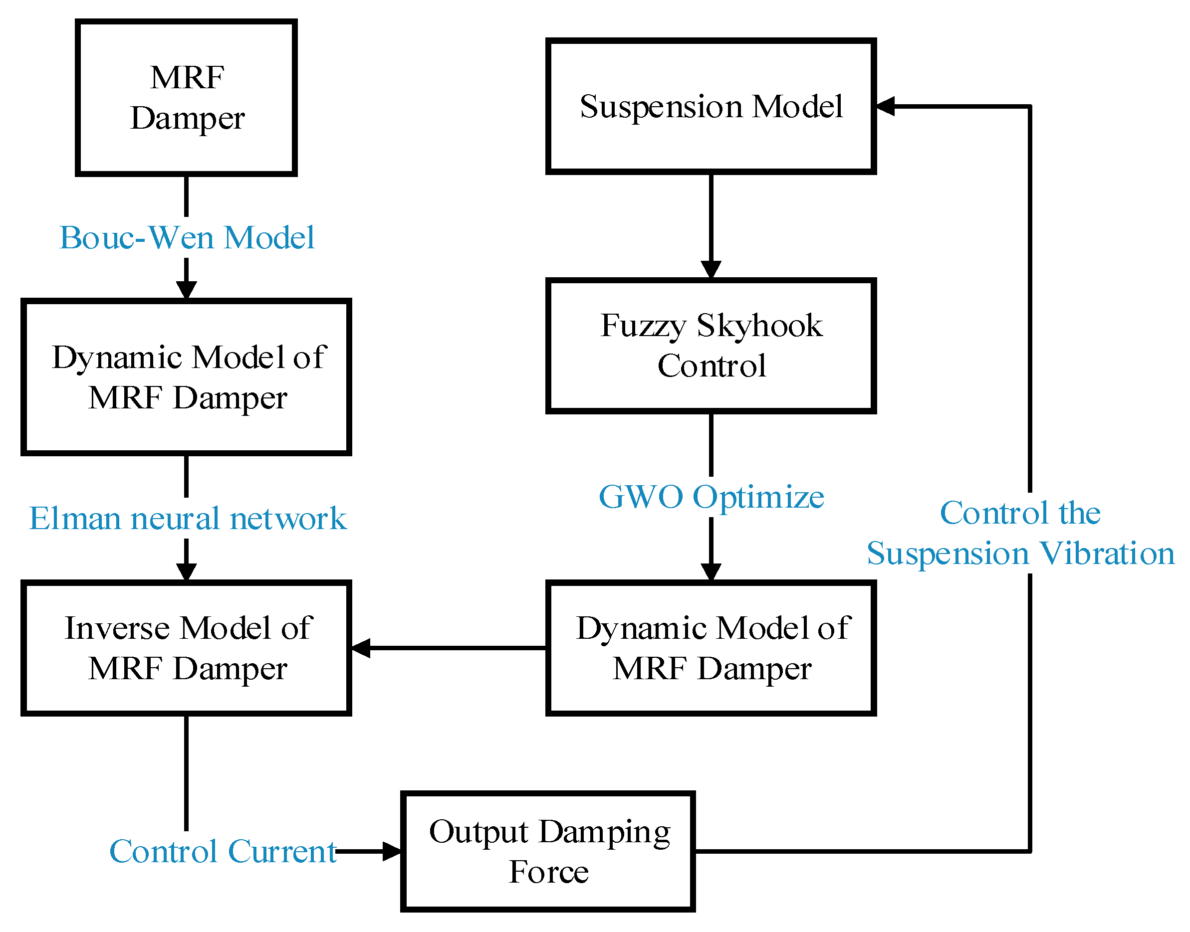
Figure 1. The schematic of the research workflow.
Energies 14 01674 g001
Figure 2. The structure of magnetorheological damper.
Energies 14 01674 g002
Figure 3. Damping characteristics test of the magnetorheological fluid damper. (a) Instron E10000 electronic dynamic testing machine; (b) MRF damper installed on the dynamic testing machine.
Energies 14 01674 g003
Figure 4. Damping characteristic diagram of the MRF damper (a): the displacement–force characteristic curves for different control currents under the harmonic excitation of 5 mm amplitude and 1 Hz frequency; (b) the velocity−force characteristic curves for different control currents under the harmonic excitation of 5 mm amplitude and 1 Hz frequency.
Energies 14 01674 g004
Figure 5. Damping characteristics test of the MRF damper: (a) Bouc-Wen model structure; (b) the relationship between the damping force, F, and relative velocity, v, of the MRF damper.
Energies 14 01674 g005
Figure 6. Damping characteristics test of the MRF damper.
Energies 14 01674 g006
Figure 7. Comparisons of the simulation results with experimental results: (a) the displacement−force characteristic curves for different control currents under the harmonic excitation of 5 mm 1 Hz; (b) the velocity−force characteristic curves for different control currents under the harmonic excitation of 5 mm 1 Hz.
Energies 14 01674 g007
Figure 8. Comparisons of the simulation results with the experimental results: (a) force−displacement and (b) force−velocity under 0.5 Hz sinusoidal excitation of 10 mm amplitude for a control current of 0.25 A.
Energies 14 01674 g008
Figure 9. The model structure of Elman neural network.
Energies 14 01674 g009
Figure 10. Elman neural network training process.
Energies 14 01674 g010
Figure 11. The predicted values of the current using the Elman and back propagation (BP) networks.
Energies 14 01674 g011
Figure 12. Current errors using the Elman and BP networks.
Energies 14 01674 g012
Figure 13. Structure of the fuzzy controller.
Energies 14 01674 g013
Figure 14. Control process of the semi-active suspension.
Energies 14 01674 g014
Figure 15. Road excitation of the C Class road profile.
Energies 14 01674 g015
Figure 16. Comparison of the body vertical acceleration of the three control methods under C class road excitation.
Energies 14 01674 g016
Figure 17. Comparison of the suspension dynamic deflections using the three control methods under C class road excitation.
Energies 14 01674 g017
Figure 18. Comparison of the tire dynamic loads using the three control methods under C class road excitation.
Energies 14 01674 g018
Figure 19. Potholed road excitation simulation signal.
Energies 14 01674 g019
Figure 20. Comparison of the body vertical acceleration using the three control methods under potholed road excitation.
Energies 14 01674 g020
Figure 21. Comparison of the suspension dynamic deflections using the three control methods under potholed road excitation.
Energies 14 01674 g021
Figure 22. Comparison of the tire dynamic loads of using the three control methods under potholed road excitation.
Energies 14 01674 g022
Table 1. Initial values of Bouc-Wen model parameters.
Parametersc0 (N.s/mm)βγnk0 (N/mm)x0 (mm)Aα
Value1111110050100
Table 2. Identification result of Bouc-Wen model parameters.
ParametersValue
c0 (N.s/mm)1.87 I + 3.62
β0.0071
γ35.941
n1.0013
k0 (N/mm)2.991
x0 (mm)58.362
A−18.03 I2 + 47.3 I + 41.96
α−15.35 I2 + 46.26 I + 42.56
Table 3. Rules of the fuzzy controller.
Vrel
VsNBNSZEPSPB
NBBMSZEZE
NSMSZEZEZE
ZESZEZEZES
PSZEZEZESM
PBZEZESMB
Table 4. Body vertical root mean square (RMS) acceleration, suspension dynamic deflection, and tire dynamic load under C class road excitation.
RMS ValuePassiveTraditional Skyhook ControlGWO Fuzzy Skyhook Control
Vertical acceleration (m/s2)1.38161.32411.1846
Suspension dynamic deflection (m)0.01110.00910.0090
Tire dynamic load (N)751.1950713.3522705.3631
Table 5. Body vertical RMS acceleration, the suspension dynamic deflection, and the tire dynamic load under potholed road excitation.
RMS ValuePassiveTraditional Skyhook ControlGWO Fuzzy Skyhook Control
Vertical acceleration (m/s2)1.33881.23521.0356
Suspension dynamic deflection (m)0.01100.00920.0093
Tire dynamic load (N)737.9775695.6184680.7965
Publisher’s Note: MDPI stays neutral with regard to jurisdictional claims in published maps and institutional affiliations.