An Immersed Boundary Method Based Improved Divergence-Free-Condition Compensated Coupled Framework for Solving the Flow–Particle Interactions

Abstract

A flow–particle interaction solver was developed in this study. For the basic flow solver, an improved divergence-free-condition compensated coupled (IDFC²) framework was employed to predict the velocity and pressure field. In order to model the effect of solid particles, the differentially interpolated direct forcing immersed boundary (DIIB) method was incorporated with the IDFC² framework, while the equation of motion was solved to predict the displacement, rotation and velocity of the particle. The hydrodynamic force and torque which appeared in the equations of motion were directly evaluated by fluid velocity and pressure, so as to eliminate the instability problem of the density ratio close to 1. In order to effectively evaluate the drag/lift forces acting on the particle, an interpolated kernel function was introduced. The present results will be compared with the benchmark solutions to validate the present flow–particle interaction solver.

1. Introduction

The offshore wind farm is a wind turbine installed in an offshore area where there is a strong wind field for a long period of time. It can avoid the noise, shading and visual obstruction caused by the wind turbine’s operation in the land area. Offshore wind farms can also provide more stable wind energy and low turbulence effects. However, it requires consideration of the effects of wind turbulence on the wind turbine and its supporting structure. Recently, attention has also been paid to the offshore floating wind turbine. How to efficiently simulate the interaction between the floating structure and the water/air interface becomes an important research topic.

The coupling analysis of fluids and solids in practical engineering applications usually requires the consideration of complex geometries. These complex geometries are usually in a stationary or transient motion at high Reynolds number flows, such as offshore stationary wind turbines and marine systems. These fluid–structure problems are typically solved by the traditional body-fitted-grid. In order to generate high-quality mesh, a lot of efforts in terms of manpower are always required to refine the mesh at the high curvature region. The computational cost is then increased, especially when dealing with the moving boundary problems. In addition, the quality of the grid is also very crucial for simulation analysis.

In recent decades, the immersed boundary method has been shown to have great potential for modeling the flow–particle interaction problem. It is achieved by virtue of incorporating introduced momentum forcing terms in the equations of motion to predict the displacement, rotation and velocity of the solid object [1]. The main advantage of employing an immersed boundary method for this kind of problem is that the regular fixed Cartesian grid can still be used for simulating the complex time-varying geometries.

However, how to effectively evaluate the drag/lift of the coupling interface and the particle velocity is still a research topic to be refined. Uhlmann [2] proposed incorporating the regularized delta function approach to model the particulate flows, and the improved methods were then proposed by Kempe and Fröhlich [3] and Breugem [4]. Zhang and Gay [5] also proposed a finite element method based on an immersed boundary for fluid–structure interactions. Alternatively, Luo et al. [6] simulated the fluid–particle interactions by direct-forcing based modified immersed boundary method. To further improve the accuracy of velocity in moving solid, Wang et al. [7] introduced the multi-direct forcing method. Yang and Stern [8] also demonstrated a sharp interface-based immersed boundary method by virtue of the direct-forcing approach for solving particulate flows, while Horng et al. [9] exhibited a prediction-correction based direct-forcing immersed boundary projection method for solving fluid–particle interactions.

With the success of finite volume and finite element frameworks, scientists are also motivated to employ an immersed boundary based fluid–particle solver on the Lattice–Boltzmann (LB) framework. Wu and Shu [10] demonstrated a boundary condition-enforced immersed boundary LB scheme to solve particulate flows, while Hao and Zhu [11] revealed an implicit immersed boundary method on the Lattice–Boltzmann framework for fluid–structure interactions. Wang et al. [12] later evaluated three LB schemes to understand their performance when modeling the particulate flows. Zhou and Fan [13] also presented a LB immersed boundary scheme based on the work of Breugem [4]. Zhang et al. [14] further exhibited the particulate immersed boundary method (PIBM) to speed up the calculation of the particulate flow simulations. Coclite et al. [15] proposed kinematic and dynamic forcing strategies for predicting the transport of inertial capsules, and later extend to model the deformable inertial capsules [16].

Due to the fact that the convergence of the Lattice-Boltzmann framework is based on equilibrium equations, each fluid must have its own balance equation for the convergence of the Lattice–Boltzmann method. Furthermore, the definitions of boundary conditions in the Lattice–Boltzmann method is still developing for fitting the physical properties of interfaces. Moreover, some previous studies still only applied the prescribed motion of solid particle for the fluid–solid interaction simulation.

To alleviate the issue of evaluating drag and lift forces, Chiu and Poh [17] have recently successfully incorporated the improved divergence-free-condition compensated coupled (IDFC²) framework with the direct forcing immersed boundary (DIIB) method [18] for solving the flows with prescribed-motion time-varying geometries. The spurious force oscillation (SFO) can be efficiently alleviated and the calculation is relatively simple. This motivated us to incorporate the IDFC² framework with equation of particle motion for simulating the fluid–particle interactions. The ultimate goal for this study is to develop the solver to model the interaction between the floating wind turbine and water/air interface.

In this study, the framework will be extended for simulating the fluid–particle interactions. To prevent the instability problem when the density ratio is close to 1, the drag and lift forces will be directly evaluated from fluid velocity and pressure. An interpolated kernel function to accurately and effectively evaluate the drag/lift forces will be proposed. Details of calculating the equation of motion as well as near-wall treatment when the solid particle is approaching the wall will also be addressed.

This paper is organized as follows. Section 2 presents the governing equations for fluid flows and solid particles. Section 3 present the DIIB method and the methodology for fluid–particle interactions. Section 4 presents the IDFC² based flow–particle interaction framework. Verification studies are presented in Section 5. This is followed by presenting the simulated results to show the applicability for the proposed framework. Finally, some concluding remarks are drawn in Section 6.

2. Governing Equations

2.1. Incompressible Navier–Stokes Equations

The non-dimensional primitive-variable Navier–Stokes equations for incompressible flows can be expressed as the following momentum equations and continuity equation:

$$\frac{\partial \stackrel{\rightharpoonup }{u}}{\partial t}+\nabla ·\left(\stackrel{\rightharpoonup }{u}\stackrel{\rightharpoonup }{u}\right)=\frac{1}{Re}{\nabla }^2\stackrel{\rightharpoonup }{u}-\nabla p+\stackrel{\rightharpoonup }{f}$$

(1)

$$\nabla ·\stackrel{\rightharpoonup }{u}=0$$

(2)

where $\stackrel{\rightharpoonup }{u}$ is the velocity vector, $p$ is the pressure field, and $Re$ is the Reynolds number. $\stackrel{\rightharpoonup }{f}$ is external force vectors due to particle motions, and is modeled by the present immersed boundary based flow–particle interaction framework.

2.2. Equations of Motion for Solid Particle

The equations of motion for the rigid body can be written as

$${\rho }_S{V}_s\frac{d\stackrel{\rightharpoonup }{U}}{dt}=({\rho }_S-{\rho }_f)V_s\stackrel{\rightharpoonup }{g}+\stackrel{\rightharpoonup }{F_f}$$

(3)

$$\frac{d\stackrel{\rightharpoonup }{X}}{dt}=\stackrel{\rightharpoonup }{U}$$

(4)

$$I_S\frac{d\stackrel{\rightharpoonup }{\omega }}{dt}=\stackrel{\rightharpoonup }{{\psi }_f}$$

(5)

$$\frac{d\stackrel{\rightharpoonup }{\mathsf{\Omega }}}{dt}=\stackrel{\rightharpoonup }{\omega }$$

(6)

where the linear velocity vector ($\stackrel{\rightharpoonup }{V})$ and particle position vector ($\stackrel{\rightharpoonup }{X}$) are due to linear motion, while $\omega$ and $\mathsf{\Omega }$ are the angular velocity and orientation due to the angular motion. ${\rho }_S$ and ${\rho }_f$ are the density for the solid particle and fluid, respectively. $V_s$ is the volume of the solid particle, $\stackrel{\rightharpoonup }{g}$ is the gravity, and $I_S$ is the inertial moment of the solid particle. $\stackrel{\rightharpoonup }{F_f}$ and $\stackrel{\rightharpoonup }{{\psi }_f}$ are the hydrodynamic force and torque acting on the solid particle, respectively.

As stated in [2,3], when we evaluated the $\stackrel{\rightharpoonup }{F_f}$ and $\stackrel{\rightharpoonup }{{\psi }_f}$ by the summation of forcing terms $\stackrel{\rightharpoonup }{f}$ together with the relation of momentum balance over the corresponding fluid domain [2], it will lead to an instability issue when the density ratio close to 1, or $({\rho }_S-{\rho }_f)\approx 0$. This is due to the fact that the term $({\rho }_S-{\rho }_f)$ will appear in the denominator when solving the equations of motion. In order to avoid this issue, hydrodynamic force and torque are directly evaluated in this study:

$$\stackrel{\rightharpoonup }{F_f}={\rho }_f{{\displaystyle \int }}^{ }\underset{\_}{\underset{\_}{\sigma }}·n dA$$

(7)

$$\stackrel{\rightharpoonup }{{\psi }_f}={\rho }_f{{\displaystyle \int }}^{ }r\times (\underset{\_}{\underset{\_}{\sigma }}·n) dA$$

(8)

It is noted that by using the present approach, $({\rho }_S-{\rho }_f)$ will be never appear in the denominator, so that there will be no instability problems even when the density ratio id close to 1. In Section 3.1, the present study will introduce methods to accurately and effectively evaluate the two above equations. Furthermore, the implicit midpoint temporal scheme was employed to solve Equations (3)–(6) in the present study.

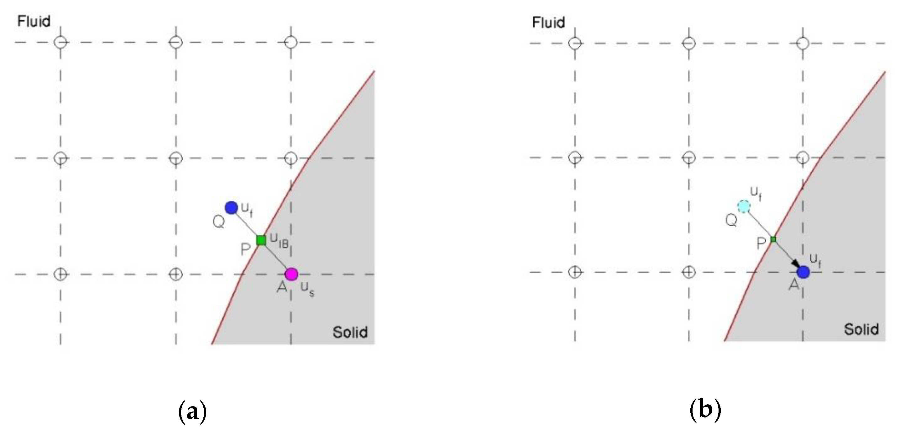
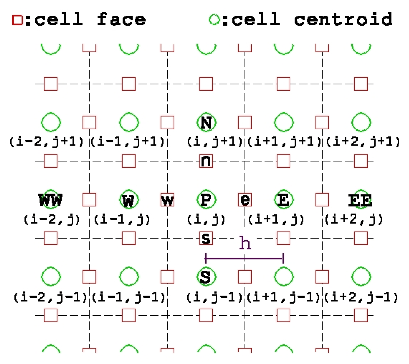
3. Differentially Interpolated Direct Forcing Immersed Boundary (DIIB) Method

In this section, the DIIB method is employed to model the solid body. Here, we will briefly describe the fundamental idea of the DIIB method.

Assuming there is a solid object $S$ immersed in the Eulerian grid; in order to model the effect of solid object, the direct forcing term $\stackrel{\rightharpoonup }{f}$ is introduced in Equation (1) to satisfy the velocity condition ($\stackrel{\rightharpoonup }{V}$) of the solid object. With the semi-implicit discretization, Equation (1) can be split into the following two equations:

$$\frac{{\stackrel{\rightharpoonup }{u}}^{*}-{\stackrel{\rightharpoonup }{u}}^n}{\Delta t}=-\nabla ·{\left(\stackrel{\rightharpoonup }{u}\stackrel{\rightharpoonup }{u}\right)}^{*}=\frac{1}{Re}{\nabla }^2{\stackrel{\rightharpoonup }{u}}^{*}-\nabla p$$

(9)

$$\frac{\stackrel{\rightharpoonup }{V}-{\stackrel{\rightharpoonup }{u}}^{*}}{\Delta t}=\stackrel{\rightharpoonup }{f}$$

(10)

It is noted that in practice, the boundary points of the solid object do not always fall into the Eulerian grid points. The direct forcing method will then evaluate the modified velocity on some target Eulerian grid points, followed by obtaining the corresponding momentum forcing terms based on Equation (10) to model the effect of solid object with velocity condition $\stackrel{\rightharpoonup }{V}$.

For the DIIB method, the velocity ($u_S$) at Eulerian grid point which is inside and close to the solid boundary, will be modified to satisfy the velocity condition $u_{IB}$ at the solid boundary by virtue of interpolated velocity at fluid domain $u_f$ and Taylor series expansion:

$$u_S=2u_{IB}-u_f$$

(11)

Taking Figure 1 as an example, in general $u_F$ does not always lie on the grid point. The evaluation of $u_f$ is done by “advect” $u_f$ from point Q to point A [18]:

$$\frac{\partial u_f}{\partial \tau }+\left(\stackrel{\rightharpoonup }{n}·\nabla \right)u_f=0$$

(12)

In the above, $\stackrel{\rightharpoonup }{n}$ is the unit normal vector of the solid object. In practice, Equation (12) is solved by first order upwind with single artificial time step $\Delta \tau =\overline{APQ}/\left|\stackrel{\rightharpoonup }{n}\right|=2\overline{AP}/\left|\stackrel{\rightharpoonup }{n}\right|$. The reader can refer to [18] for details.

To alleviate the spurious force oscillations (SFOs) and to obtain smooth pressure, the velocity modification method [17] was employed in this study. The idea behind this method is to modify the velocity inside the velocity to the solid object moving velocity when solving the pressure correction equation. It has been shown in [17] that this method successfully suppresses the SFO for the problems with prescribed motions and will then be implemented for dealing with the problem for which the motions are obtained by solving equations of motion.

3.1. Evaluation of Drag and Lift Forces

When employing the direct forcing immersed boundary method, it is suggested to evaluate forces $\underset{\_}{F}$ by the following equation for calculating drag and lift forces:

$$\underset{\_}{F}={{\displaystyle \int }}^{ }\underset{\_}{\underset{\_}{\sigma }}·n dA$$

(13)

where $\underset{\_}{\underset{\_}{\sigma }}$ is the summation of shear and pressure stress, $n$ is unit normal vector and $A$ is surface area. In this study, a four-point piecewise discrete delta function based interpolated kernel is employed [17]:

$$F\left(X,Y\right)={{\displaystyle \sum }}^{ }F\left(x,y\right){\varphi }^{\prime }\left(\frac{x-X}{h}\right){\varphi }^{\prime }\left(\frac{y-Y}{h}\right)$$

(14)

$${\varphi }^{\prime }\left(\frac{x-X}{h}\right)=\varphi \left(\frac{x-X}{h}\right)/{{\displaystyle \sum }}^{ }\varphi \left(\frac{x-X}{h}\right)$$

(15)

$${\varphi }^{\prime }\left(\frac{y-Y}{h}\right)=\varphi \left(\frac{y-Y}{h}\right)/{{\displaystyle \sum }}^{ }\varphi \left(\frac{y-Y}{h}\right)$$

(16)

$$\varphi \left(r\right)=\{\begin{array}{c}\frac{1}{8}\left(3-2\left|r\right|+\sqrt{1+4\left|r\right|+4r^2}\right), \left|r\right|\le 1\\ \frac{1}{8}\left(5-2\left|r\right|-\sqrt{-7+12\left|r\right|-4r^2}\right) ,1\le \left|r\right|\le 2\\ 0 , \left|r\right|\ge 2 \end{array}$$

(17)

when the solid particle is approaching the wall, the interpolated kernel will be simplified to the following one-point piecewise discrete delta function [19]:

$$\varphi \left(r\right)\{\begin{array}{c}1-\left|r\right|, \left|r\right|\le 1\\ 0 , \left|r\right|\ge 1\end{array}$$

(18)

4. Improved Divergence-Free-Condition Compensated Coupled (IDFC²) Framework

The idea behind the IDFC² framework is to discretize momentum equations by virtue of cell-center and cell-face velocity [17]. With the present approach, we can not only obtain the accurate velocity vector $\left(u,v\right)$, but also the fully coupled pressure field $p$. The following will first introduce the original IDFC framework, then briefly describe how to mitigate to IDFC² framework.

4.1. Derivation of IDFC Framework

With the 2D grid structure as shown in Figure 2, the derivation of the IDFC framework starts from the semi-discrete momentum equation. Without loss of generality, we take velocity $u$ at the cell-center P ($u_p$) as an example:

$$\frac{u_P^{*}-u_P^n}{\Delta t}+{(\frac{\partial uu}{\partial x})}_P+{(\frac{\partial vu}{\partial y})}_P=\frac{1}{Re}{(\frac{{\partial }^{2}u}{\partial x^2}+\frac{{\partial }^{2}u}{\partial y^2})}_P-{(\frac{\partial p^n}{\partial x})}_P$$

(19)

The idea for the IDFC method is that discretizing the momentum equation for the cell-face $u_e$ should have the same form as we discretize the momentum equation at the cell-center:

$$\frac{u_e^{*}-u_e^n}{\Delta t}+{(\frac{\partial uu}{\partial x})}_e+{(\frac{\partial vu}{\partial y})}_e=\frac{1}{Re}{(\frac{{\partial }^{2}u}{\partial x^2}+\frac{{\partial }^{2}u}{\partial y^2})}_e-{(\frac{\partial p^n}{\partial x})}_e$$

(20)

However, obtaining the velocity derivatives on the cell-face is not as easy as on the cell-center. The linear-averaged approximation is then employed to evaluate the cell-face velocity derivatives on the cell-face $e$ [20]:

$${(\frac{\partial uu}{\partial x})}_e\approx {(\widehat{\frac{\partial uu}{\partial x}})}_e=\frac{1}{2}({\left(\frac{\partial uu}{\partial x}\right)}_E+{\left(\frac{\partial uu}{\partial x}\right)}_P)$$

(21)

$${(\frac{\partial vu}{\partial y})}_e\approx {(\frac{\partial \widehat{vu}}{\partial y})}_e=\frac{1}{2}({\left(\frac{\partial vu}{\partial y}\right)}_E+{\left(\frac{\partial vu}{\partial y}\right)}_P)$$

(22)

$$\frac{1}{Re}{(\frac{{\partial }^{2}u}{\partial x^2}+\frac{{\partial }^{2}u}{\partial y^2})}_e\approx \frac{1}{Re}{(\widehat{\frac{{\partial }^{2}u}{\partial x^2}+\frac{{\partial }^{2}u}{\partial y^2}})}_e=\frac{1}{2}(\frac{1}{Re}{\left(\frac{{\partial }^{2}u}{\partial x^2}+\frac{{\partial }^{2}u}{\partial y^2}\right)}_E+\frac{1}{Re}{\left(\frac{{\partial }^{2}u}{\partial x^2}+\frac{{\partial }^{2}u}{\partial y^2}\right)}_P)$$

(23)

By using Equations (21)–(23) into Equation (20), $u_e^{*}$ can then be obtained. $u_w^{*}$, $v_n^{*}$, $v_s^{*}$ can also be obtained in a similar way. In order to fulfill the divergence-free condition, the Poisson equation for pressure correction is then solved with cell-face velocity:

$${(\frac{{\partial }^2{p}^{\prime }}{\partial x^2}+\frac{{\partial }^2{p}^{\prime }}{\partial y^2})}_P=\frac{1}{\Delta t}(\frac{u_e^{*}-u_w^{*}}{\Delta x}-\frac{v_n^{*}-v_s^{*}}{\Delta y})$$

(24)

It is followed by updating the cell-face velocity by virtue of the predicted pressure correction:

$$u_e^{n+1}=u_e^{*}-\Delta t{(\frac{\partial p^{\prime }}{\partial x})}_e$$

(25)

$$u_w^{n+1}=u_w^{*}-\Delta t{(\frac{\partial p^{\prime }}{\partial x})}_w$$

(26)

$$v_n^{n+1}=v_n^{*}-\Delta t{(\frac{\partial p^{\prime }}{\partial y})}_n$$

(27)

$$v_s^{n+1}=v_s^{*}-\Delta t{(\frac{\partial p^{\prime }}{\partial y})}_s$$

(28)

while the pressure is updated as $p^{n+1}=p^n+p^{\prime }$. Finally, the cell-center velocity is updated by again employing the linear-averaged approximation for the cell-center derivatives:

$$\frac{u_P^{*}-u_P^n}{\Delta t}+{(\frac{\partial \widehat{uu}}{\partial x})}_P+{(\frac{\partial \widehat{vu}}{\partial y})}_P=\frac{1}{Re}{(\widehat{\frac{{\partial }^{2}u}{\partial x^2}+\frac{{\partial }^{2}u}{\partial y^2}})}_P-{(\frac{\partial p^n}{\partial x})}_P$$

(29)

where:

$${(\widehat{\frac{\partial uu}{\partial x}})}_P=\frac{1}{2}({\left(\frac{\partial \widehat{uu}}{\partial x}\right)}_e+{\left(\frac{\partial \widehat{uu}}{\partial x}\right)}_w)$$

(30)

$${(\frac{\partial \widehat{vu}}{\partial y})}_P=\frac{1}{2}({\left(\frac{\partial \widehat{vu}}{\partial y}\right)}_e+{\left(\frac{\partial \widehat{vu}}{\partial y}\right)}_w)$$

(31)

$$\frac{1}{Re}{(\widehat{\frac{{\partial }^{2}u}{\partial x^2}+\frac{{\partial }^{2}u}{\partial y^2}})}_P=\frac{1}{2}(\frac{1}{Re}{\left(\widehat{\frac{{\partial }^{2}u}{\partial x^2}+\frac{{\partial }^{2}u}{\partial y^2}}\right)}_e+\frac{1}{Re}{\left(\widehat{\frac{{\partial }^{2}u}{\partial x^2}+\frac{{\partial }^{2}u}{\partial y^2}}\right)}_w)$$

(32)

It is noted that by virtue of Equations (30)–(32), the introduced IDFC forcing terms can efficiently stabilize the calculations [20].

4.2. Derivation of IDFC² Framework

It is known from [17] that the IDFC method may lead to non-physical velocity oscillations due to the fact that the cell-face and cell-center velocity is not strongly coupled when evaluating the velocity derivatives. To resolve this issue, we modified Equation (23) to include the contribution of cell-face velocity:

$$\frac{1}{Re}{(\widetilde{\frac{{\partial }^{2}u}{\partial x^2}+\frac{{\partial }^{2}u}{\partial y^2}})}_e=\frac{1}{Re}(C{\left(\frac{{\partial }^{2}u}{\partial x^2}+\frac{{\partial }^{2}u}{\partial y^2}\right)}_e+\left(1-C\right){\left(\widehat{\frac{{\partial }^{2}u}{\partial x^2}+\frac{{\partial }^{2}u}{\partial y^2}}\right)}_e)$$

(33)

In the above, $C$ is the newly introduced parameter which is utilized as coupling cell and face velocity. In this study, $C$ was chosen as 1/2 to ensure the strong coupling.

The approximation equation for cell-face velocity $u_e^{*}$ is then rewritten as

$$\frac{u_e^{*}-u_e^n}{\Delta t}+{(\frac{\partial \widehat{uu}}{\partial x})}_e+{(\frac{\partial \widehat{vu}}{\partial y})}_e=\frac{1}{Re}{(\widetilde{\frac{{\partial }^{2}u}{\partial x^2}+\frac{{\partial }^{2}u}{\partial y^2}})}_e-{(\frac{\partial p^n}{\partial x})}_e$$

(34)

The corresponding cell-center velocity is expressed as

$$\frac{u_P^{*}-u_P^n}{\Delta t}+{(\frac{\partial \widehat{uu}}{\partial x})}_P+{(\frac{\partial \widehat{vu}}{\partial y})}_P=\frac{1}{Re}{(\widetilde{\frac{{\partial }^{2}u}{\partial x^2}+\frac{{\partial }^{2}u}{\partial y^2}})}_P-{(\frac{\partial p^n}{\partial x})}_P$$

(35)

$$\frac{1}{Re}{(\widetilde{\frac{{\partial }^{2}u}{\partial x^2}+\frac{{\partial }^{2}u}{\partial y^2}})}_P=\frac{1}{2}(\frac{1}{Re}{\left(\widetilde{\frac{{\partial }^{2}u}{\partial x^2}+\frac{{\partial }^{2}u}{\partial y^2}}\right)}_e+\frac{1}{Re}{\left(\widetilde{\frac{{\partial }^{2}u}{\partial x^2}+\frac{{\partial }^{2}u}{\partial y^2}}\right)}_w)$$

(36)

The overall algorithm for the present DIIB–IDFC² framework is summarized as follows. The linear and angular velocity, position and rotation of the solid objects are first solved by the equations of motion, where the hydrodynamic force and torque are obtained from the fluid velocity and pressure. To compute the summation of the hydrodynamic force and torque, the solid surface is first divided by a collection of Lagrangian points, and then interpolates the fluid velocity and pressure on each Lagrangian point. Finally, the linear and angular velocity of solid objects are then employed as the boundary condition for the solid–fluid interface. For the sake of completeness, we also plotted the algorithm in Figure 3. In this study, a finite volume-based, second order accurate dispersion-relation preserving upwinding scheme [20] was utilized to discretize the convection terms, while the central difference was employed for other derivative terms. The second order semi-implicit Gear method was employed as the temporal scheme. For more details of the numerical scheme, people can refer to [20].

5. Results

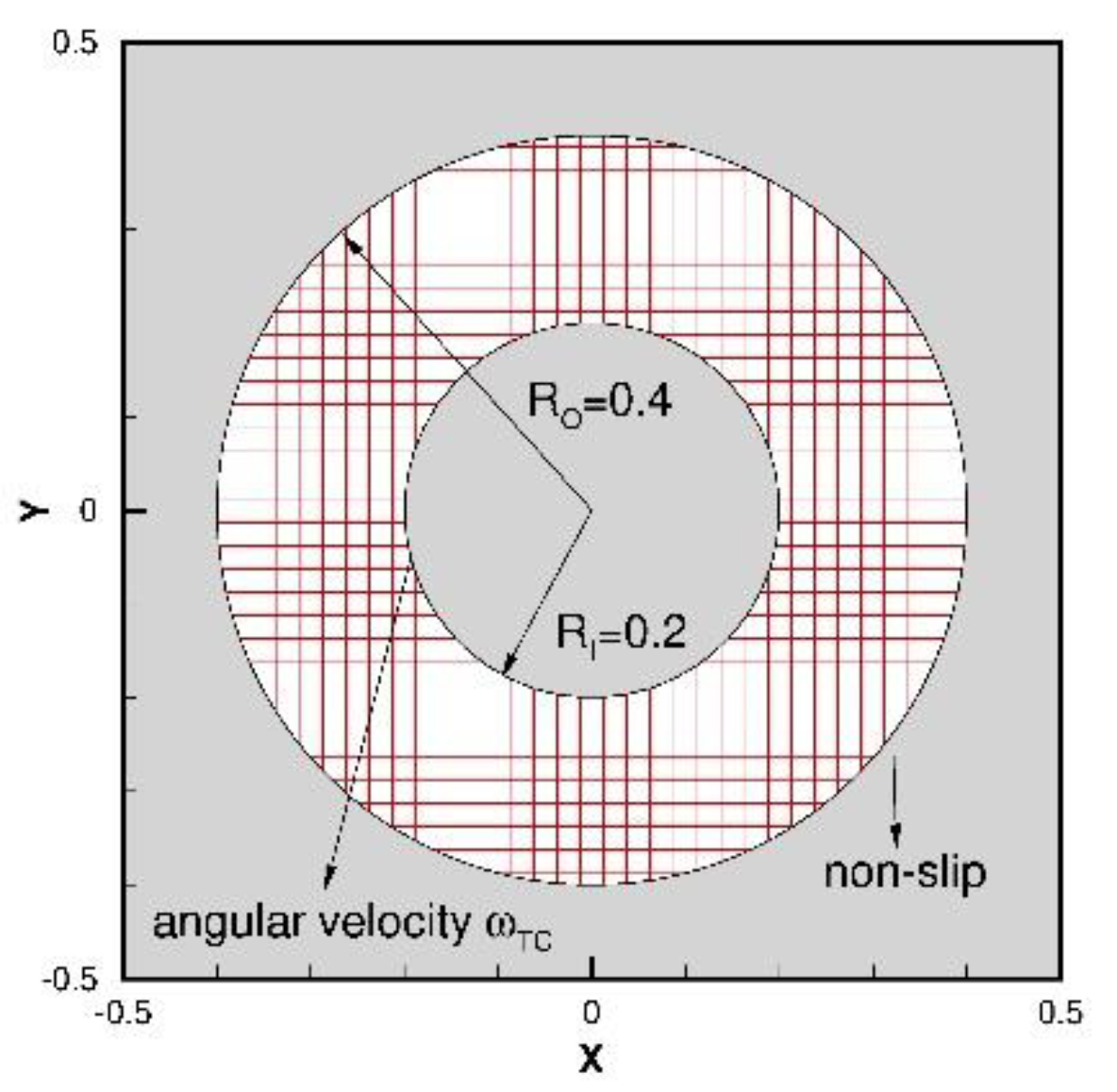
5.1. Taylor-Couette Flow

The 2-D Taylor–Couette flow problem has been chosen as the first validation problem. For the present problem, the radius for outer circular ($R_O)$ and inner circular ($R_I)$ are 0.4 and 0.2. The non-slip boundary condition is employed for the outer circular, and a constant rotating angular velocity ${\omega }_{TC}=3$ is set as a boundary condition for the inner circular. The exact solution for this kind of flow setting can be derived as

$$u\left(x,y\right)=-K\left(\frac{R_O^2}{r^2}-1\right)y$$

(37)

$$v\left(x,y\right)=K\left(\frac{R_O^2}{r^2}-1\right)x$$

(38)

$$p\left(x,y\right)=K^2(\frac{r^2}{2}-\frac{R_O^2}{2r^2}-R_2^2\log \left(r^2\right))$$

(39)

$$K=\frac{{\omega }_{TC}{R}_I^2}{R_O^2-R_I^2}$$

(40)

$$r=\sqrt{x^2-y^2}$$

(41)

For the present study, four different mesh sizes, namely $\mathsf{\Delta }x=\mathsf{\Delta }y=\mathsf{\Delta }h=1/10$, $1/20$, $1/40$ and $1/80$ with $Re=500$ are conducted for the validation study in a unit square domain. The inner and outer cylinder are modeled with DIIB method, as shown in Figure 4.

From

Table 1. The error L-2 norms for the Taylor–Couette flow problem.

	$\mathit{u}$	$\mathit{v}$	$\mathit{p}$
$\mathsf{\Delta }h$ = 1/10	3.380 × 10−2	3.380 × 10−2	2.053 × 10−2
$\mathsf{\Delta }h$ = 1/20	2.214 × 10−2	2.214 × 10−2	9.046 × 10−3
$\mathsf{\Delta }h$ = 1/40	1.911 × 10−3	1.911 × 10−3	9.115 × 10−4
$\mathsf{\Delta }h$ = 1/80	4.928 × 10−4	4.928 × 10−4	2.923 × 10−4

and Figure 5, this shows that the rate of convergence for $u$, $v$ and $p$ are 2.033, 2.033 and 2.044, which match very well with the proposed accuracy order. The validation of the present solver was then confirmed.

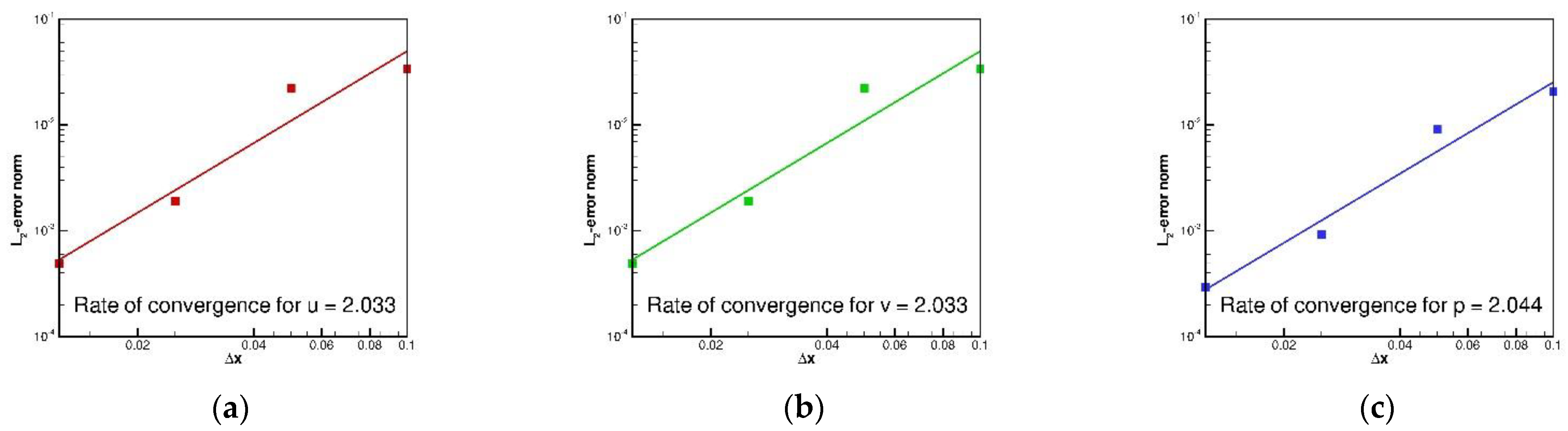
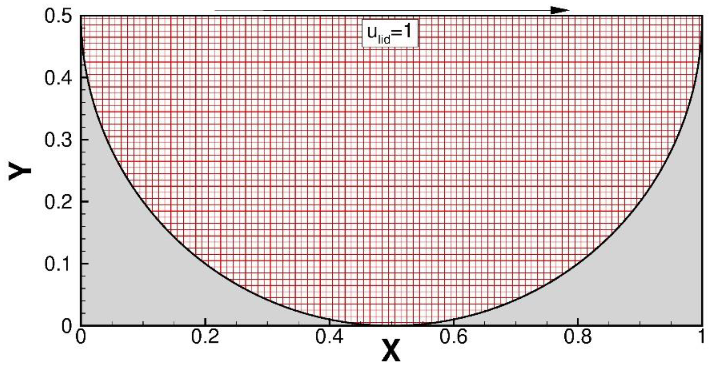
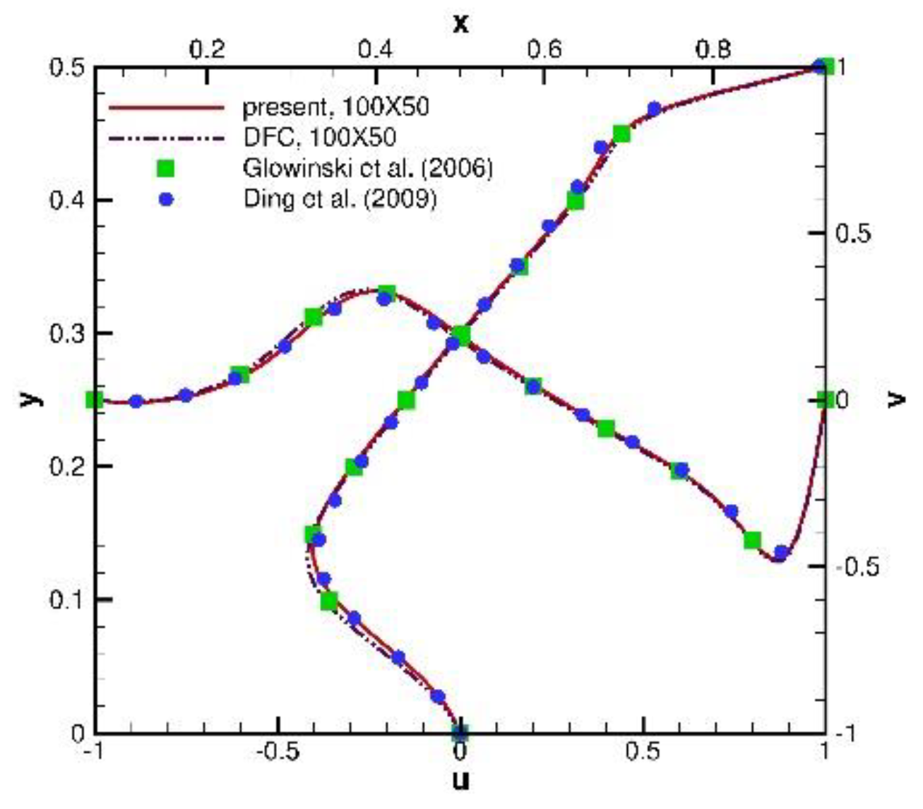
5.2. Lid-Driven Semi-Circular Cavity Flow

To further understand the performance of the present framework, the lid-driven semi-circular cavity flow problem was then investigated. In a 1 × 0.5 rectangular domain, there is a semi-circular cavity with a radius of 0.5 modeled by immersed boundary method, and the lid is driven with velocity $u_{lid}=1$, as shown in Figure 6. Comparisons of cutting-line velocity at $x=0.5$ and $y=0.25$ with the benchmarking solutions of Glowinski et al. [21] and Ding et al. [22] were made with $Re=1000$ and 100 × 50 mesh. This shows excellent agreement with Figure 7. To further show the accuracy of the present IDFC² framework, we also plotted the numerical results which was obtained by the fifth order upwinding scheme-based DFC framework [23]. As can be seen in Figure 7, the present results match better than the reference results. For the sake of completeness, the predicted contours of pressure and vorticity are also plotted in Figure 8 to show the applicability of the present framework.

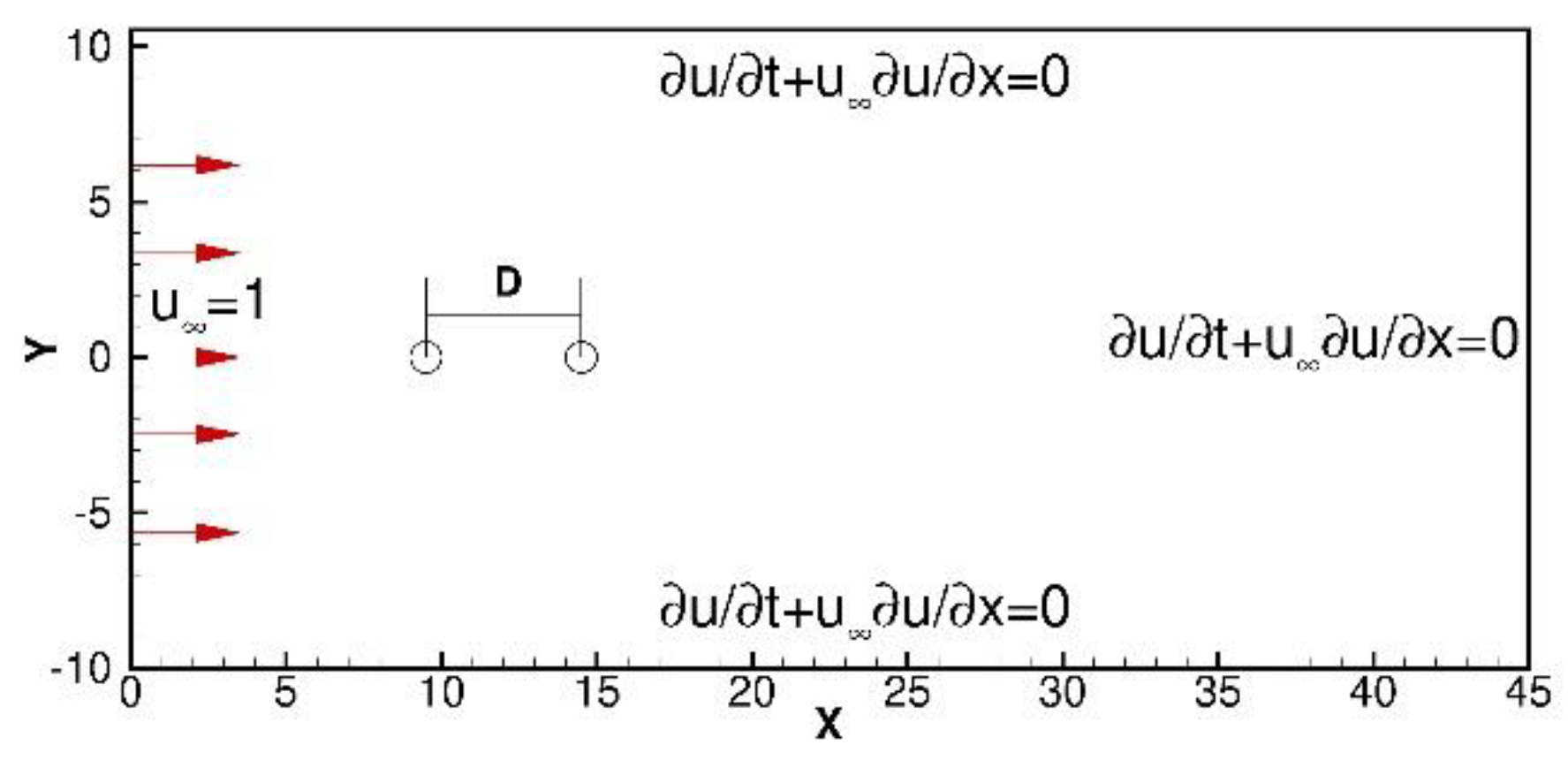
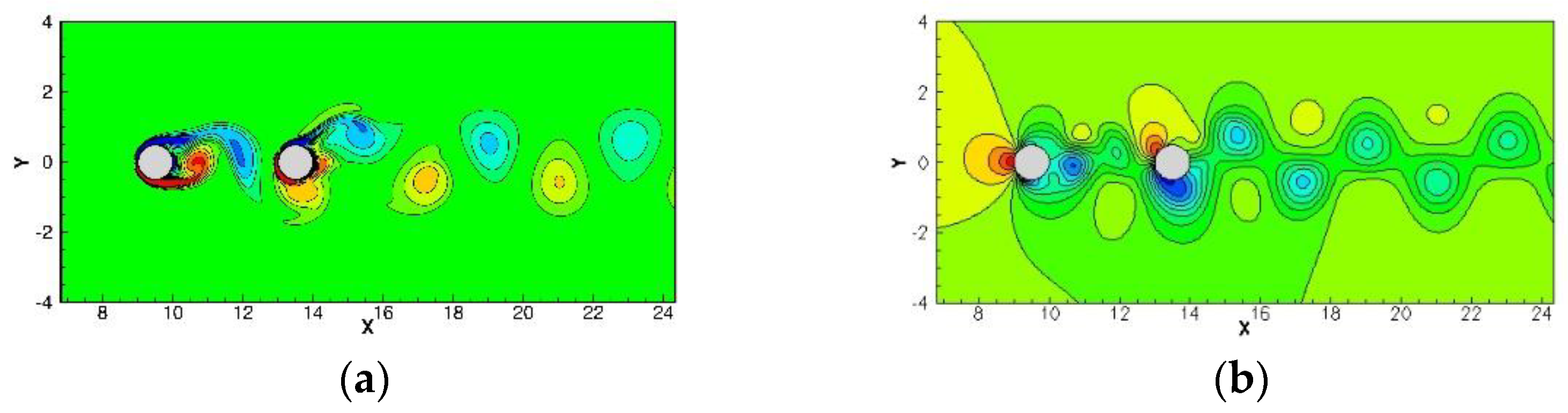
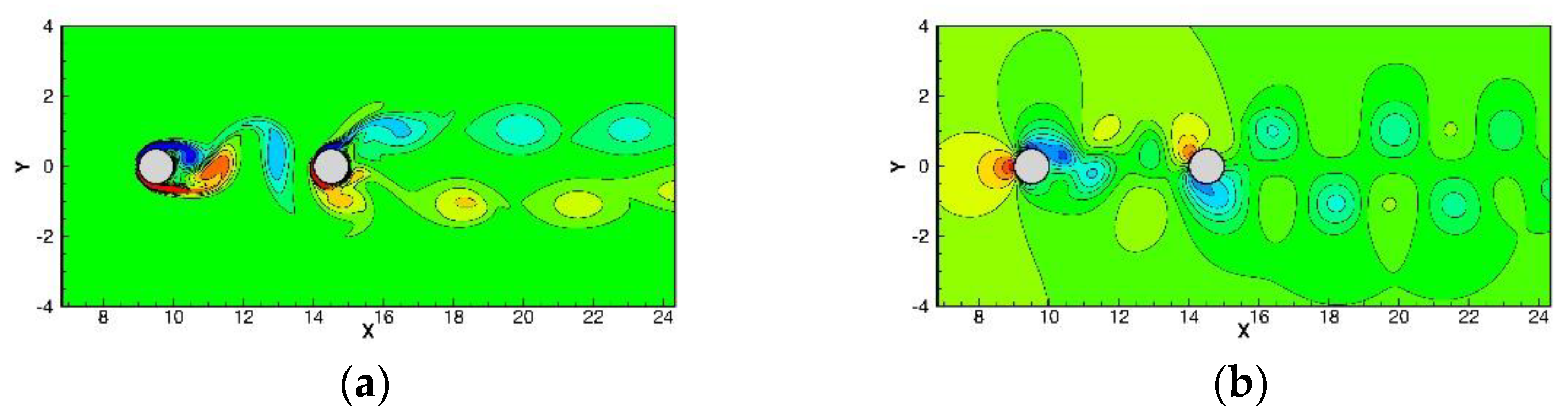
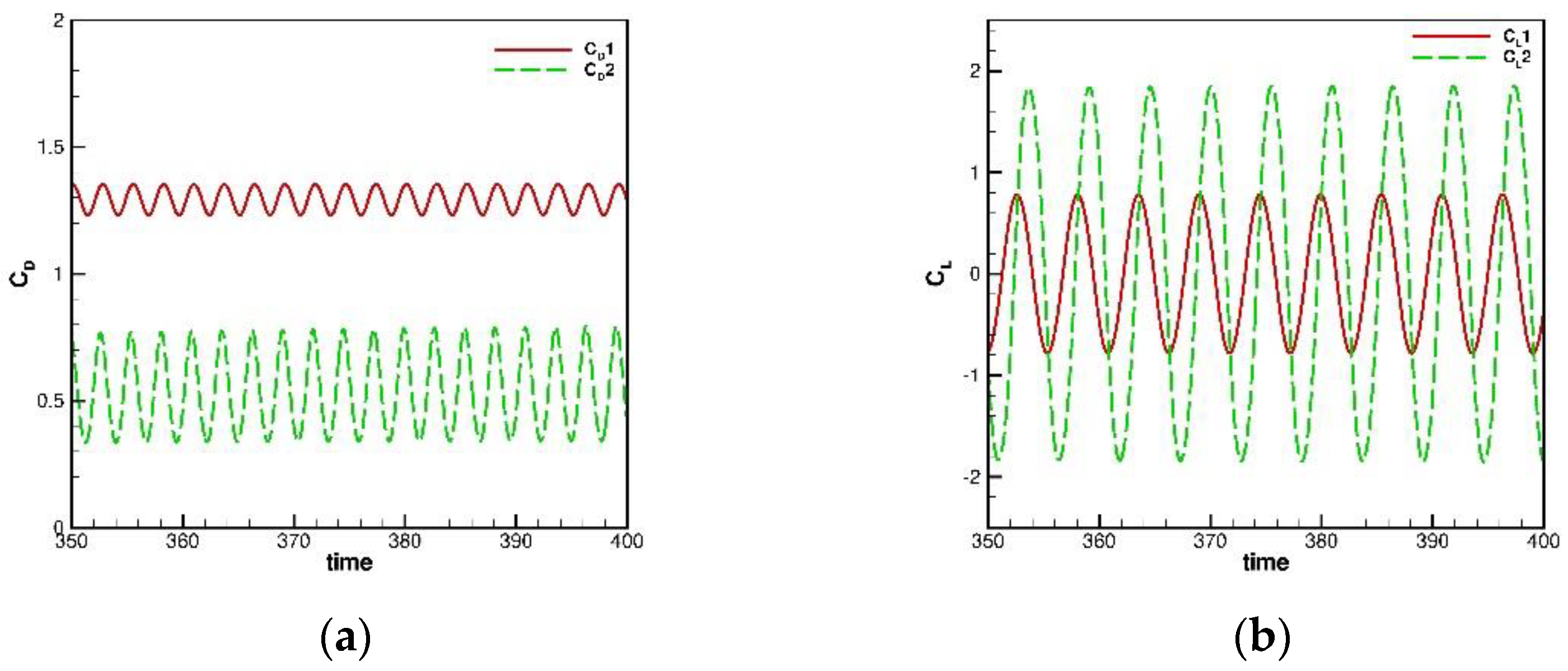
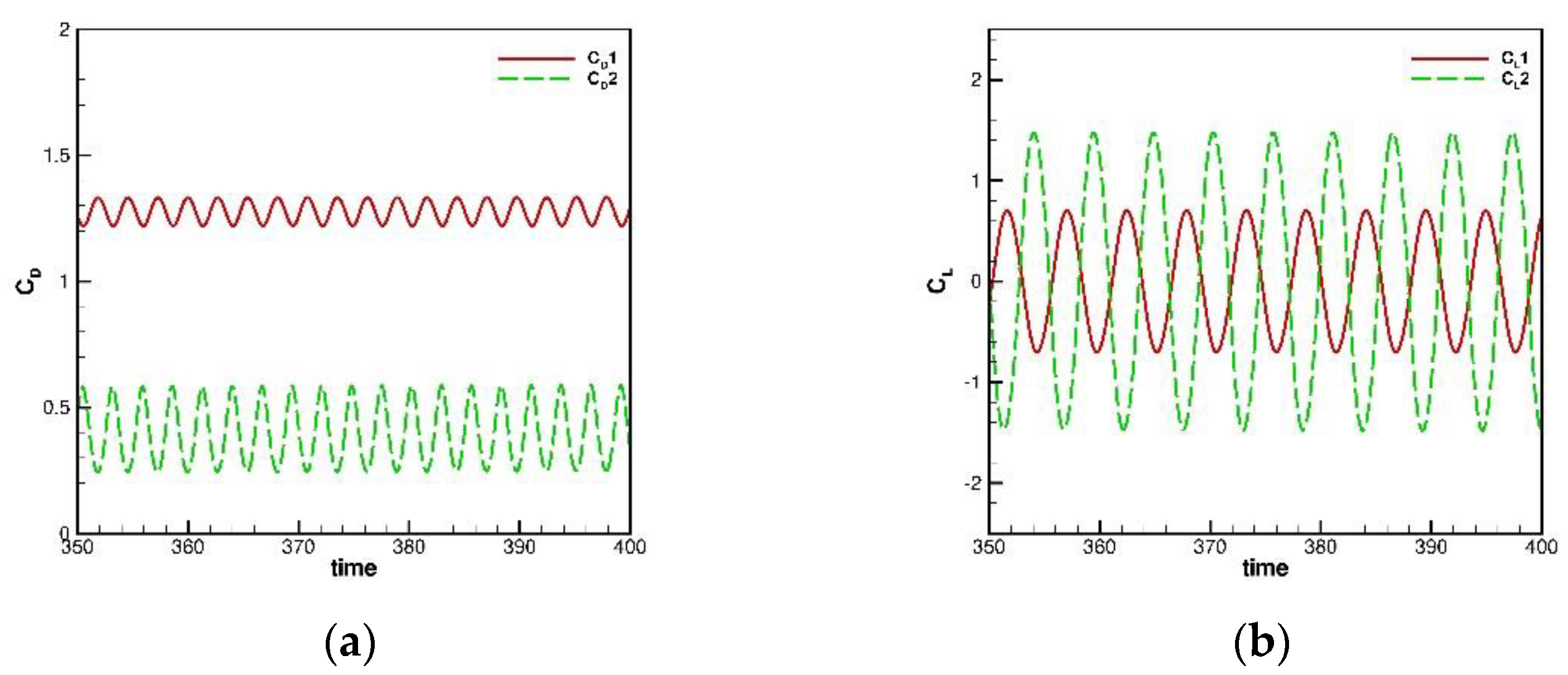
5.3. Flow Past Circular Cylinders in Tandem

In this subsection, the flow past circular cylinders in tandem problem will be simulated to show that the present framework can produce accurate solutions for time transient flows. For this problem the computational domain is set as a 45 × 20 rectangular domain at the inlet with velocity $u_{\infty }=1$ from the left boundary, while the other three boundaries are set as convective boundary conditions. Inside the computational domain, there are two circular cylinders with diameter $d=1$ in tandem. The centroid of the left one is located at (9.5, 0), while the right one is located at (9.5 + D, 0), where D is the distance between two circular centroids. In this study, two scenarios of D = 4 and D = 5 with $Re=200$ and mesh size $\Delta x=\Delta y=d/20$ were investigated. The details of the present settings are plotted in Figure 9. The simulated vorticity and pressure contours at t = 400 are plotted in Figure 10 and Figure 11 for D = 4 and D = 5, respectively. As shown in Figure 10 and Figure 11, the present framework can correctly produce the vortex shedding behavior, while the pressure can remain smooth. The predicted results were then used to evaluate the drag coefficient ($C_D$), lift coefficient ($C_L$) and Strouhal number ($St$), and compare with the referenced solutions ([24,25,26,27]). From

Table 2. Comparisons of $C_D$, $C_L$ and $St$ for the flow past circular cylinders in tandem problem with $Re=200$. Note that $C_{D}1$ is the left circular cylinder, while $C_{D}2$ is the right circular cylinder.

	D = 4
	$C_{D}1$	$C_{D}2$	$C_{L}1$	$C_{L}2$	$St$
Meneghini et al., 2001	1.18	0.38	---	---	0.174
Mahir and Altac, 2008	1.34	0.558	0.805	1.99	0.181
Dehkordi et al., 2011	1.16	0.52	---	---	0.179
Slaouti and Stansby, 1992	1.11	0.88	0.7	1.8	0.190
Present study	1.293	0.568	0.783	1.853	0.183
	D = 5
	$C_{D}1$	$C_{D}2$	$C_{L}1$	$C_{L}2$	$St$
Mahir and Altac, 2008	1.327	0.455	0.731	1.569	0.186
Slaouti and Stansby, 1992	0.97	0.7	0.55	1.6	0.180
Present study	1.277	0.418	0.702	1.482	0.185

, good agreements can be observed between predicted results and benchmarking solutions. The drag and lift coefficient are also plotted in Figure 12 and Figure 13 with respect to time. It is confirmed that the present framework for transient flows is applicable and accurate.

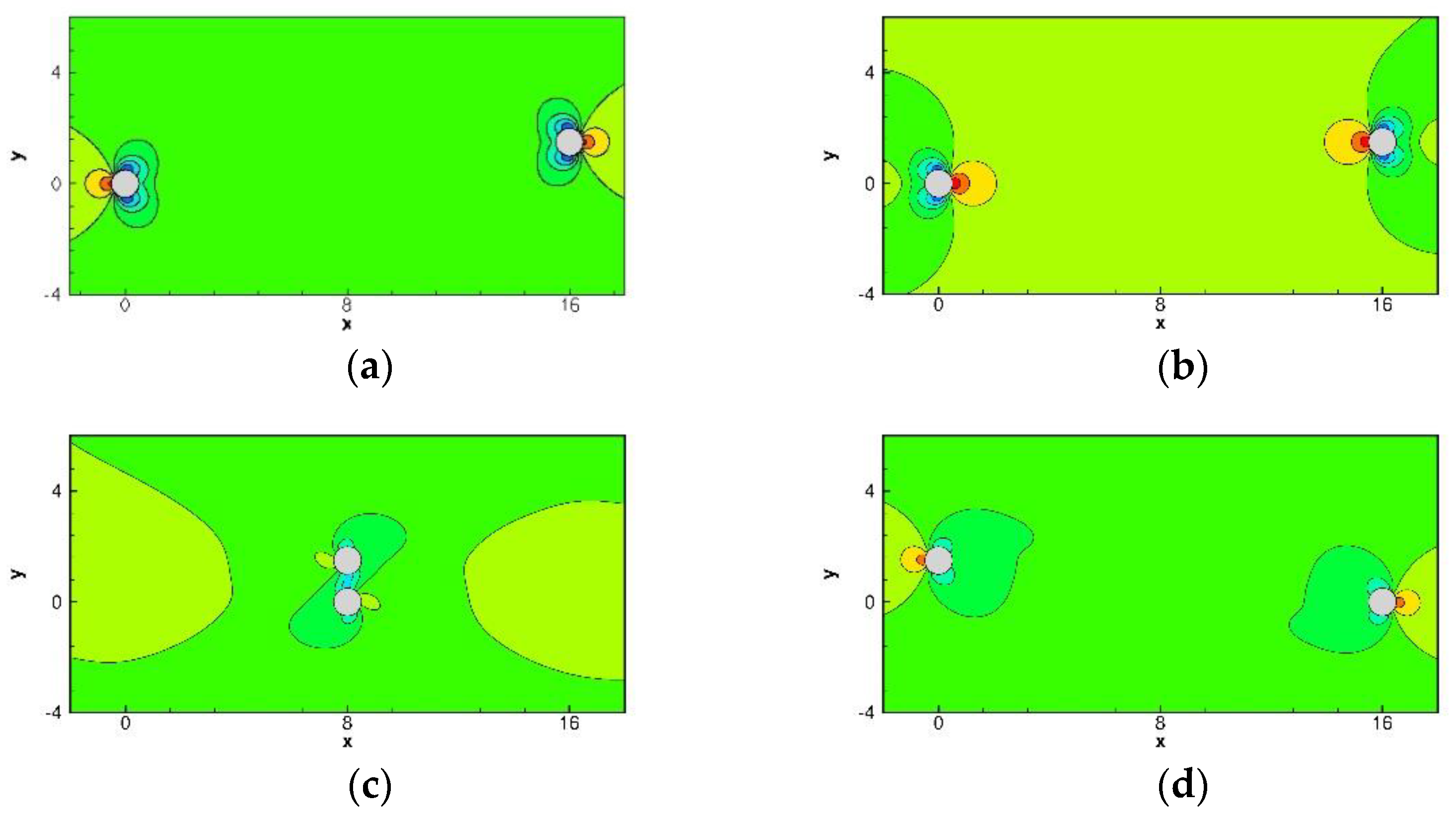
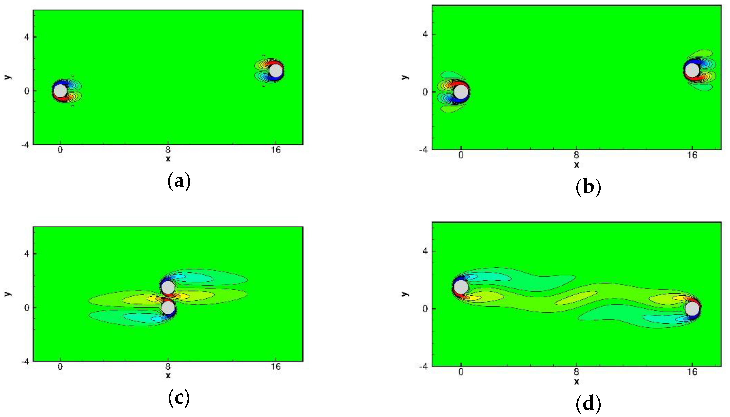
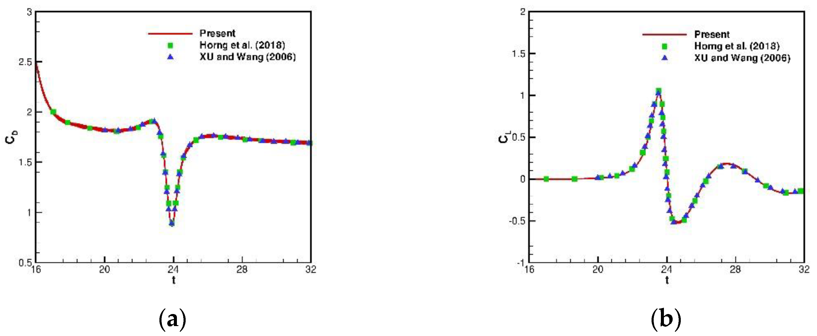
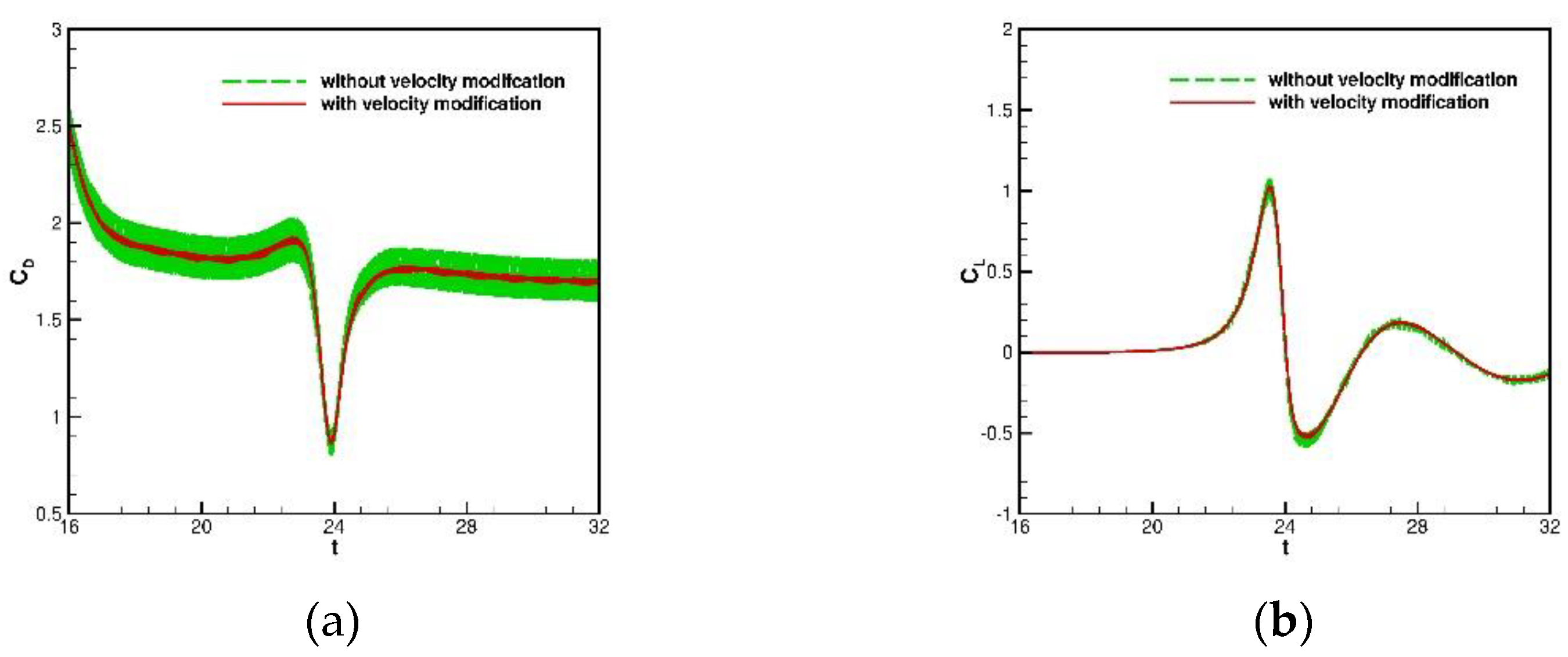
5.4. Two Circular Cylinders Moving towards Each Other in Quiescent Flow

In the computational domain $\left(x=-8~24,y=-8~8\right)$, there are two circular cylinders with a unit diameter (d = 1), the lower initially located at ($x_l,y_l=0,0$), while the upper one located at $\left(x_u,y_u=16,1.5\right)$, and then moving toward each other along the x direction with the prescribed motions until $t$ = 32:

$$x_l\left(t\right)=\{\begin{array}{cc}\frac{4}{\pi }\sin (\frac{\pi t}{4}), & 0\le t\le 16\\ t-16,& 0\le t\le 32\end{array}$$

(42)

$$x_u\left(t\right)=\{\begin{array}{cc}16-\frac{4}{\pi }\sin (\frac{\pi t}{4}), & 0\le t\le 16\\ 32-t,& 0\le t\le 32\end{array}$$

(43)

Based on the above prescribed motions, two cylinders will move periodically in the x axis until $t$ = 16, then start to move towards each other. In this study, a no-slip boundary condition is applied to all boundaries, and the mesh size and time step size are chosen as $\Delta x=\Delta y=d/40$ and $\Delta t={10}^{-2}$. From Figure 14 and Figure 15, it shows that the present framework can produce smooth pressure and vorticity. To validate the accuracy of the predicted results, we plotted Figure 16 to compare the time-history drag (C_D) and lift (C_L) coefficients of the upper cylinder with the referenced solutions [9,28] which shows excellent agreements. For the sake of completeness, we also plotted Figure 17 to show the effect of velocity modification method. This clearly shows that with the velocity modification method, SFO is well suppressed.

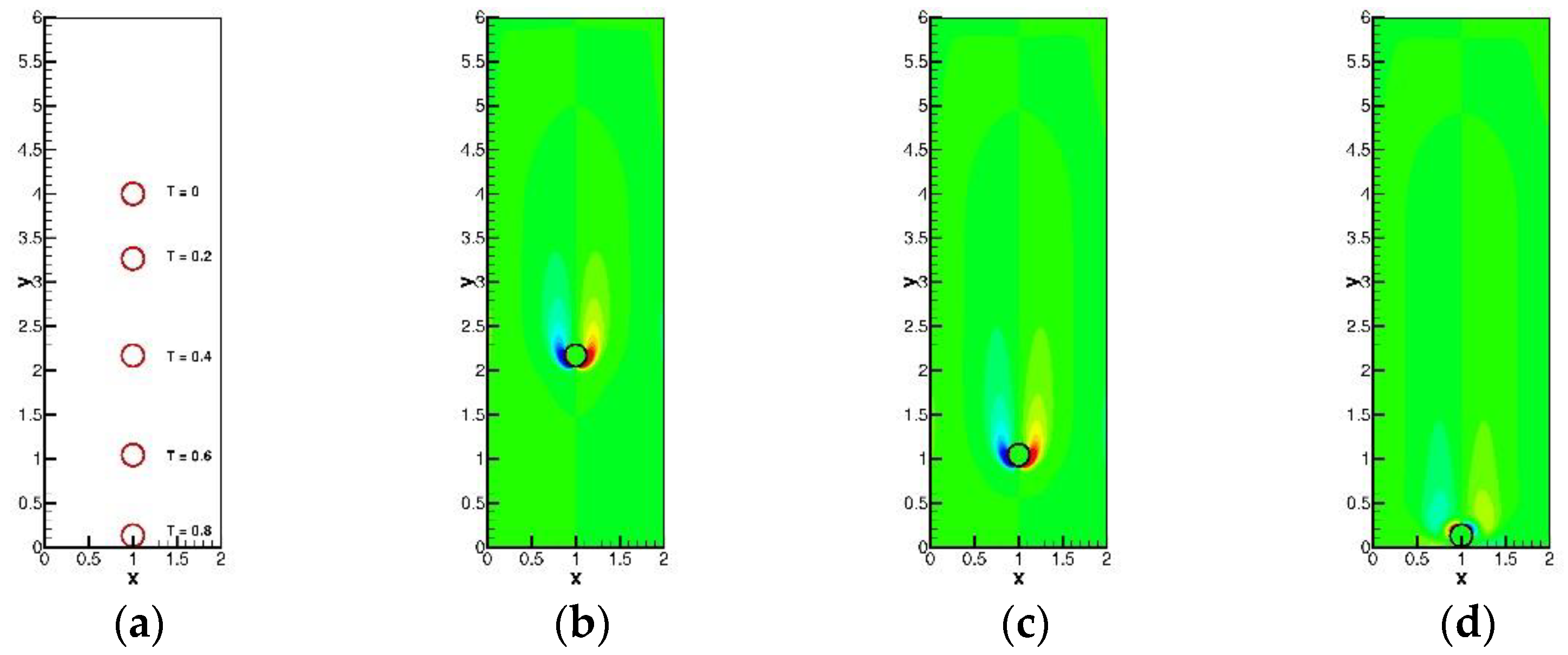
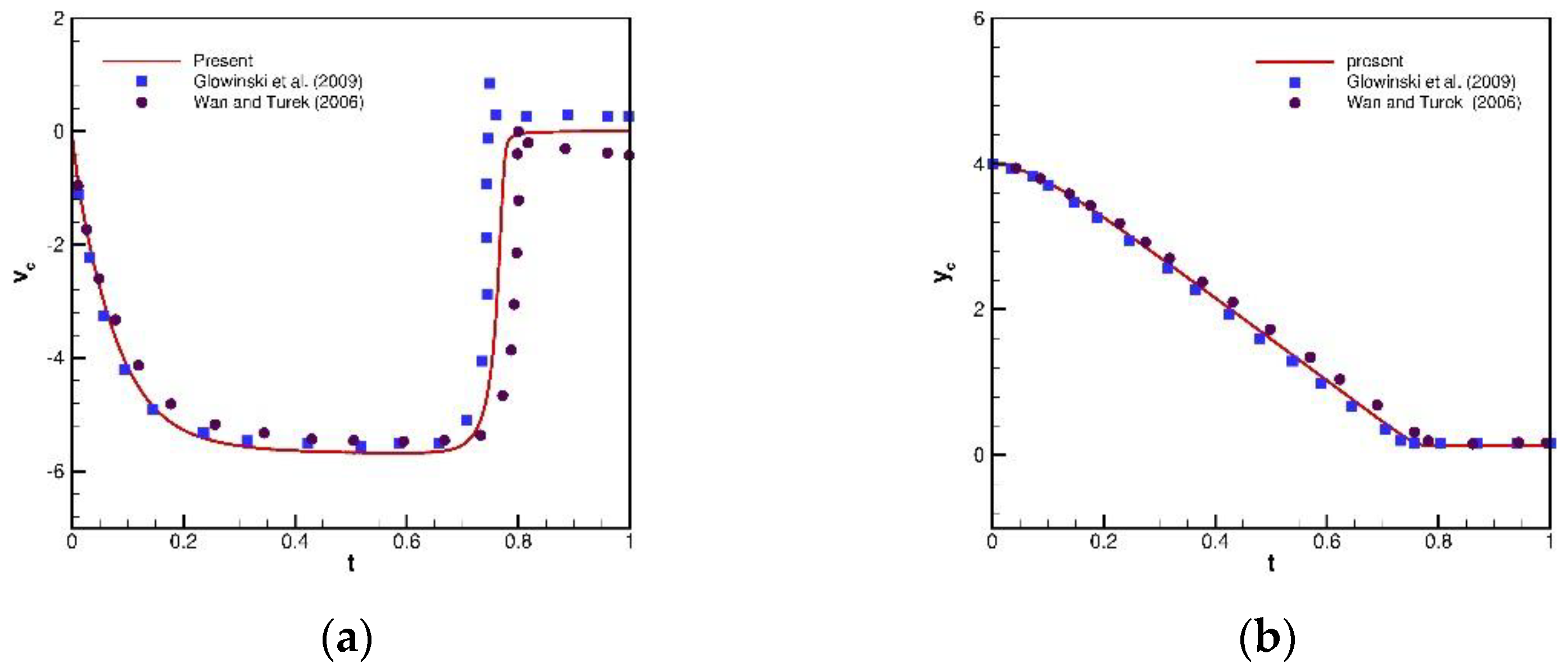
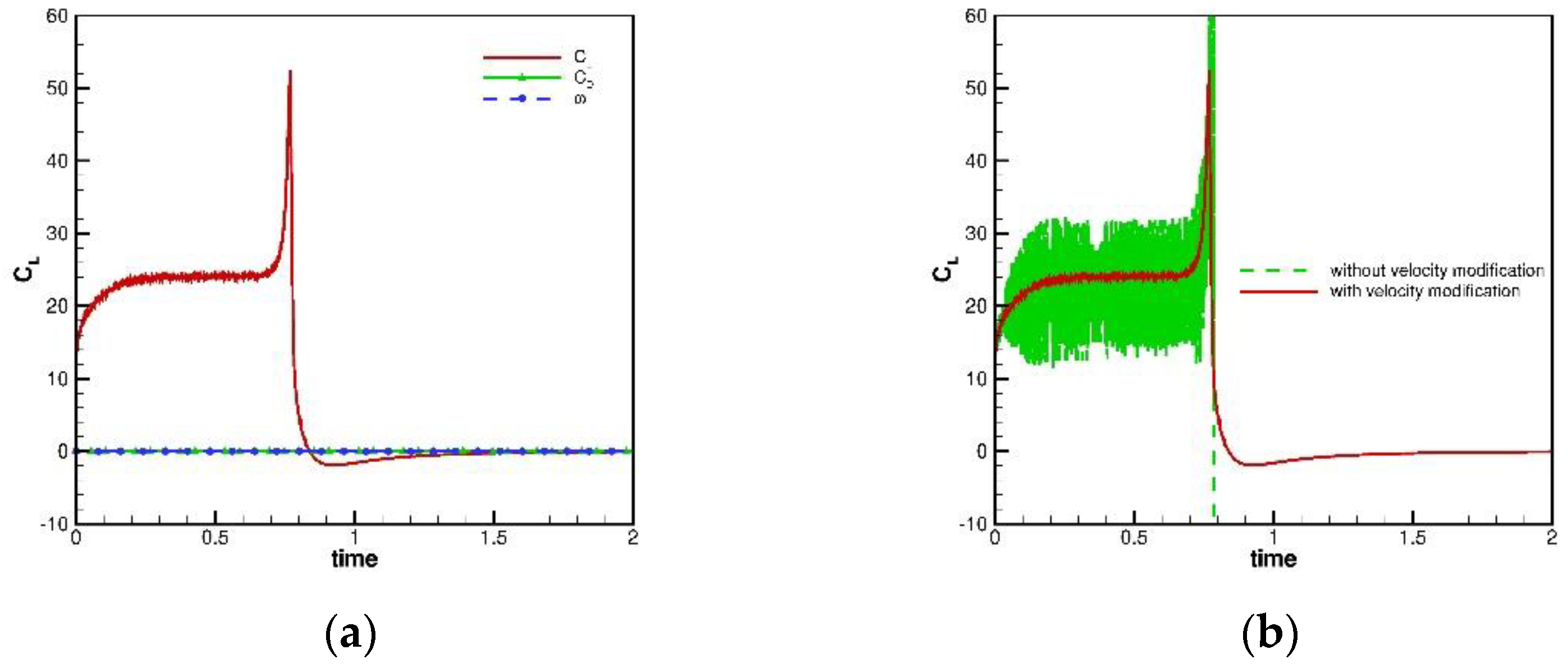
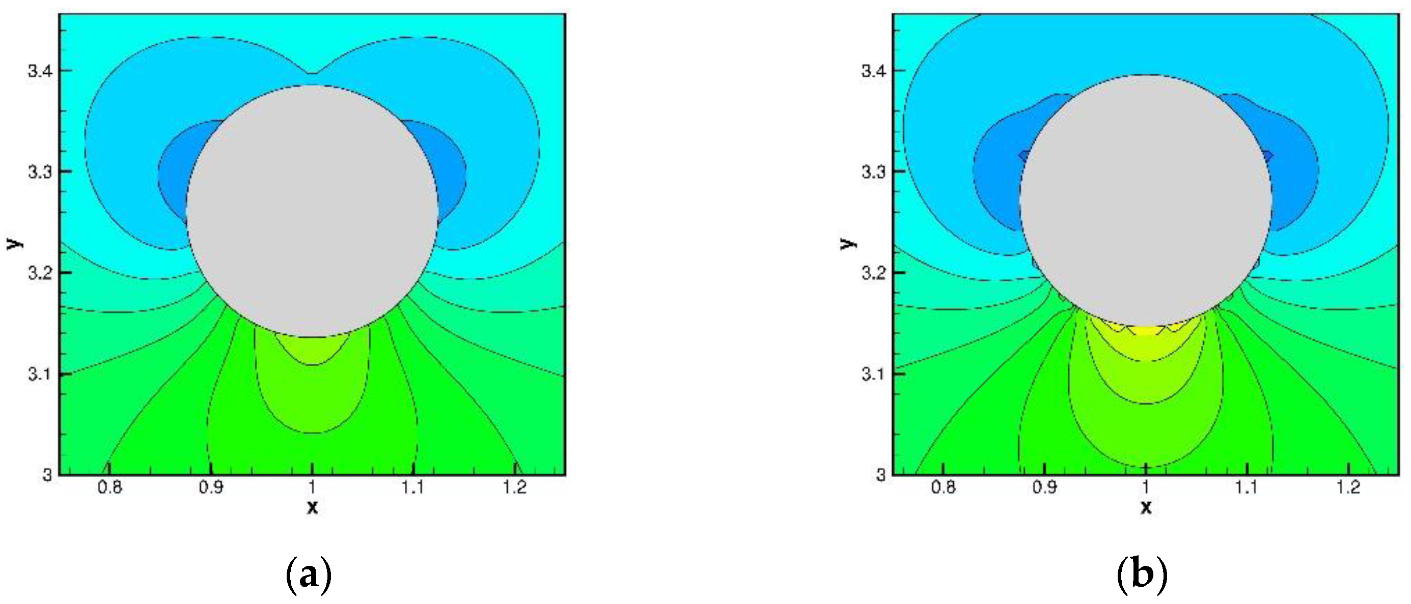
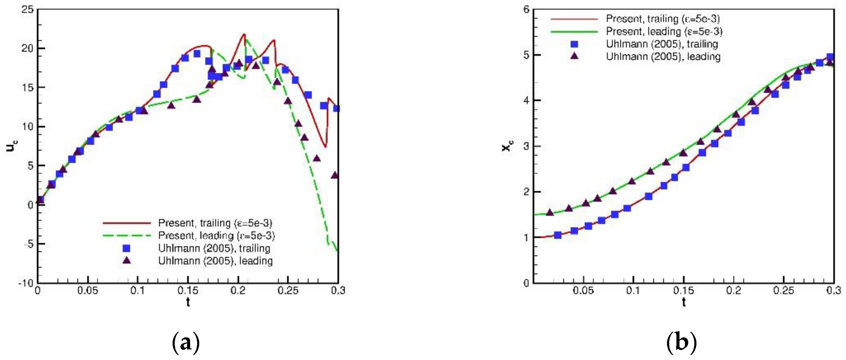
5.5. Free-Falling Circular Cylinder in Quiescent Flow

The free-falling circular cylinder problem will be simulated in this subsection. In a 2 × 6 rectangular box, a circular cylinder located at (1,4) with a radius r = 0.125 is free falling from rest, as shown in Figure 18a. The densities of solid $\left({\rho }_s\right)$ and fluid $\left({\rho }_f\right)$ are 1.25 and 1, while the non-dimensional fluid viscosity and gravity for the investigated problem are 0.1 and (0, −980). The cylinder positions and vorticity contours at different times are plotted in Figure 18. In order to validate the present framework, comparisons of the time history of cylinder positions and velocity are also plotted at Figure 19. It can be clearly shown that the preset results obtained by the proposed framework and methodology with $\Delta x=\Delta y=1/128$ and $\Delta t={10}^{-4}$ agree well with the reference benchmark results [29,30]. For the sake of completeness, C_D, C_L and $\omega$ are plotted in Figure 20a, while the effect of velocity modification method is plotted in Figure 20b. From Figure 20, it shows that the present framework can also well suppress for the free-falling cylinder problem. The pressure contours at t = 0.2 are also plotted to further show the benefit of employing velocity modification method. From Figure 21a, the smooth pressure is obtained, while Figure 21b clearly shows oscillated pressure near the downward cylinder interface.

To show the advantage of the present framework, different density ratios (${\rho }_s/{\rho }_f$), 1.05 and 1.01, were also investigated in this study. Figure 22 clearly shows that the present framework can correctly and consistently predict solid velocity and position. The applicability and efficiency of the present framework for solving the free-falling cylinder problem is thus confirmed.

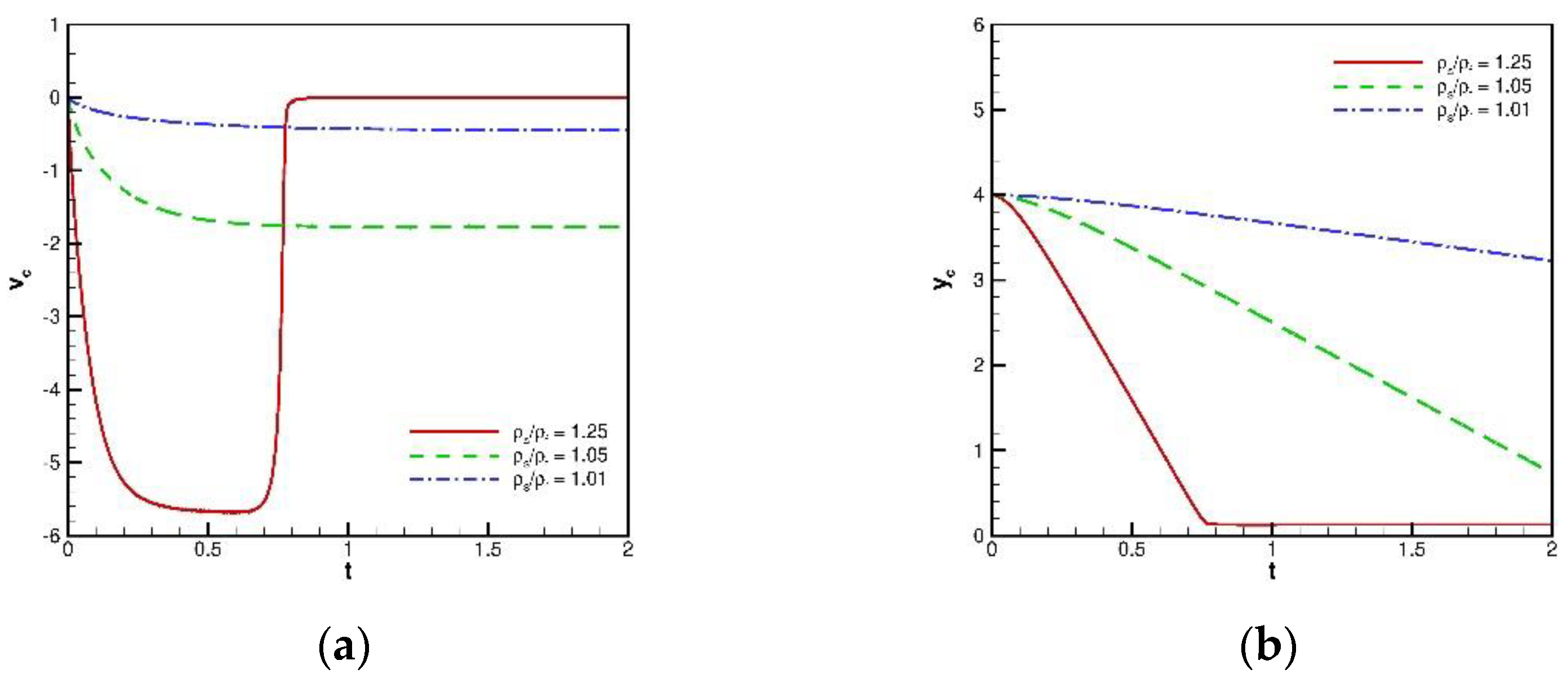
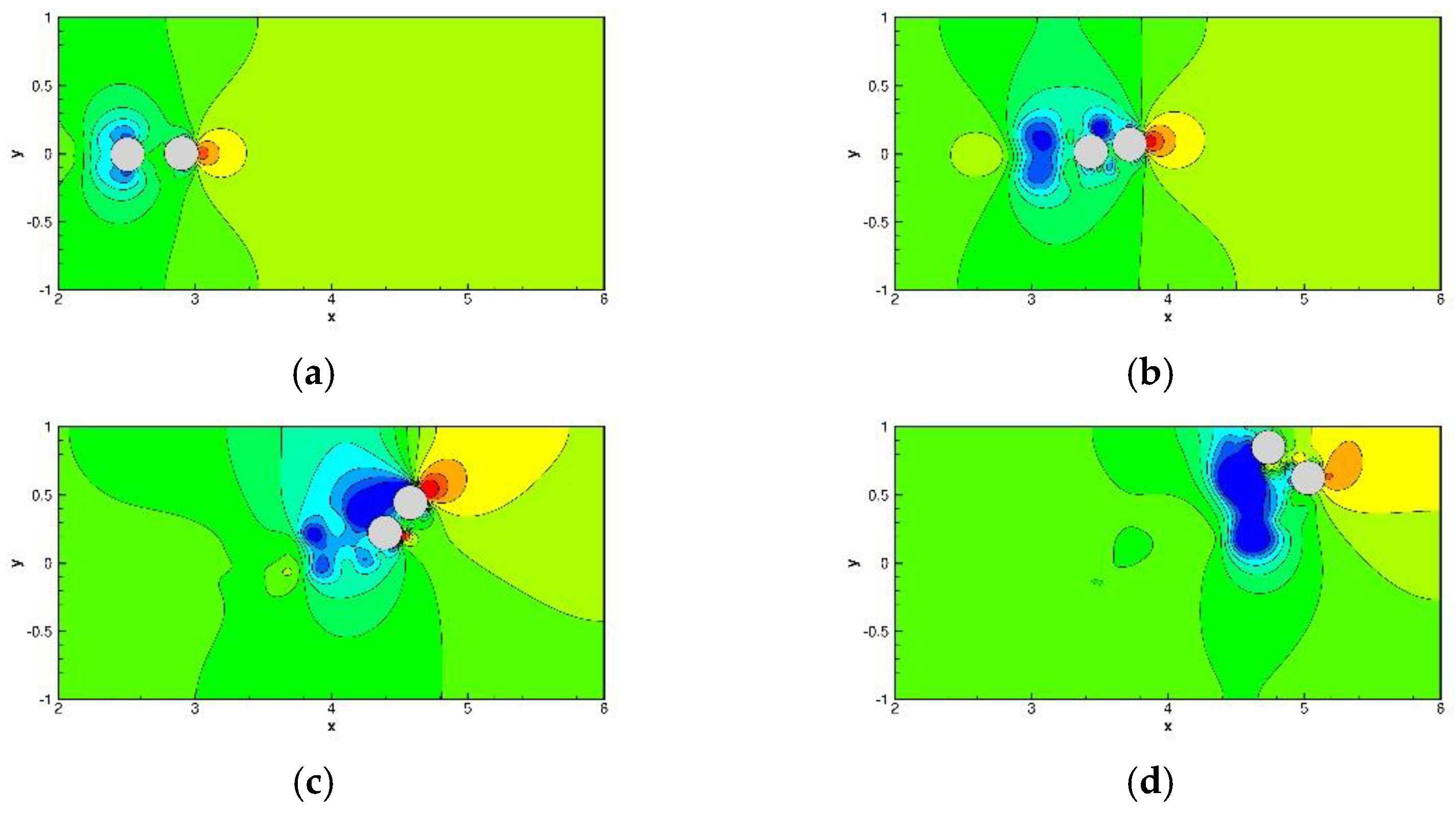
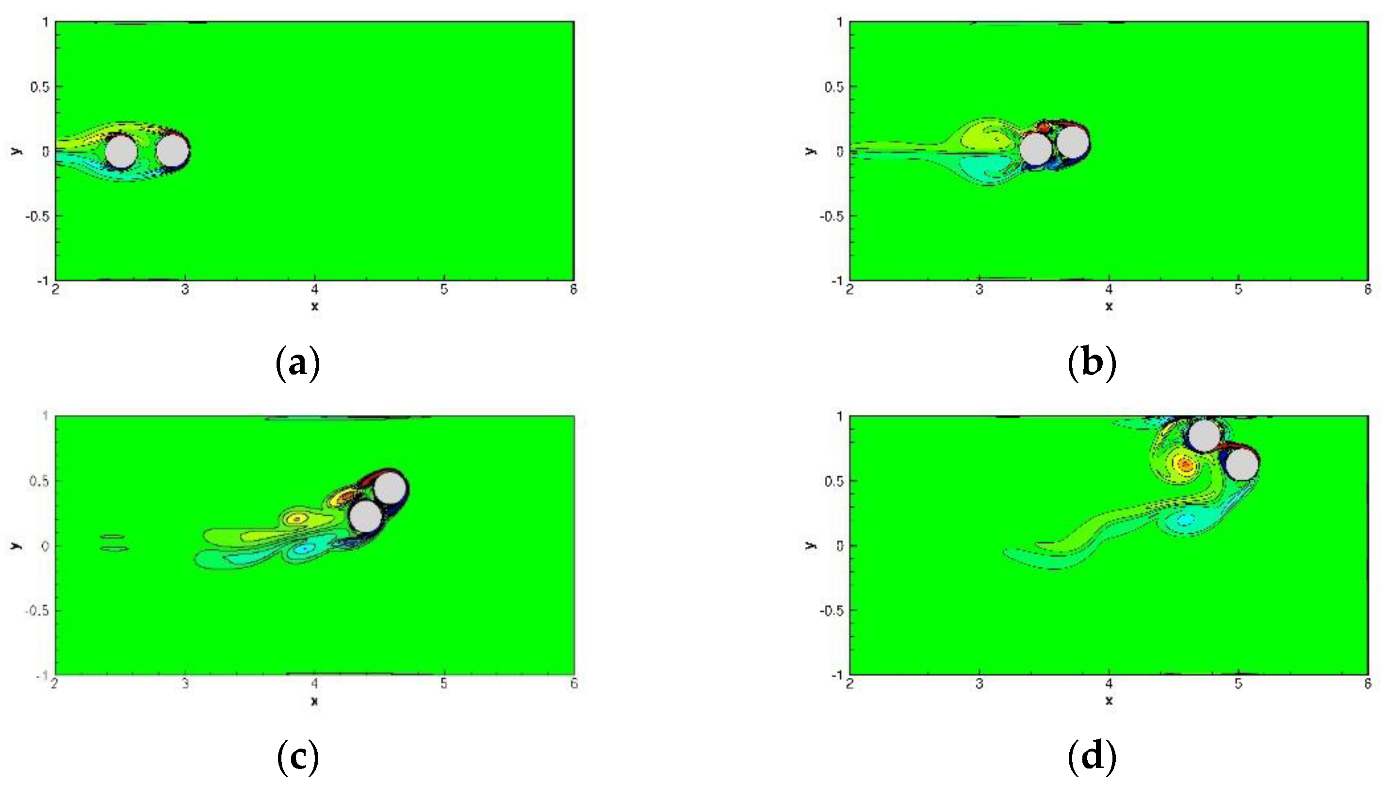
5.6. Drafting–Kissing–Tumbling (DKT) Problem of Two Free-Falling Circular Cylinders in Quiescent Flow

Finally, the drafting–kissing–tumbling (DKT) problem was investigated in this subsection. In a computational domain of $\left(x,y\right)=\left(0~6,-1~1\right)$, there are two cylinders with a radius r = 0.125 located at (1, 0.001) and (1.5, −0.001). The density ratio and viscosity ratio was chosen as 1.5 and 0.01, while the gravity is (980, 0). To model the DKT scenario in this study, the repulsion force model [29] was employed in this study, with the choice of a stiffness parameter as $5\times {10}^{-3}$ and effective force range as $3\mathsf{\Delta }x$. Due to the large repulsion force, the sub-time stepping method is employed to prevent the divergence issue when solving the equations of motions. The idea is to introduce a sub-time step $\mathsf{\Delta }{t}_s\left(=\mathsf{\Delta }t/s\right)$, which is $s$ times smaller than the original time step $\mathsf{\Delta }t$, and solves the sub-time step $s$ times. In practice, the fluid solver costs the most of the computational time, so the additional cost due to the sub-time stepping can be ignored. In this study, the sub-time step $s$ is set as 20. The predicted pressure and vorticity contours with $\mathsf{\Delta }x=\mathsf{\Delta }y=1/256$ and $\mathsf{\Delta }t=5\times {10}^{-5}$ at t = 0.15, 0.2, 0.25 and 0.3 are plotted in Figure 23 and Figure 24. The comparisons of solid velocity and position with the referenced solution [2] are then made. From Figure 25 and Figure 26, good agreements can be seen at $t\le 0.17$, (drafting and first kissing stage). For $t>0.17$ (the later kissing and tumbling stage), it still shows reasonable agreements. As indicated by [2], the discrepancy should be due to strong instability and the choice of collision parameter and the initial horizontal offset of two cylinders. It is noted that there is no drafting for the present framework if the horizontal offset is set to zero.

6. Conclusions

In this study, we proposed a framework to model the flow–particle interaction problem. The solid object is modeled by the DIIB method, while the fluid velocity and pressure are solved by the IDFC² method. To prevent the instability problem of a density ratio close to 1, the hydrodynamic force and torque which appeared in the equations of motion are directly evaluated with modified interpolation kernel function. The methodology of evaluating the drag/lift forces and the treatment of a circular cylinder approaching the wall have also been addressed. To validate the applicability and accuracy, problems of one and two particles were investigated. To make the framework more stable, the idea of a sub-time stepping method was also employed for DKT problems of two particles. From the investigating validation/benchmarking problems, the simulated results reveal the applicability, accuracy and efficiency of the present framework.

References

1. Peskin, C.S. The immersed boundary method. Acta Numer. 2002, 11, 479–517. [Google Scholar] [CrossRef] [Green Version]
2. Uhlmann, M. An immersed boundary method with direct forcing for the simulation of particulate flows. J. Comput. Phys. 2005, 209, 448–476. [Google Scholar] [CrossRef] [Green Version]
3. Kempe, T.; Fröhlich, J. An improved immersed boundary method with direct forcing for the simulation of particle laden flows. J. Comput. Phys. 2012, 231, 3663–3684. [Google Scholar] [CrossRef]
4. Breugem, W.P.A. Second-order accurate immersed boundary method for fully resolved simulations of particle-laden flows. J. Comput. Phys. 2012, 231, 4469–4498. [Google Scholar] [CrossRef]
5. Zhang, L.T.; Gay, M. Immersed finite element method for fluid-structure interactions. J. Fluid Struct. 2007, 23, 839–857. [Google Scholar] [CrossRef]
6. Luo, K.; Wang, Z.; Fan, J. A modified immersed boundary method for simulations of fluid–particle interactions. Comput. Methods Appl. Mech. Eng. 2007, 197, 36–46. [Google Scholar] [CrossRef]
7. Wang, Z.; Fan, J.; Luo, K. Combined multi-direct forcing and immersed boundary method for simulating flows with moving particles. Int. J. Multiph. Flow 2008, 34, 283–302. [Google Scholar] [CrossRef]
8. Yang, J.; Stern, F. A Sharp Interface Direct Forcing Immersed Boundary Approach for Fully Resolved Simulations of Particulate Flows. J. Fluids Eng. 2014, 136, 040904. [Google Scholar] [CrossRef]
9. Horng, T.L.; Hsieh, P.W.; Yang, S.Y.; You, C.S. A simple direct-forcing immersed boundary projection method with prediction-correction for fluid-solid interaction problems. Comput. Fluids 2018, 176, 135–152. [Google Scholar] [CrossRef]
10. Wu, J.; Shu, C. Particulate Flow Simulation via a Boundary Condition-Enforced Immersed Boundary-Lattice-Boltzmann Scheme. Commun. Comput. Phys. 2010, 7, 793–812. [Google Scholar]
11. Hao, J.; Zhu, L. A lattice Boltzmann based implicit immersed boundary method for fluid–structure interaction. Comput. Math. Appl. 2010, 59, 185–193. [Google Scholar] [CrossRef] [Green Version]
12. Wang, L.; Guo, Z.; Shi, B.; Zheng, C. Evaluation of Three Lattice Boltzmann Models for Particulate Flows. Commun. Comput. Phys. 2013, 13, 1151–1172. [Google Scholar] [CrossRef]
13. Zhou, Q.; Fan, L.S. A second-order accurate immersed boundary-lattice Boltzmann method for particle-laden flows. J. Comput. Phys. 2014, 268, 269–301. [Google Scholar] [CrossRef]
14. Zhang, H.; Trias, F.S.; Oliva, A.; Yang, D.; Tan, Y.; Shu, S.; Sheng, Y. PIBM: Particulate immersed boundary method for fluid–particle interaction problems. Powder Technol. 2015, 272, 1–13. [Google Scholar] [CrossRef] [Green Version]
15. Coclite, A.; Ranaldo, S.; de Tullio, M.D.; Decuzzi, P.; Pascazio, G. Kinematic and dynamic forcing strategies for predicting the transport of inertial capsules via a combined lattice Boltzmann-Immersed Boundary method. Comput. Fluids 2019, 180, 41–53. [Google Scholar] [CrossRef] [Green Version]
16. Coclite, A.; Ranaldo, S.; Pascazio, G.; Tullio, M.D. de A Lattice Boltzmann dynamic-Immersed Boundary scheme for the transport of deformable inertial capsules in low-Re flows. Comput. Math. Appl. 2020, 80, 2860–2876. [Google Scholar] [CrossRef]
17. Chiu, P.H.; Poh, H.J. Development of an improved divergence-free-condition compensated coupled framework to solve flow problems with time-varying geometries. Int. J. Numer. Meth. Fluids 2021, 93, 44–70. [Google Scholar] [CrossRef]
18. Chiu, P.H.; Lin, R.K.; Sheu, T.W.H. A differentially interpolated direct forcing immersed boundary method for predicting incompressible Navier–Stokes equations in time-varying complex geometries. J. Comput. Phys. 2010, 229, 4476–4500. [Google Scholar] [CrossRef]
19. Yang, X.L.; Zhang, X.; Li, Z.L.; He, G.W. A smoothing technique for discrete delta functions with application to immersed boundary method in moving boundary simulations. J. Comput. Phys. 2009, 228, 7821–7836. [Google Scholar] [CrossRef]
20. Chiu, P.H. An improved divergence-free-condition compensated method for solving incompressible flows on collocated grids. Comput. Fluids 2018, 162, 39–54. [Google Scholar] [CrossRef]
21. Glowinski, R.; Guidoboni, G.; Pan, T.W. Wall-driven incompressible viscous flow in a two-dimensional semi-circular cavity. J. Comput. Phys. 2006, 216, 79–91. [Google Scholar] [CrossRef]
22. Ding, L.; Shi, W.; Luo, H.; Zheng, H. Investigation of incompressible flow within 1/2 circular cavity using lattice Boltzmann method. Int. J. Numer. Meth. Fluids 2009, 60, 919–936. [Google Scholar] [CrossRef]
23. Sheu, T.W.H.; Chiu, P.H. A divergence-free-condition compensated method for incompressible Navier-Stokes equations. Comput. Methods Appl. Mech. Eng. 2007, 196, 4479–4494. [Google Scholar] [CrossRef]
24. Meneghini, J.R.; Saltara, F.; Siqueira, C.L.R.; Ferrari, J.A. Numerical simulation of flow interference between two circular cylinders in tandem and side-by-side arrangements. J. Fluids Struct. 2001, 15, 327–350. [Google Scholar] [CrossRef]
25. Mahir, N.; Altac, Z. Numerical investigation of convective heat transfer in unsteady flow past two cylinders in tandem arrangements. Int. J. Heat Fluid Flow 2008, 29, 1309–1318. [Google Scholar] [CrossRef]
26. Dehkordi, B.G.; Moghaddam, H.S.; Jafari, H.H. Numerical simulation of flow over two circular cylinders in tandem arrangement. J. Hydrodyn. Ser. B 2011, 23, 114–126. [Google Scholar] [CrossRef]
27. Slaouti, A.; Stansby, P.K. Flow around two circular cylinders by the random vortex method. J. Fluids Struct. 1992, 6, 641–670. [Google Scholar] [CrossRef]
28. Xu, S.; Wang, Z.J. An immersed interface method for simulating the interaction of a fluid with moving boundaries. J. Comput. Phys. 2006, 216, 454–493. [Google Scholar] [CrossRef]
29. Glowinski, R.; Pan, T.W.; Hesla, T.I.; Joseph, D.D.; Périaux, J. A fictitious domain approach to the direct numerical simulation of incompressible viscous flow past moving rigid bodies: Application to particulate flow. J. Comput. Phys. 2009, 169, 363–426. [Google Scholar] [CrossRef] [Green Version]
30. Wan, D.; Turek, S. Direct numerical simulation of particulate flow via multigrid FEM techniques and the fictitious boundary method. Int. J. Numer. Meth. Fluids 2006, 51, 531–566. [Google Scholar] [CrossRef] [Green Version]
Figure 1. Schematic of the direct forcing immersed boundary (DIIB) method: (a) evaluation of u S ; and (b) evaluation of u f .
Energies 14 01675 g001
Figure 2. Schematic of the present framework.
Energies 14 01675 g002
Figure 3. Overall algorithm for the present framework.
Energies 14 01675 g003
Figure 4. Schematic of the Taylor–Couette flow problem.
Energies 14 01675 g004
Figure 5. The rate of convergence plot for the Taylor–Couette flow problem. (a) u ; (b) v ; and (c) p .
Energies 14 01675 g005
Figure 6. Schematic of the lid-driven semi-circular cavity flow problem.
Energies 14 01675 g006
Figure 7. Comparisons of the velocity with the referenced solutions at the cutting lines for the lid-driven semi-circular cavity flow problem.
Energies 14 01675 g007
Figure 8. The contour plots for the lid-driven semi-circular cavity flow problem: (a) pressure; and (b) vorticity.
Energies 14 01675 g008
Figure 9. Schematic of the flow past circular cylinders in tandem problem.
Energies 14 01675 g009
Figure 10. The instantaneous contour plots for the flow past circular cylinders in tandem problem, D = 4: (a) vorticity; and (b) pressure.
Energies 14 01675 g010
Figure 11. The instantaneous contour plots for the flow past circular cylinders in tandem problem, D = 5: (a) vorticity; (b) pressure.
Energies 14 01675 g011
Figure 12. The time history plots for the flow past circular cylinders in tandem problem, D = 4. Note that C D 1 is the left circular cylinder, while C D 2 is the right circular cylinder: (a) C D ; and (b) C L .
Energies 14 01675 g012
Figure 13. The time history plots for the flow past circular cylinders in tandem problem, D = 5. Note that C D 1 is the left circular cylinder, while C D 2 is the right circular cylinder: (a) C D ; and (b) C L .
Energies 14 01675 g013
Figure 14. The predicted pressure contour plots for the problem of two cylinders moving towards each other: (a) t = 4; (b) t = 16; (c) t = 24; and (d) t = 32.
Energies 14 01675 g014
Figure 15. The predicted vorticity contour plots for the problem of two cylinders moving towards each other problem. (a) t = 4; (b) t = 16; (c) t = 24; and (d) t = 32.
Energies 14 01675 g015
Figure 16. Comparisons of the time history plots of the upper cylinder for the problem of two cylinders moving towards each other: (a) C D ; and (b) C L .
Energies 14 01675 g016
Figure 17. Comparisons of the effect of the velocity modification method for the problem of two cylinders moving towards each other: (a) C D ; and (b) C L .
Energies 14 01675 g017
Figure 18. The predicted results for the free-falling circular cylinder problem: (a) the cylinder positions at different times; (b) vorticity contours at t = 0.4; (c) vorticity contours at t = 0.6; and (d) vorticity contours at t = 0.8.
Energies 14 01675 g018
Figure 19. Comparisons of the results for the free-falling circular cylinder problem with benchmark results [29,30]: (a) velocity; and (b) centric y location.
Energies 14 01675 g019
Figure 20. The time history plots for the free-falling cylinder problem: (a) C D , C L and ω ; and (b) comparison of the velocity modification method for C L .
Energies 14 01675 g020
Figure 21. The predicted pressure contours at t = 0.2 for the free-falling cylinder problem: (a) with velocity modification method; and (b) without velocity modification method.
Energies 14 01675 g021
Figure 22. Comparisons of the results for the free-falling circular cylinder problem with benchmark results [25,26]: (a) velocity; and (b) centric y location.
Energies 14 01675 g022
Figure 23. The predicted pressure contour plots for the drafting–kissing–tumbling (DKT) problem: (a) t = 0.15; (b) t = 0.2; (c) t = 0.25; and (d) t = 0.3.
Energies 14 01675 g023
Figure 24. The predicted vorticity contour plots for the DKT problem: (a) t = 0.15; (b) t = 0.2; (c) t = 0.25; and (d) t = 0.3.
Energies 14 01675 g024
Figure 25. Comparisons of the x velocity ( u c ) and x position ( x c ) of two cylinders with referenced results for the drafting–kissing–tumbling (DKT) problems of two free-falling particles: (a) u c ; and (b) x c .
Energies 14 01675 g025
Figure 26. Comparisons of y velocity ( v c ) and y position ( y c ) of two cylinders with referenced results for the drafting–kissing–tumbling (DKT) problems of two free-falling particles. (a) v c ; (b) y c .
Energies 14 01675 g026