The Investigation of Fracture Networks on Heat Extraction Performance for an Enhanced Geothermal System

Abstract

Hydraulic fracturing is usually employed to create a complex fracture network to enhance heat extraction in the development of an enhanced geothermal system. The heat extraction depends on the heat conduction from the rock matrix to the flowing fractures and the heat convection through a complex fracture network. Therefore, the geometries of the fracture network have important influences on the thermal breakthrough. In this paper, a hydro-thermal coupling mathematical model considering a complex fracture network is established. The embedded discrete fracture model is adopted to explicitly model the individual fracture on the mass flow and heat transfer. The model is validated by analytical solutions. Fracture network parameters are changed systematically to investigate the effects of fracture network distribution including regular and complex shape on the thermal production performance. The results show that the increase of producing pressure differential, fracture number, and conductivity will cause an early thermal breakthrough. The strong variation in fracture conductivity, as well as spacing and orientation, will cause thermal flow channeling and decrease the efficiency of heat extraction. A modified connectivity field is proposed to characterize the spatial variation of fracture network connectivity, which can be used to infer the thermal flow path.

1. Introduction

As one of the renewable and low carbon emission natural resources, geothermal energy has been attracting global attention [1,2,3,4,5]. The geothermal system can be classified into the traditional geothermal system and the non-traditional geothermal systems. A traditional geothermal system refers to a hydro geothermal system in which hot water or vapor exits and the energy can be produced by circulating hot fluids, where heat convection is the dominant process. A non-traditional geothermal system refers to an enhanced geothermal system (EGS) in which the working fluids (water, brine, or CO₂) is injected via injection wells and the energy transfers from hot dry rock (HDR) by the way of heat conduction due to the absence of hot fluids in dry rocks [6,7,8]. To enhance the efficiency of heat exchange, hydraulic fracturing is usually employed to create permeability in the HDR by injecting high-pressure fluids to activate existing rock fractures and create new ones [9]. The geothermal energy can be extracted to the surface by fluid circulation through these complex fracture networks. Therefore, the geometries of the fracturing network have significant influences on the heat extraction performance. It is important to understand what fracture geometries and properties are most likely to support successful commercial geothermal production.

The mathematical description of fracture networks is a prerequisite to analyze the influences of fracture networks on heat extraction. The regular-shape fractures (e.g., parallel fractures, orthogonal fracture networks) are often used to represent the actual fracture networks in the numerical simulation [10,11]. However, the underground fracture network demonstrates complex geometrical distribution according to the results of microseismic monitoring [12]. Due to the difficulties of describing the underground fractures using deterministic methods, Chilès [13], Davy et al. [14], and Darcel et al. [15] employed fractal theories to characterize the distribution of natural fractures. Kim and Schechter [16] developed an algorithm for generating fractal discrete fracture networks. Xu and Dowd [17] employed marked point processes to develop a new computer code for discrete fracture network modeling. In their studies, fracture geometries and properties are modeled by their respective probability distributions. Similarly, Boyle and Sams [18] developed an open-source software FracGen, which can generate arbitrary fracture networks based on the statistical characteristics of fracture properties. In the analysis of fracture networks, fracture network connectivity is a critical parameter accounting for the mass flow and heat transfer. La Pointe [19] employed fractal geometries to describe fracture density and connectivity. It is concluded that fractal density is fractal and scale-invariant and the number of fractures is most sensitive to the fractural dimension. Berkowitz [20] employed the concept of the average number of intersections per fracture to characterize the general fracture network connectivity in terms of percolation theory. Xu et al. [21] estimated the connectivity of fracture networks using the Monte Carlo numerical simulation and concluded that the average number of intersections per fracture is the more suitable parameter for mass flow characterization. Alghalandis et al. [22] compared different kinds of methods for describing fracture network connectivity and proposed the connectivity field to further evaluate the spatial variation of fracture connectivity. Li et al. [23] proposed two parameters to characterize the connectivity of fracturing networks based on the analysis of tracer flow-back profiles.

Because of the geometrical complexity of fracture networks, the numerical simulation of fractured reservoirs is quite challenging. The dual-porosity model [24,25] is firstly proposed to describe fractured media in which the fractures and matrix are treated as a separate different continuous system. They are overlapped in the same space and the mass transfer is described by the steady flow between the fractures and matrix. Pruess and Narasimhan [26] further extended the dual-porosity model and proposed a multiple interacting continua (MINC) model in which the matrix blocks are subdivided into strings of nested cells to better capture the transient flow between fracture and matrix in ultra-tight formations. The above models are suitable for modeling plenty of connected uniformly distributed fracture networks and cannot adequately describe heterogeneous fracture networks, especially for the scenarios that a few large-scale fractures control the flow process. Therefore, discrete fracture models are proposed to explicitly describe realistic geometries and properties of individual fractures and their connectivity relationships. There are mainly three types of discrete fracture models: the discrete fracture network (DFN), the discrete fracture model (DFM), and the embedded discrete fracture model (EDFM). In the DFN, fracture segments are determined by the fracture intersections, and the size of matrix blocks is determined by the adjacent fractures. The mass flow between matrix blocks and fracture segments is controlled by the pressure difference and the shape of matrix blocks [27]. The mass conversation is solved at fracture intersections. It is limited in describing the fluid flow within isolated fractures. As for the DFM, this method usually treats fractures as lower dimension objects, for example, fractures are considered as one-dimensional lines in two-dimension space. The unstructured grids are adopted to discretize the study domain to capture the complex distribution of fracture networks [28]. The DFM can accurately model the transient flow among matrix-matrix, fracture-matrix, and fracture-fracture. However, high calculation costs will be needed when conducting field-scale fracture network simulations. The EDFM usually employs structured grids (e.g., rectangle grids) to discretize the matrix to largely reduce the number of grids. Moreover, the fractures are discretized according to the intersections of fracture-fracture and the fracture-edge of matrix grids. The mass exchange between fracture and matrix is realized by the transmissibility index [29]. The EDFM has already been effectively applied in unconventional reservoirs.

Scholars had made great effects on the heat extraction for fractured dry hot rocks. Gringarten et al. [30] presented a thermal breakthrough solution for fractured dry hot rocks in which the fractures are assumed to be parallel vertical and uniformly distributed. Doe et al. [31] extended the work of Gringarten et al. and discussed thermal breakthrough curves of variable fracture spacing and aperture. They found that high fracture intensity delayed the thermal breakthrough because of the lower flow rate per fracture under the constant total flow rate. Gan and Elsworth [32] coupled discrete fracture network modeling and optimized the heat production strategies for EGS geothermal reservoirs. They found that the fracture orientation played an essential important role in influencing the simulation results. Gong et al. [33] adopted multistage fracturing horizontal wells to exploit EGS and analyzed the effects of fracture number, length, and conductivity on heat extraction using the software COMSOL. Asai et al. [34,35] proposed a simplified model (downscaled model) to evaluate the performance of the entire reservoir in a doublet well system using the commercial software STARS.

The above studies usually considered complex fracture networks as several parallel vertical fractures and neglected complex geometries and heterogeneous properties of fracture networks, especially the spatial variation of fracture connectivity on heat transfer, are not yet investigated. The modeling of complex discrete fracture networks has been successfully applied in unconventional reservoirs. However, the numerical simulation accounting for a densely arbitrary distribution of fracture networks coupling mass flow and heat transfer has not been well established. In this paper, based on EDFM, a mathematical model considering the main mechanisms in the mining of EGS and complex fracture networks is developed and the influences of fracture network properties on heat transfer are systematically investigated to instruct the development of EGS.

2. Materials and Methods

2.1. Model Assumptions

The purpose of the presented work is to model and analyze the thermal-hydraulic process of fracture networks in EGS. The following assumptions are made:

(1)

Any individual fracture is assumed to be uniform and isotropic within the same fracture conductivity. The length and conductivity can vary for different fractures. The rock matrix is assumed to be homogeneous. The embedded discrete fracture model is employed to model fractured EGS. The mass flow in matrix and fractures obeys Darcy’s law.

(2)

Water is used as circulating fluid and kept as in the state of liquid under reservoir conditions and the dry hot rock is saturated with single-phase water.

(3)

The process of heat convection and conduction is considered and the local thermal equilibrium is instantaneously reached.

2.2. Governing Equations

The equation of motion for single-phase water in a fracture and matrix system obeys Darcy’s law as follows:

$$v^{\alpha }=-\frac{K^{\alpha }}{\mu }\nabla p^{\alpha },$$

(1)

where superscripts $\alpha =m,f$ denote the matrix and fracture quantities, respectively. $K^{\alpha }$ is the permeability, m²; $\nabla p^{\alpha }$ is the pressure, Pa; $\mu$ is the water viscosity, Pa·s; and $v^{\alpha }$ is the Darcy velocity, m/s.

The mass conservation for water flow in the EGS is as follows:

$$\frac{\partial }{\partial \mathrm{t}}\left(\rho {\phi }^{\alpha }\right)+\nabla ·\left(\rho v^{\alpha }\right)=q^{\alpha },$$

(2)

where $\rho$ is the density of water, Kg/m³; ${\phi }^{\alpha }$ is the porosity of fracture and matrix, fraction; $q^{\alpha }$ is the mass flow rate per unit volume, Kg/(m³·s).

Combining Equations (1) and (2) yields to:

$$\frac{\partial }{\partial \mathrm{t}}\left(\rho {\phi }^{\alpha }\right)-\nabla ·\left(\rho \frac{K^{\alpha }}{\mu }\nabla p^{\alpha }\right)=q^{\alpha }.$$

(3)

Considering the heat convection and conduction in the fractures and matrix, the energy conservation in the EGS is written as follows:

$$\nabla ·\left(\rho H_f{\mathsf{\nu }}^{\alpha }\right)-\nabla ·\left(\lambda \nabla T\right)+\frac{\partial }{\partial t}\left[\rho {\phi }^{\alpha }{U}_f+\left(1-{\phi }^{\alpha }\right)U_r\right]=q_e^{\alpha },$$

(4)

where $U_f$ is the energy density of water per mass, J/Kg; $U_r$ is the energy per volume of rock, J/m³; $H_f=U_f+p/\rho$ is the enthalpy, J/Kg; $\lambda$ is the heat conduction coefficient of the rock, J/(m·s·°C); $T$ is the temperature, °C; and $q_e^{\alpha }$ is the energy flowrate per unit mass, J/(m³·s). For the above equations, pressure $p$ and temperature $T$ are treated as primary variables. The physical quantities no longer depend only on the pressure and the effects of temperature on the properties of the rock, and the fluid should be included in the constitutive relationships.

We defined the density and viscosity of the fluid as follows:

$$\rho \left(p,T\right)={\rho }_{ref}\left[1+c_{\rho }\left(p-p_{ref}\right)\right]\exp \left[-c_T^{\rho }\left(T-T_{ref}\right)\right],$$

(5)

$$\mu \left(p,T\right)={\mu }_{ref}\left[1+c_{\mu }\left(p-p_{ref}\right)\right]\exp \left[-c_T^{\mu }\left(T-T_{ref}\right)\right],$$

(6)

where ${\rho }_{ref}$, ${\mu }_{ref},$ and $T_{ref}$ are the density, viscosity, and temperature at the reference conditions, respectively, Kg/m³, Pa·s, °C; $c_{\rho }$ and $c_{\mu }$ are the compressibility for fluid density and viscosity, respectively, 1/Pa. $c_T^{\rho }$ and $c_T^{\mu }$ are the temperature expansibility for fluid density and viscosity, respectively, 1/T.

Based on the thermodynamic relationships, a simple linear relation for fluid and rock enthalpy is presented as follows:

$$U_r\left(p,T\right)=C_{r}T,$$

(7)

$$H_f\left(p,T\right)=C_{P}T+\left[\left(1-c_T^{\rho }\ast T_{ref}\right)/\rho \right]\ast \left(p-p_{ref}\right),$$

(8)

$$U_f\left(p,T\right)=H_f\left(p,T\right)- p/\rho \left(p,T\right),$$

(9)

where $C_P$ and $C_r$ are the water and rock heat capacity, respectively, J/(Kg·°C).

For the well model, the classic Peaceman model [36] is used to describe the inflow/outflow performance, which is written as:

$$q_w=\frac{2\mathsf{\pi }\sqrt{K_x{K}_y}h\left(p_g-p_w\right)}{\mu \ln \left(r_e/r_w\right)},$$

(10)

$$r_e=0.28\frac{\sqrt{{\left(K_y/K_x\right)}^{0.5}\Delta x^2+{\left(K_x/K_y\right)}^{0.5}\Delta y^2}}{{\left(K_y/K_x\right)}^{0.25}+{\left(K_x/K_y\right)}^{0.25}},$$

(11)

where $K_x$ and $K_y$ are the permeability in the x and y directions, m²; $r_e$ and $r_w$ are the equivalent radius and well radius, respectively, m; $h$ is the formation thickness, m; $\Delta x$ and $\Delta y$ are the grid sizes in the x and y directions respectively, m; $p_g$ is the grid pressure, Pa; and $p_w$ is the borehole flowing pressure, Pa.

2.3. The Discretization of Mathematical Models

The method of EDFM is employed to model the complex fracture network. The rectangle grid is used to discretize the matrix rock as background grids. The fractures are treated as lower objects to be embedded into the matrix grids in the process of discretization and the effects of fracture aperture on fluid flow are included in the flow calculation. In this study, the control volume finite difference method is employed to discretize the governing equations. The transmissibility of neighboring grids is the key parameter to estimate the mass flow and heat transfer between connecting grids. The general form of transmissibility is expressed according to the rule of the harmonic average of half transmissibility for neighboring grids as follows:

$$T_{ij}=1/\left(\frac{1}{T_i}+\frac{1}{T_j}\right),$$

(12)

where $T_i=\frac{k_i{A}_i}{d_i}\overrightarrow{n_i}·\overrightarrow{f_i}$ is the half transmissibility of cell $i$; $A_i$ is the area of the interface between cell $i$ and cell $j$, m²; $d_i$ is the distance between the centroid of the interface and the centroid of cell $i$, m; $\overrightarrow{n_i}$ is the unit normal to the interface inside cell $i$; $\overrightarrow{f_i}$ is the unit vector along the direction of the line joining cell $i$ to the centroid of the interface.

After the space discretization of the study domain, four types of transmissibility should be considered according to the connection scenarios of different grids including matrix-matrix transmissibility ($T_{ij}^{mm}$), fracture-fracture transmissibility ($T_{ij}^{ff}$), matrix-fracture transmissibility ($T_{ij}^{fm}$), and the fracture intersection transmissibility ($T_{ij}^{fraci}$). The calculation of $T_{ij}^{mm}$ and $T_{ij}^{ff}$ is similar to the conventional method following Equation (12) using the corresponding grid properties. In the EDFM framework, the $T_{ij}^{fm}$ can be realized by assuming that the pressure around a fracture is linearly distributed and the average normal distance for a fracture [29] is:

$$d=\frac{\int xdS}{S},$$

(13)

where $x$ is the normal distance from the fracture, $dS$ is the areal element, and $S$ is the area of the grid block. Hence, the final expression of $T_{ij}^{fm}$ is as follows:

$$T_{ij}^{fm}=\frac{T^m·T^f}{T^m+T^f},$$

(14)

$$T^{\alpha }=K^{\alpha }A/d,$$

(15)

where superscripts $\alpha =m,f$ denote the matrix and fracture quantities, respectively. When multiple fractures intersect with each other, the transmissibility at the fracture intersection $T_{ij}^{fraci}$ with N number of fractures can be calculated based on the star-delta transformation according to the principle of analogy between flow through porous media and conductance through a network of resistors [28].

$$T_{ij}^{fraci}=\frac{T_{fi}\cdot T_{fj}}{\mathsf{\Sigma }{}_{n=1}{}^{N}T{}_{fn}}.$$

(16)

In the energy conservation equation, the heat conduction terms are similar to the flow terms in the mass conservation equation, and the heat transmissibility $T_{hij}$ for different grid connections can be obtained simply instead of rock permeability $K$ by the heat conduction coefficient $\lambda$.

Finally, the discretized form of the governing equations for mass flow and heat transfer in the matrix system is presented as follows.

$$\sum \left[T_{ij}{\left(\frac{\rho }{\mu }\right)}_i^{n+1}\left(p_i^{n+1}-p_j^{n+1}\right)\right]+q_{mf}+q=\frac{1}{\mathsf{\Delta }{t}^n}·\left[{\left(\rho V_p\right)}^{n+1}-{\left(\rho V_p\right)}^n\right],$$

(17)

$$\sum \left[T_{hij}\left(T_i^{n+1}-T_j^{n+1}\right)\right]+\sum \left[T_{ij}{\left(\frac{\rho }{\mu }{H}_f\right)}_i^{n+1}\left(p_i^{n+1}-p_j^{n+1}\right)\right]+q_{emf}+q_e=\frac{1}{\mathsf{\Delta }{t}^n}·\left\{{\left(\rho V_p{U}_f\right)}^{n+1}+{\left[\left(V_b-V_p\right)U_r\right]}^{n+1}-{\left(\rho V_p{U}_f\right)}^n-{\left[\left(V_b-V_p\right)U_r\right]}^n\right\},$$

(18)

where $n$ is the time step, $V_p$ is the pore volume, and $V_b$ is the volume of the grid block. $q_{mf}$ and $q_{emf}$ refer to the mass and heat exchange between the fracture and matrix system, respectively. The transmissibility of Equation (14) is employed to calculate the mass and heat exchange between the fractures and embedded matrix using the non-neighboring grid connection. The discretized form in the fracture system can be obtained following the same form easily by substituting the fracture properties. Therefore, it will not be discussed further.

2.4. Solution to Mathematical Models

The above discretized mathematical models can be written in the form $F\left(x^{n+1};x^n\right)$ = 0. The Newton–Raphson method is used to solve the nonlinear system. Initially, an initial solution $x_0$ is guessed and the Taylor expansion is employed to linearize the nonlinear system, and finally, the iterative scheme is given as follows:

$$\frac{\partial F\left(x^n\right)}{\partial x^i}\mathsf{\Delta }{x}^{n+1}=-F\left(x^n\right),$$

(19)

$$x^{n+1}=x^n+\mathsf{\Delta }{x}^{n+1}.$$

(20)

Here, $J=\partial F/\partial x$ is defined as the Jacobian matrix. Typically, analytical derivation and coding of the Jacobian matrix are very time-consuming and prone to human errors. Therefore, the automatic differentiation is used to construct the Jacobian matrix and solve the models using the open-source software MRST [37,38].

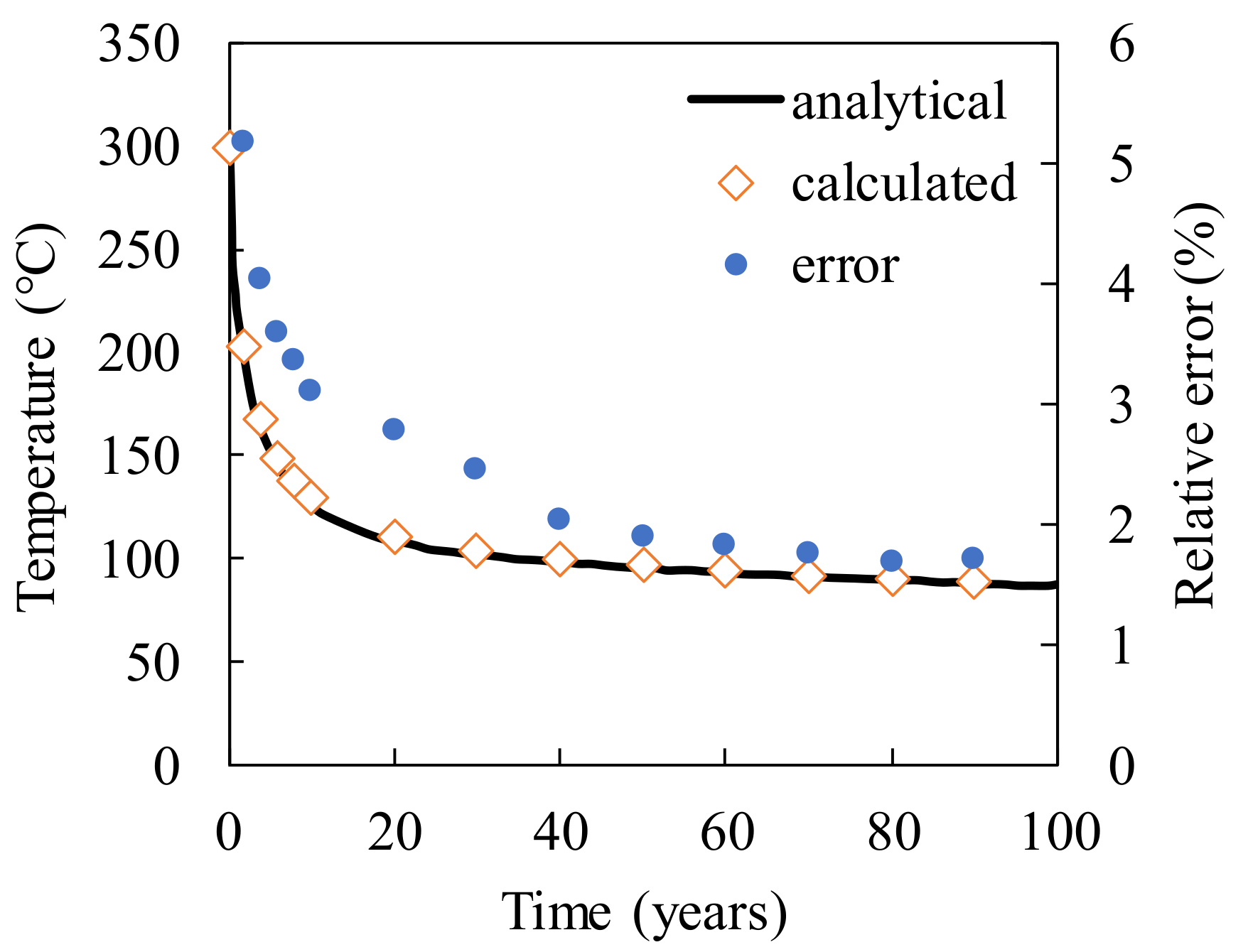
3. The Verification of the Mathematical Solution

A single fracture model is designed to compare the calculated temperature decline profiles with the analytical solution of Gringarten et al. [30]. The validation model consists of 1000 × 1000 m² in the x and y directions and the height of fracture is assumed to be 1000 m fully penetrating the formation. The 500 m spacing is sufficient to prevent the thermal front from reaching the boundary. The initial temperature of the rock is assumed to be 300 °C and cool water with a temperature of 65 °C is injected into the rock at a rate of 0.145 m³/s. The other properties are listed in

Table 1. The properties of rock and water used in the model verification.

Parameters	Value
Rock density	2.65 g/cm3
Water density	1.0 g/cm3
Rock thermal conductivity	2.595 × 10−2 J/(m·s·°C)
Rock specific heat capacity	1.05 J/(g·°C)
Water specific heat capacity	4.186 J/(g·°C)
Fracture porosity	1, decimal
Rock porosity	0, decimal

.

The calculated results compared with the analytical solution are shown in Figure 1. As shown in Figure 1, the calculated results match the analytical solution well, and the error curve is calculated as (calculated value-analytical value)/analytical value × 100, which indicates that the solutions from our work are reasonably accurate.

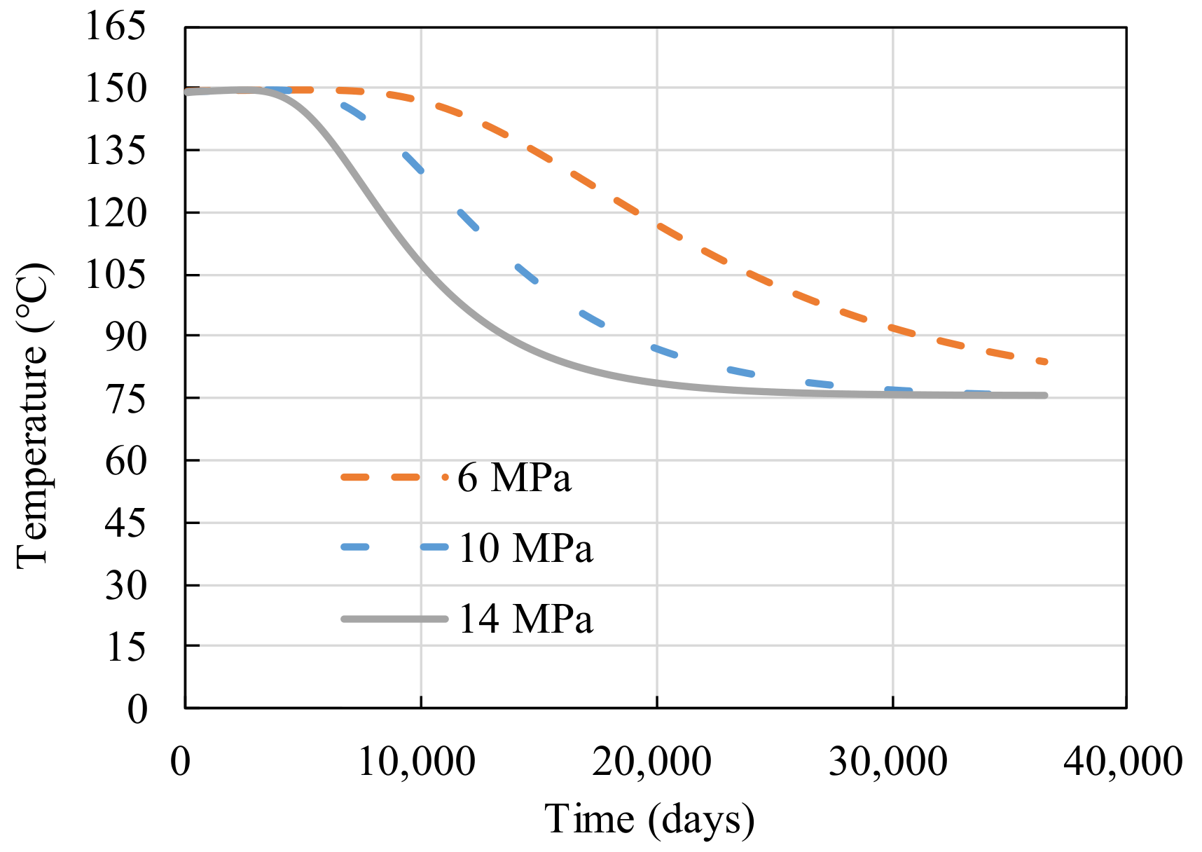
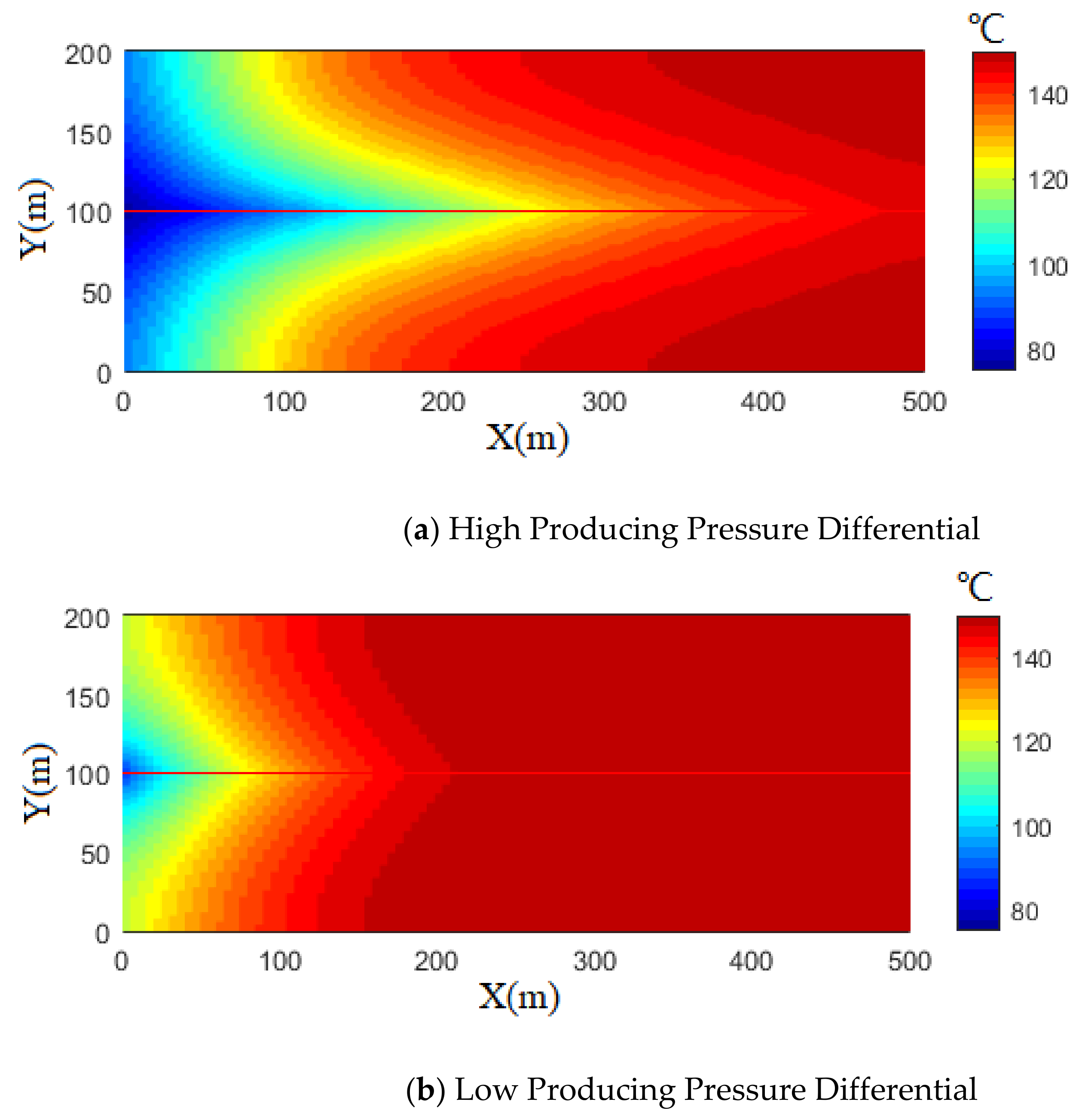
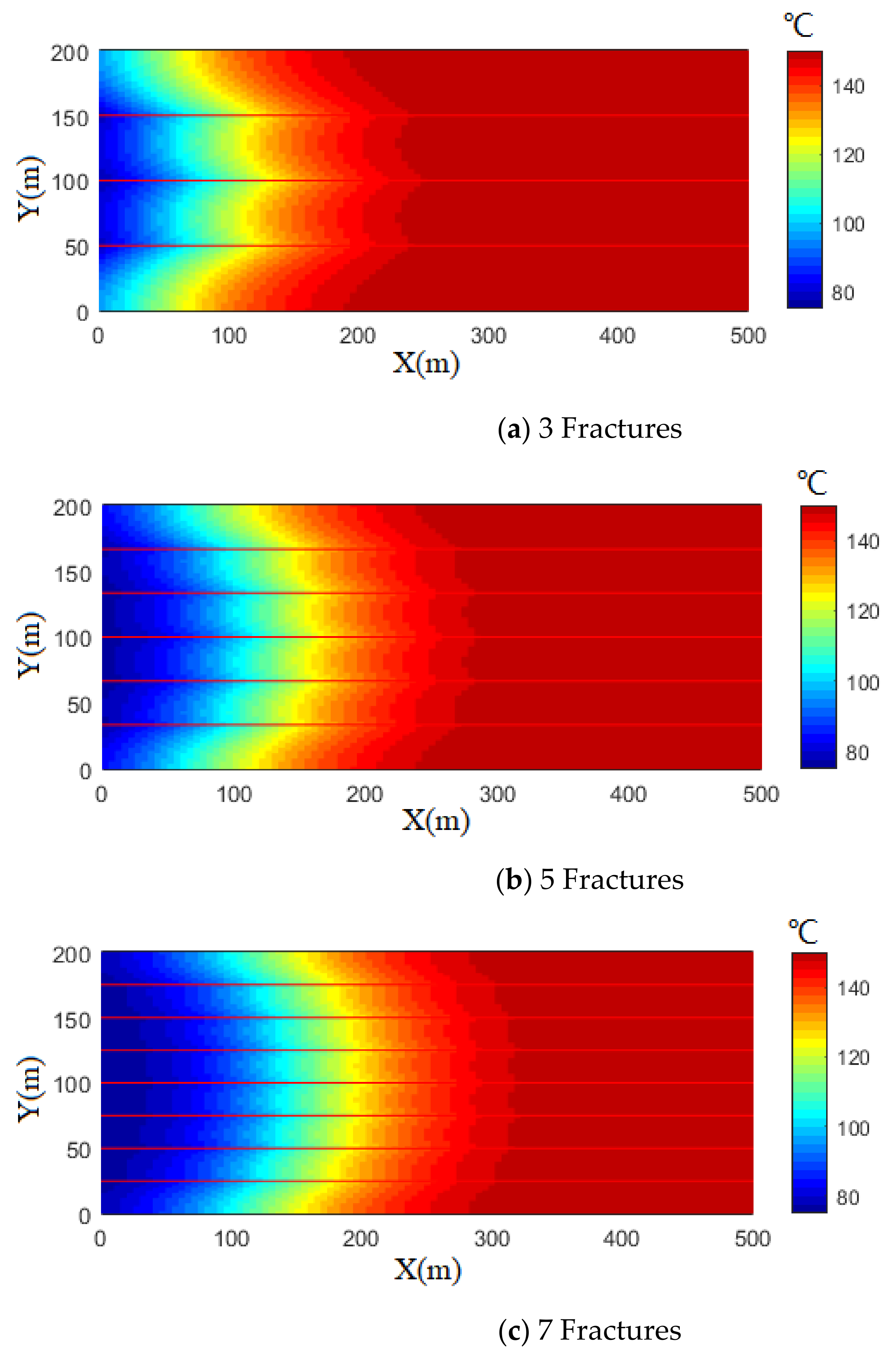
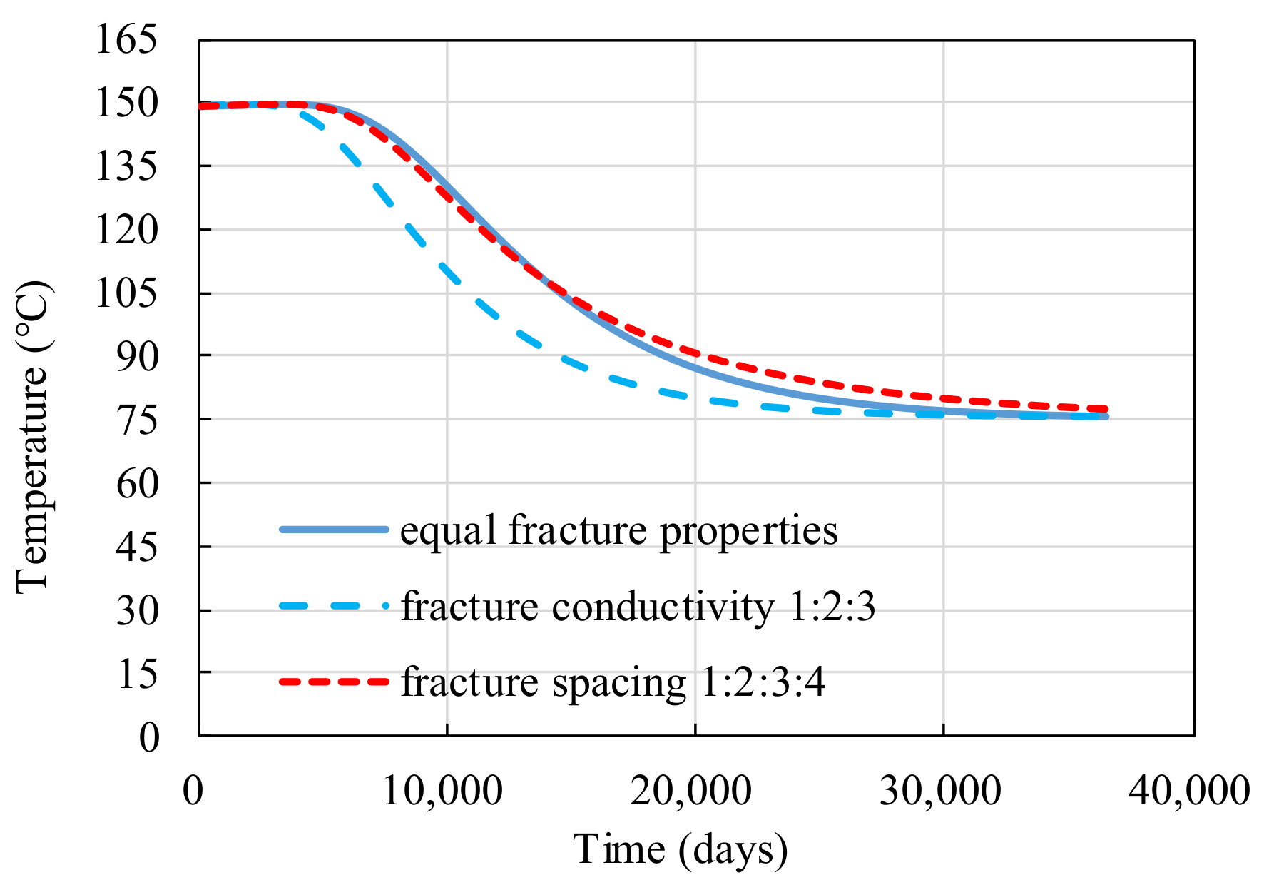
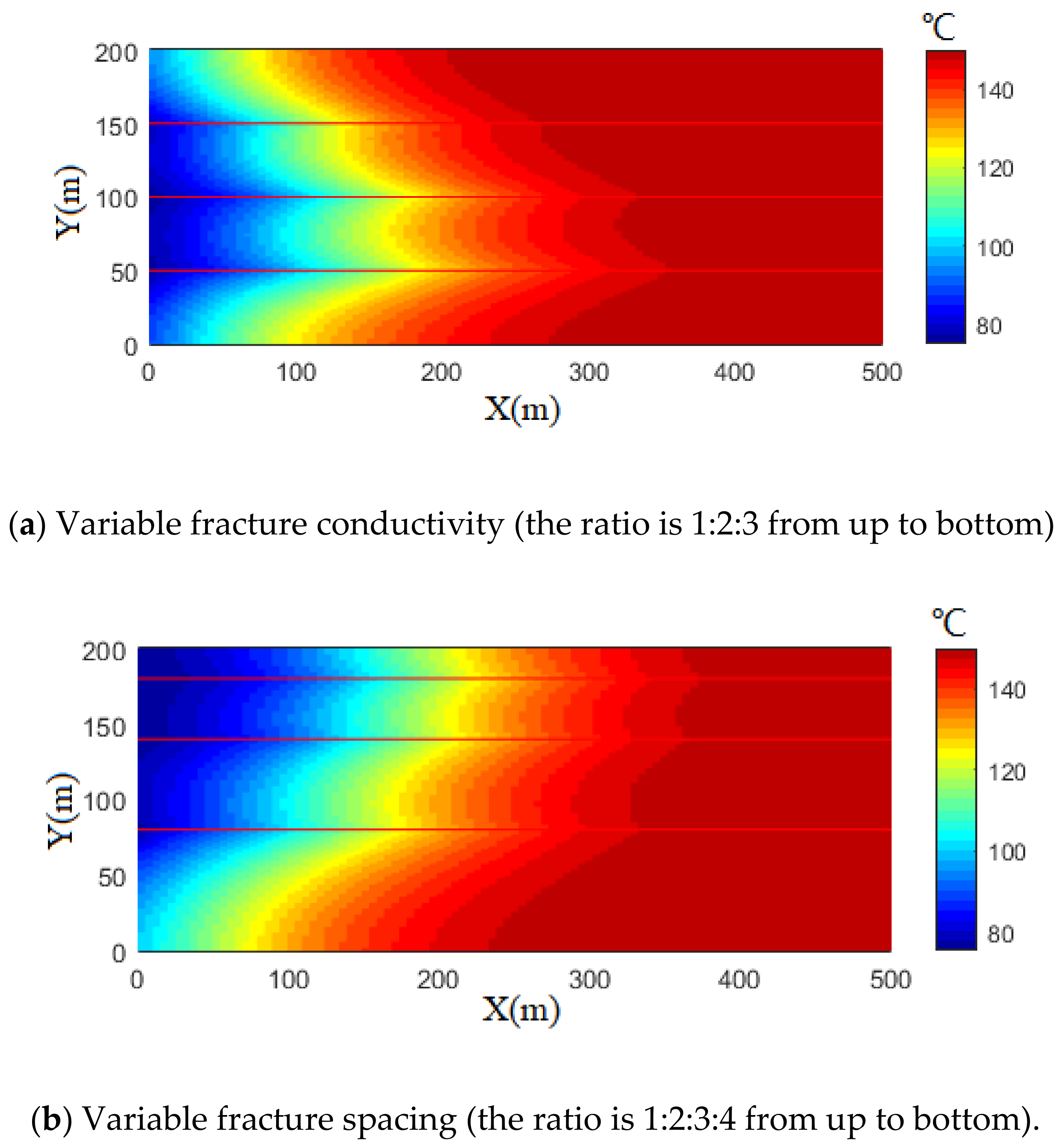
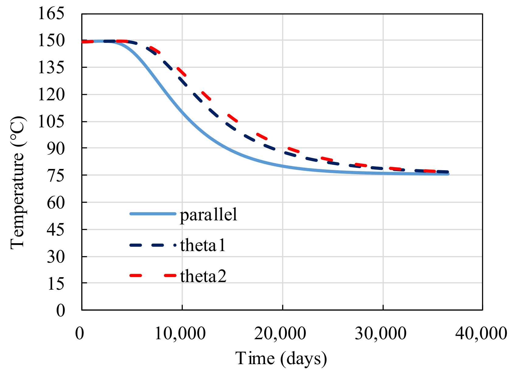
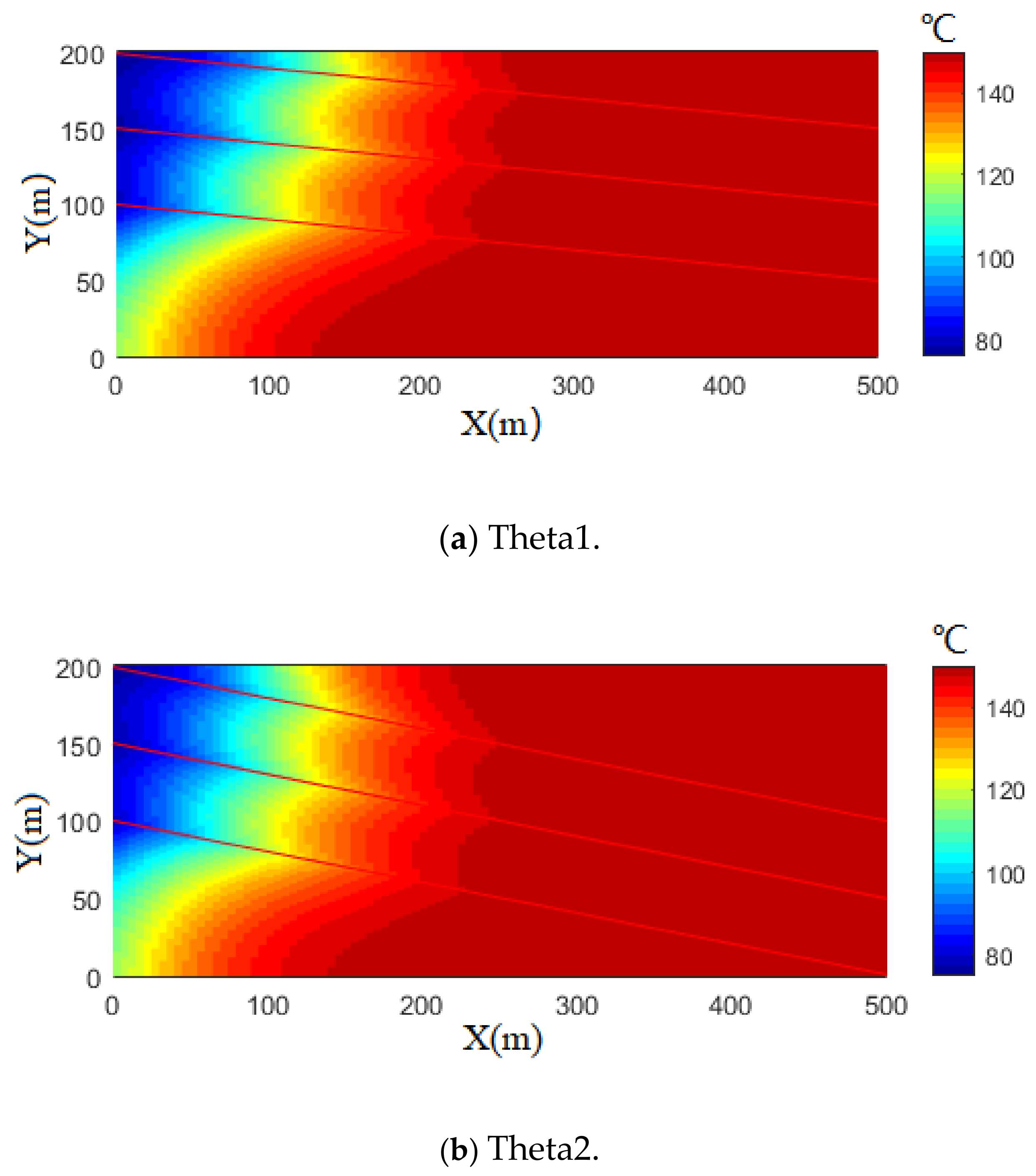
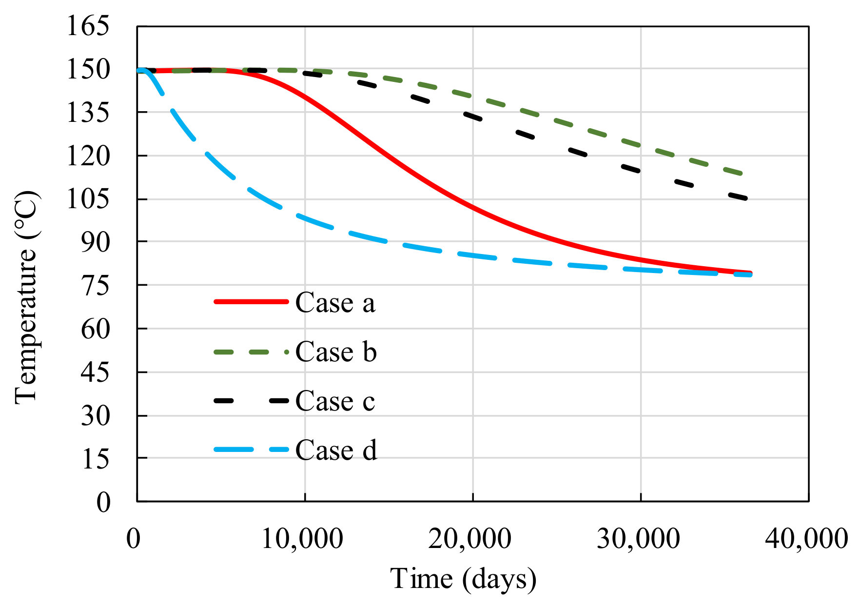
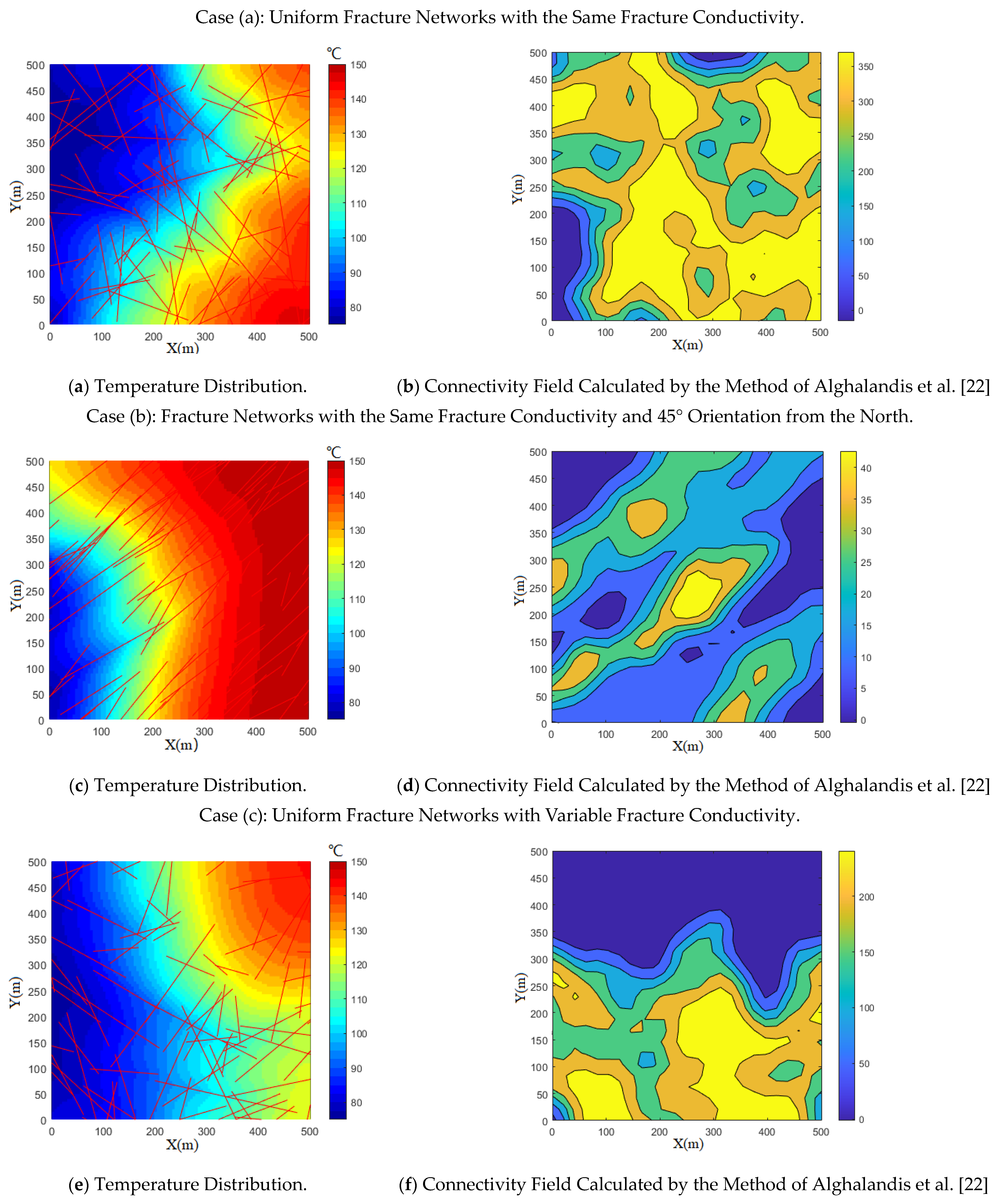
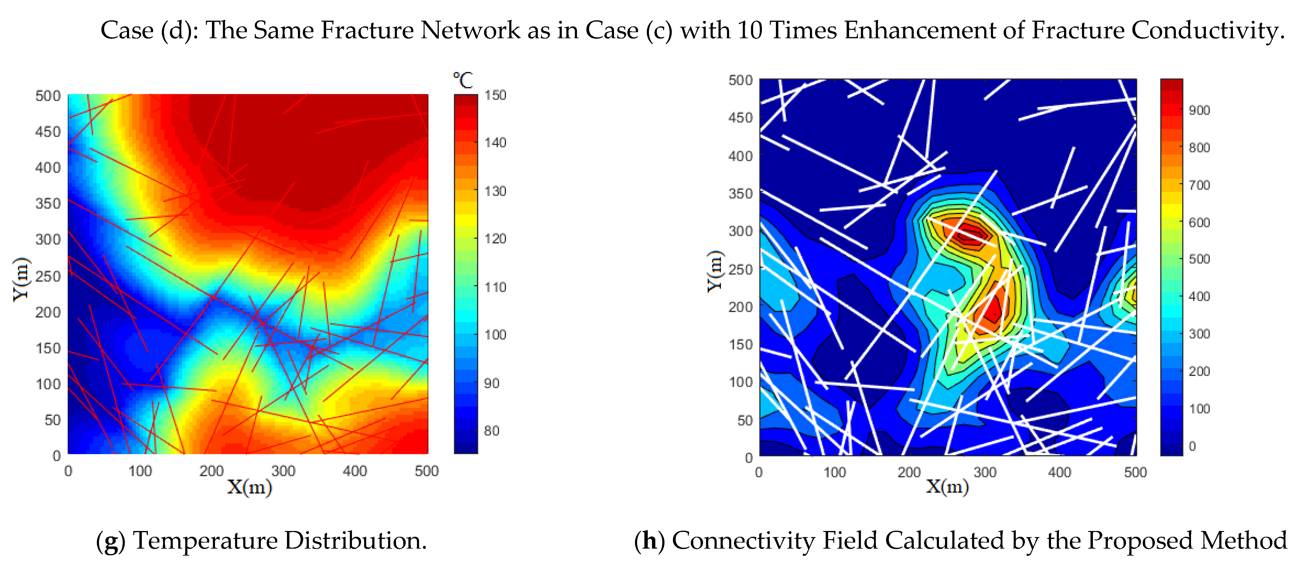
4. The Effects of Fracture Networks on the Heat Extraction Performance

In this section, a model of 500 × 200 m² is established to study the effects of fractures on heat extraction performance starting from regular distribution to complex fracture networks. In the model, two horizontal wells are set up at the opposite ends of the model for heat injection and production at the constant borehole pressure. Figure 2 and Figure 3 demonstrate the evolution of pressure and temperature for three evenly distributed fractures with the same fracture aperture. With the time proceeding, the cold water at first enters the fractures under the high injection pressure and the pressure within fractures is lower than that in the matrix. The pressure front spreads from the injection well to the production well. The temperature propagation shows fracture channeling. The thermal energy in the matrix conducts the cold water and flows along with fractures to the production well. The temperature of the rock is decreasing gradually to the temperature of injecting water at a later stage of production.

Figure 4 shows the temperature breakthrough curves at different producing pressure differentials. It indicates that the bigger pressure differential promotes the earlier temperature breakthrough. The temperature drops from the initial rock temperature to the temperature of the cold water.

To clearly show the effect of producing pressure differentials on thermal breakthrough, a single fracture model is established as shown in Figure 5. For the high-producing pressure differential, the thermal front in the fracture moves at a higher rate in the fracture than in the matrix. As the producing pressure differential becomes less, the thermal front in the matrix can keep up with that of the fracture. The higher-pressure differential leads to sharper thermal decline as shown in Figure 4.

As shown in Figure 6, under the same producing pressure differential, the increase in the number of fractures leads to a sharp thermal decline. That is because more fractures enhance the permeability of the rock matrix and high flow rate, which leads to an earlier breakthrough and less time for energy exchange between injected water and hot matrix. However, the difference in thermal breakthrough curves becomes less obvious with the increase in the fracture number. A high fracture intensity leads to thermal interference between the fractures. As indicated in Figure 7, the thermal front in the matrix is arriving almost at the same time as in the fractures for 7 fractures; the sharp decline in the thermal breakthrough curves reflects a high degree of thermal interference between fractures. Therefore, an increase in the fracture intensity has little influence on the thermal extraction.

The above cases are for homogeneous, constant spacing fractures with the same properties. Figure 8 and Figure 9 show the effects of variable fracture aperture and spacing on thermal breakthrough. The fracture conductivity and spacing are changed individually while keeping other parameters the same as the base model. The ratio of fracture conductivity is set to 1:2:3 counting from the upside of the model. The ratio of fracturing spacing separated by three fractures is 1:2:3:4 counting from the upside of the model. As shown in Figure 8, the heterogeneous distribution of fracture properties causes earlier and sharper thermal decline compared to fracture distribution with uniform spacing and conductivity. High fracture conductivity and intensity make the thermal front move quicker than the rest part, resulting in an earlier thermal breakthrough, as shown in Figure 9.

Figure 10 and Figure 11 show the effect of fracture direction on thermal breakthrough. It is obvious that an increase in the angle between flow direction and fracture orientation delays the thermal breakthrough and the fall-off of curves becomes less sharp.

Figure 12 and Figure 13 show the temperature distribution in complex fracture networks. The complex fracture networks are generated by an open-source software FracGen [18]. In this software, the fracture attributes of fracture networks (fracture center points, length, orientation, and aperture) are described by the corresponding probability density function. The connectivity of the fracture networks is controlled using an optimal algorithm. The fracture network in case (a) is generated using a uniform distribution of fracture center points and arbitrary fracture orientation. Fracture length follows an exponential distribution with the same fracture aperture. The fracture orientation in case (b) is set up at 45° from the north with the same fracture conductivity in case (a). Case (c) is generated using the same input parameters but with variable fracture conductivity. The fracture network in case (d) is as same as in case (c) with 10 times the original fracture conductivity in case (c). Figure 12 shows the thermal breakthrough curves for the different complex networks. There is not a very clear relationship between fracture networks and thermal production. The fracture network connectivity controls the flow characterization as mentioned in the introduction. Following the method of Alghalandis et al. [22], the connectivity field can be calculated according to the fracture network intersection.

As illustrated in Figure 13, for the uniformly distributed fracture network in case (a), the thermal front moves mostly equally and the connectivity field in the whole region seems homogenous. In case (b), the fracture orientation controls the flow characteristics, which follows the distribution of the connectivity field. In case (c), the variation of fracture conductivity leads to thermal channeling on the bottom part. The connectivity field also confirms the temperature field. Compared with the average value of the connectivity field from case (a) to case (c), the high value results in an early breakthrough in the thermal front as shown in Figure 12. However, in case (d), the fracture conductivity is enhanced 10 times, and due to the strong heterogeneity in fracture properties, the thermal flow path is very different from the case (c), although they have the same fracture networks. Compared with Figure 13f,g, The method proposed by Alghalandis is not suitable because the quantities associated with flow properties are not considered.

During the flow process, high fracture conductivity determines the flow path, and the flow rate is inversely proportional to the distance of injection well or production well. Furthermore, the flow is easier when away from the no-flow boundary. Therefore, based on the calculation of the connectivity field, a modified connectivity field correlation is proposed as follows:

$$\begin{gathered} \mathrm{CF}=\left\{\eta {\displaystyle \sum }_{i=1}^m{\displaystyle \sum }_{j=1}^{n}1\left(p_v\left(ij\right)\leftrightarrow q_v\left(ab\right)\right);a, b\in G\right\}·L\left(p_v\left(ij\right)\to noflow boundary\right) \\ {\log }_e\left\{L\left(p_v\left(ij\right)\to constant pressure boundary\right)\right\} , \end{gathered}$$

(21)

where $\eta$ is a normalization factor; $p_v\leftrightarrow q_v$ refers to that two supports (with size $\nu$ positioned at points $p$ and $q)$ are connected via fractures. One is the indicator for connected fractures. $L\left(p_v\left(ij\right)\to noflow boundary\right)$ refers to the distance between grid center and no-flow boundary. ${\log }_e\left\{L\left(p_v\left(ij\right)\to constant pressure boundary\right)\right\}$ refers to the natural logarithm of the distance between the grid center and constant pressure boundary.

The connectivity field is re-calculated as shown in Figure 13h, which shows that the shape of the connectivity contour matches well with the thermal flow path. The modified connectivity field can better describe the flow characteristic for complex fracture networks.

5. Discussion

The influences of pressure differential on the thermal breakthrough are discussed. Indeed, the variation of pressure differential changes the flow rate. Therefore, for the scenarios of constant injecting or producing rate, it can be inferred that the high fracture intensity will delay the thermal breakthrough because of a lower rate for each fracture. The variation of fracture conductivity has great effects on the temperature distribution and form thermal channeling to cause earlier time thermal breakthrough. As shown in Figure 13e, the variable fracture conductivity causes the thermal flow preferentially at the bottom part, and the connectivity field calculated by the method of Alghalandis et al. [22] has a high value at the bottom, which indicates more probability for thermal flow. However, when the fracture conductivity is enhanced 10 times at the basis of Figure 13e, the temperature field becomes very different, and an obvious cold temperature belt is across the study domain. The method proposed by Alghalandis et al. [22] only relies on the intersection information of fractures, not considering the flow properties of fractures. As shown in Figure 13h, the new connectivity field calculated by Equation (21) shows a high-value belt analogy to the temperature field. Therefore, the proposed method for connectivity field calculation including the fracture conductivity can infer the preferential thermal breakthrough path without mass thermal flow simulation. The above cases are based on the same conductivity with a single fracture. For the variable-conductivity fracture, it can be treated roughly as a series of short, connected fractures with the same conductivity. The proposed method can be also applied. It is useful in the optimization of drilling locations. The places with high values of modified connectivity field can be potentially suitable for well location, which provide the initial solution for optimal calculation of production performance.

6. Conclusions

A hydro-thermal coupling mathematical model is developed and validated considering complex fracture networks based on the EDFM method for EGS, and the effects of complex fracture from regular to complex geometries on the thermal breakthrough are investigated and a new method is proposed to calculate the connectivity field of fracture networks considering the effect of fracture conductivity on heat flow. The following conclusions are drawn:

(1) The increase in the producing pressure differential speeds up the thermal breakthrough by having a high flow rate. High fracture numbers will enhance mass flow and cause an early thermal breakthrough in the constant borehole pressure production. The increase in fracture number leads to thermal interference and little change in thermal extraction.

(2) The fracture network connectivity plays a key role in the mass flow and heat transfer, which controls the shape of thermal breakthrough curves. A modified connectivity field is proposed to better describe the flow path in complex fracture networks.

(3) The strong variation in fracture conductivity, as well as spacing and orientation, will cause thermal flow channeling and decrease the efficiency of heat extraction. Fracture networks with uniform conductivity will be better for heat extraction.

References

1. Blackwell, D.D.; Negraru, P.T.; Richards, M.C. Assessment of the Enhanced Geothermal System Resource Base of the United States. Nat. Resour. Res. 2007, 15, 283–308. [Google Scholar] [CrossRef]
2. Lu, S.-M. A global review of enhanced geothermal system (EGS). Renew. Sustain. Energy Rev. 2018, 81, 2902–2921. [Google Scholar] [CrossRef]
3. Song, X.; Shi, Y.; Li, G.; Yang, R.; Wang, G.; Zheng, R.; Li, J.; Lyu, Z. Numerical simulation of heat extraction performance in enhanced geothermal system with multilateral wells. Appl. Energy 2018, 218, 325–337. [Google Scholar] [CrossRef]
4. Sun, Z.; Xin, Y.; Yao, J.; Zhang, K.; Zhuang, L.; Zhu, X.; Wang, T.; Jiang, C. Numerical Investigation on the Heat Extraction Capacity of Dual Horizontal Wells in Enhanced Geothermal Systems Based on the 3-D THM Model. Energies 2018, 11, 280. [Google Scholar] [CrossRef] [Green Version]
5. Olasolo, P.; Juárez, M.C.; Morales, M.P.; Liarte, I.A. Enhanced geothermal systems (EGS): A review. Renew. Sust. Energ. Rev. 2016, 56, 133–144. [Google Scholar] [CrossRef]
6. Isaka, B.A.; Ranjith, P.G.; Rathnaweera, T.D. The use of super-critical carbon dioxide as the working fluid in enhanced geo-thermal systems (EGSs): A review study. Sustain. Energy Techm. 2019, 36, 100547. [Google Scholar]
7. Song, W.; Wang, C.; Du, Y.; Shen, B.; Chen, S.; Jiang, Y. Comparative analysis on the heat transfer efficiency of supercritical CO2 and H2O in the production well of enhanced geothermal system. Energy 2020, 205, 118071. [Google Scholar] [CrossRef]
8. Li, J.; Yuan, W.; Zhang, Y.; Cherubini, C.; Scheuermann, A.; Torres, S.A.G.; Li, L. Numerical investigations of CO2 and N2 miscible flow as the working fluid in enhanced geothermal systems. Energy 2020, 206, 118062. [Google Scholar] [CrossRef]
9. Karmakar, S.; Ghergut, J.; Sauter, M. Early-flowback tracer signals for fracture characterization in an EGS developed in deep crystalline and sedimentary formations: A parametric study. Geothermics 2016, 63, 242–252. [Google Scholar] [CrossRef]
10. Ma, Y.; Li, S.; Zhang, L.; Liu, S.; Liu, Z.; Li, H.; Shi, E.; Zhang, H. Numerical simulation study on the heat extraction performance of multi-well injection enhanced geothermal system. Renew. Energy 2020, 151, 782–795. [Google Scholar] [CrossRef]
11. Cipolla, C.L.; Lolon, E.P.; Erdle, J.C.; Rubin, B. Reservoir Modeling in Shale-Gas Reservoirs. SPE Reserv. Eval. Eng. 2010, 13, 638–653. [Google Scholar] [CrossRef]
12. Mukuhira, Y.; Ito, T.; Asanuma, H.; Häring, M. Evaluation of flow paths during stimulation in an EGS reservoir using micro-seismic information. Geothermics 2020, 87, 101843. [Google Scholar] [CrossRef]
13. Chilès, J.P. Fractal and geostatistical methods for modeling of a fracture network. Math. Geol. 1988, 20, 631–654. [Google Scholar] [CrossRef]
14. Davy, P.; Sornette, A. Some consequences of a proposed fractal nature of continental faulting. Nat. Cell Biol. 1990, 348, 56–58. [Google Scholar] [CrossRef]
15. Darcel, C.; Bour, O.; Davy, P.; De Dreuzy, J.R. Connectivity properties of two-dimensional fracture networks with stochastic fractal correlation. Water Resour. Res. 2003, 39, 39. [Google Scholar] [CrossRef]
16. Kim, T.H.; Schechter, D.S. Estimation of Fracture Porosity of Naturally Fractured Reservoirs With No Matrix Porosity Using Fractal Discrete Fracture Networks. SPE Reserv. Evaluation Eng. 2009, 12, 232–242. [Google Scholar] [CrossRef]
17. Xu, C.; Dowd, P. A new computer code for discrete fracture network modelling. Comput. Geosci. 2010, 36, 292–301. [Google Scholar] [CrossRef]
18. Boyle, E.J.; Sams, W.N. NFFLOW: A Reservoir Simulator Incorporating Explicit Fractures. In Proceedings of the SPE Western Regional Meeting, Bakersfield, CA, USA, 19–23 March 2012. [Google Scholar]
19. La Pointe, P. A method to characterize fracture density and connectivity through fractal geometry. Int. J. Rock Mech. Min. Sci. Géoméch. Abstr. 1988, 25, 421–429. [Google Scholar] [CrossRef]
20. Berkowitz, B. Analysis of fracture network connectivity using percolation theory. Math. Geol. 1995, 27, 467–483. [Google Scholar] [CrossRef]
21. Xu, C.; Dowd, P.A.; Mardia, K.V.; Fowell, R.J. A Connectivity Index for Discrete Fracture Networks. Math. Geol. 2006, 38, 611–634. [Google Scholar] [CrossRef]
22. Alghalandis, Y.F.; Dowd, P.A.; Xu, C. Connectivity Field: A Measure for Characterising Fracture Networks. Math. Geol. 2014, 47, 63–83. [Google Scholar] [CrossRef]
23. Li, L.; Jiang, H.; Wu, K.; Li, J.; Chen, Z. An analysis of tracer flowback profiles to reduce uncertainty in fracture-network ge-ometries. J. Petrol. Sci. Eng. 2019, 173, 246–257. [Google Scholar] [CrossRef]
24. Barenblatt, G.; Zheltov, I.; Kochina, I. Basic concepts in the theory of seepage of homogeneous liquids in fissured rocks [strata]. J. Appl. Math. Mech. 1960, 24, 1286–1303. [Google Scholar] [CrossRef]
25. Warren, J.; Root, P. The Behavior of Naturally Fractured Reservoirs. Soc. Pet. Eng. J. 1963, 3, 245–255. [Google Scholar] [CrossRef] [Green Version]
26. Pruess, K.; Narasimhan, T.N. A practical method for modeling fluid and heat flow in fractured porous media. SPE J. 1982, 25, 14–26. [Google Scholar] [CrossRef] [Green Version]
27. Sarda, S.; Jeannin, L.; Basquet, R.; Bourbiaux, B. Hydraulic Characterization of Fractured Reservoirs: Simulation on Discrete Fracture Models. SPE Reserv. Eval. Eng. 2002, 5, 154–162. [Google Scholar] [CrossRef]
28. Karimifard, M.; Durlofsky, L.J.; Aziz, K. An Efficient Discrete-Fracture Model Applicable for General-Purpose Reservoir Simulators. SPE J. 2004, 9, 227–236. [Google Scholar] [CrossRef]
29. Li, L.; Lee, S.H. Efficient Field-Scale Simulation of Black Oil in a Naturally Fractured Reservoir Through Discrete Fracture Networks and Homogenized Media. SPE Reserv. Eval. Eng. 2008, 11, 750–758. [Google Scholar] [CrossRef]
30. Gringarten, A.C.; Witherspoon, P.A.; Ohnishi, Y. Theory of heat extraction from fractured hot dry rock. J. Geophys. Res. Space Phys. 1975, 80, 1120–1124. [Google Scholar] [CrossRef]
31. Doe, T.; McLaren, R.; Dershowitz, W. Discrete fracture network simulations of enhanced geothermal systems. In Proceedings of the Thirty-Ninth Workshop on Geothermal Reservoir Engineering Stanford University, Stanford, CA, USA, 24–26 February 2014; pp. 24–26. [Google Scholar]
32. Gan, Q.; Elsworth, D. Production optimization in fractured geothermal reservoirs by coupled discrete fracture network mod-eling. Geothermics 2016, 62, 131–142. [Google Scholar] [CrossRef] [Green Version]
33. Gong, F.; Guo, T.; Sun, W.; Li, Z.; Yang, B.; Chen, Y.; Qu, Z. Evaluation of geothermal energy extraction in Enhanced Geothermal System (EGS) with multiple fracturing horizontal wells (MFHW). Renew. Energy 2020, 151, 1339–1351. [Google Scholar] [CrossRef]
34. Asai, P.; Panja, P.; McLennan, J.; Moore, J. Efficient workflow for simulation of multifractured enhanced geothermal systems (EGS). Renew. Energy 2019, 131, 763–777. [Google Scholar] [CrossRef]
35. Asai, P.; Panja, P.; McLennan, J.; Moore, J. Performance evaluation of enhanced geothermal system (EGS): Surrogate models, sensitivity study and ranking key parameters. Renew. Energy 2018, 122, 184–195. [Google Scholar] [CrossRef]
36. Peaceman, D.W. Interpretation of well-block pressures in numerical reservoir simulation with nonsquare grid blocks and ani-sotropic permeability. SPE J. 1983, 23, 531–543. [Google Scholar]
37. Lie, K.A.; Krogstad, S.; Ligaarden, I.S.; Natvig, J.R.; Nilsen, H.M.; Skaflestad, B. Open-source matlab implementation of con-sistent discretisations on complex grids. Comput. Geosci. 2012, 16, 297–322. [Google Scholar] [CrossRef] [Green Version]
38. Lie, K.A. An Introduction to Reservoir Simulation Using MATLAB/GNU Octave: User Guide for the MATLAB Reservoir Simulation Toolbox (MRST); Cambridge University Press: Cambridge, UK, 2019. [Google Scholar]
Figure 1. Comparison between the calculated and Gringarten’s analytical solution.
Energies 14 01635 g001
Figure 2. The pressure distribution marked by color (pictures on the left side) and contour (pictures on the right side) at different times (T3 > T2 > T1). Compared with (ac), water flows preferentially in fractures and a high-pressure drawdown occurs in fractures at first. The contour is curved. With the time advancing, the pressure in matrix starts to drop and the contour becomes more parallel in the later time.
Energies 14 01635 g002
Figure 3. The temperature distribution marked by color (pictures on the left side) and contour (pictures on the right side) at different times (T3 > T2 > T1). Compared with (ac), the temperature falls off firstly in the fractures and the temperature difference between fractures and matrix becomes less with the time advancing. Finally, the temperature in matrix approaches the injection temperature.
Energies 14 01635 g003aEnergies 14 01635 g003b
Figure 4. Effect of producing pressure differential on thermal breakthrough.
Energies 14 01635 g004
Figure 5. Thermal front comparison between high and low producing pressure differential. Compared with (a,b), the high producing pressure differential makes the thermal front spread quicker than that in the matrix.
Energies 14 01635 g005
Figure 6. Effect of fracture number on thermal breakthrough.
Energies 14 01635 g006
Figure 7. Thermal front for different fracture numbers. Compared with (ac), the thermal front in the matrix and fractures is arriving almost at the same time when the number of fractures increase.
Energies 14 01635 g007
Figure 8. Thermal breakthrough for variable fracture conductivity and spacing.
Energies 14 01635 g008
Figure 9. Temperature distribution for variable fracture conductivity and spacing. For the (a), the thermal front spreads firstly in the high-condcutivity fracture. For the (b), the small fracture spacing leads to early thermal breakthrough.
Energies 14 01635 g009
Figure 10. Effect of fracture orientation on thermal breakthrough.
Energies 14 01635 g010
Figure 11. Temperature distribution for different fracture orientations (theta1 < theta2). Conpared with (a,b), an increase in the angle between flow direction and fracture orientation delays the thermal breakthrough.
Energies 14 01635 g011
Figure 12. Thermal breakthrough curves for different fracture networks.
Energies 14 01635 g012
Figure 13. Temperature distribution and connectivity field for complex fracture networks. (a,c,e,g) is the temperature distribution. (b,d,f,h) is the fracture-network connectivity filed. (a,b) are for uniform fracture networks with the same fracture conductivity. (c,d) are for fracture networks with the same fracture conductivity and 45° orientation from the north. (e,g) have the same fracture networks, however, the fracture conductivity in (g) is 10 times than that in (d).
Energies 14 01635 g013aEnergies 14 01635 g013b