1. Introduction
Through the years, the number of electric vehicles (EV) has significantly increased all over the world. There is a growth projection of 250 million EVs by 2030 [
1,
2,
3]. Alongside the EV growth, the number of electric vehicles charging stations (EVCS) hand increased by 44% from 2018 to 2019 [
3]. Most of EVCS are based on private investments [
1]. Although the growth of EV, and furthermore EVCS, could present environmental benefits, an uncoordinated penetration may present problems to power grid performance. These problems are related to the following: peak demands higher than the distribution system operator (DSO), voltage distortions, overloading of lines, and another energy quality problem [
4,
5,
6]. Knowing these problems, the EVCS management relates to carefully select the charging time and quantity for EV use. This management could maximize economic benefits and reduce grid impact.
Related to EVCS management, a common approach is focused on demand shifting, applying controls over the EV charging and discharging [
7,
8,
9,
10,
11]. The work of Reference [
12] focuses on maximizing the number of EV charges at the station, respecting the grid limits of the DSO. Furthermore, metaheuristic (MH) techniques are presented as valid solutions, as they offer flexibility and simplicity of implementation. An example of MH is presented in Reference [
9], where a genetic algorithm (GA) is used to flatten daily loading curves. The authors of Reference [
7] showed that the particle swarm optimization (PSO) technique performed better than the GA method when scheduling consumer charging. In addition, Reference [
13,
14] applies a PSO algorithm for solution based on planning strategies. In Reference [
15], a framework solution for EVCS planning is developed, considering interactions between EV and EVCS. The framework is based on long term evaluation and rules to check charging demands and EV growth towards rejections indices and locations.
In addition to load management methods, the use of distributed energy resources (DERs) could support the EVCS by reducing dependence on grid power. Normally, DERs are composed of renewable energy sources, such as wind or solar photovoltaic (PV) generation and/or battery energy storage systems (BESS). Adding these factors makes the EVCS management more challenging and brings complexity for the operation. In Reference [
10], DERs are considered in energy management control (EMC) system, using BESS lifetime as a factor to minimize total operational costs. The work of Reference [
16] also considers PV generation but focuses on residential EV use. In Reference [
16], the BESS stores PV energy surplus to be injected into the grid or residence. In Reference [
17], an EV scheduling approach based on a Markov Decision Process (MDP) is proposed. In Reference [
17], the main objective is to minimize the average waiting time of EVs and considers charging stations having renewable energy generators and storage devices at disposal. In Reference [
18], a solution for BESS support on EVCS is developed, considering wind farm as renewable resource. A genetic algorithm is applied for optimization but disregards EV scheduling and EV chargers availability and types.
It should be noted that EVCS operation problem depends on different objectives, as there is participation of several agents. As mentioned, there is a necessity to balance both the EVCS interest on increasing the EV chargings without compromising the DSO interest on reducing the stress on the grid caused by possible overloadings. Moreover, it is also important to consider the user comfort in terms of waiting times and charging speed. Regarding this, some scheduling models are based on selection of time periods for charging by the users. In Reference [
19], an application was developed allowing the EV owner to pick an EVCS location, based on its necessities. A machine learning approach [
8] was applied to select chargers options for the users.
As EVCS investment is gaining interest, some applications further expand to long distance travel, in contrast to the short and common EV trips inside cities [
20]. As an example, the EV Charging Station installed at the COPEL-Distribution Electric Power Company in the Curitiba City—Paraná—Brazil will further extend a larger electrovia that communicates several cities [
21]. Large distance travel gives more challenges as the EV requires an adequate availability for charging. In addition, times for charging should be short in order to optimize EV travel. The use of scheduled methods is important for EVCS for adequately manage the chargers to attend demand based on previous information.
Considering EV stochastic behavior, predictive analysis could be useful for charging planning [
17,
22]. Nevertheless, the need for information to construct forecast data could be a limitation for new infrastructure investment. An alternative to gain information is previous scheduling based on request for EV users, interested in charging for future use. For this approach, the previous cited heuristic techniques and frameworks [
7,
17,
19,
23,
24,
25,
26], are useful to schedule the charging operation. However, real time operation gets limited if there is a lack of information for new users. In addition, difference in distance from arriving to the station could impact the charging time. Therefore, rule-based (RB) strategies are presented as an alternative solution. RB strategies [
7,
10,
25,
27] are based on decision-making choices considered set of conditions and depending on present information. Thus, a combination of schedule planning, with real time operation, could give a more robust operation for EVCS focus on EV user comfort, DSO objectives, and EVCS profit.
This paper proposed an MH technique combined with RB framework for EVCS operation, considering PV and BESS support. The heuristic chosen was an evolutionary particle swarm optimization algorithm (EPSO), in which the present rapid convergence is less sensitive to parameters changes as PSO [
28]. The proposed work is denoted as EPSO-RB, to combine the two techniques. As intended for application in long distance travel, EVCS are located on highways. The charger’s characteristics are based on fast charging (30 min to 1:30 min), with 3 type of chargers. A comparison of EPSO-RB features against previous work is presented in
Table 1.
As shown by
Table 1, only EPSO-RB considered the key features presented. Thus, the main contributions of this work are:
A combined MH and RB technique for EVCS management considering scheduled and real time demands.
A method for EVCS management applied for long distance travel, considering short time of charging and BESS and PV support.
Multi-objective load shifting of EV applying an EPSO approach. Objectives set to economic profit and reduction on grids impact.
Real time-based framework for BESS support of EVCS considering degradation cost and PV injection.
RB strategy to handle difference on charging schedule and state of charge (SoC) variation for user arrival.
The work is divided as follows. First, a description of the methodology is explained. Second, a study case is made based on stochastic scenarios for representation of user’s demand. Finally, conclusions, about EPSO-RB impact are presented.
2. Proposed Methodology
The proposed EPSO-RB framework is based on two parts:
first, a day-ahead planning of EV users chargings is made based on the EPSO algorithm and the scheduling requests; and,
second, the RB strategy is used to manage the EVCS operation in real time. RB supports the EPSO planed load and the random load that may arrive during the day.
The model considers three types of charging modes. The first one is the Normal Charging (NC) that fully recharges the EV in 1 h and 30 min. The second type is the Fast Charging (FC) that takes 1 h to complete an EV charge. Finally, the Ultra-Fast Charging (UFC), that fully recharges an EV in 30 min. For each charging type, it is considered that the lower the time to complete the recharge the higher the price for sell. Taking FC chargers as reference, NC will be 10% cheaper, and UFC will be 10% more expensive. The model works in a time step (TS) of 30 min for each day, and the simulations are performed in Python programming language [
33]. It should be noted that the proposed approach was tested in only one EVCS, as the intention was for private and long distance applications. Nevertheless, the model could be adapted to consider more EVCS by establishing a communication and set of rules to attend multiple agents objectives.
2.1. Demand Model
The EVCS serves two different consumer types: The scheduled consumer (SCh) and the non-scheduled consumer (NSCh). For simplification purposes, all EV fleets have the same EV model, with a 40-kWh battery.
2.1.1. SCh Model
The SCh requests its own recharge by contacting the EVCS in the day before the recharge. Then, the consumer must provide to the EVCS the desired charging mode and the expected traveled distance before the arrival. The model associates this expected distance with the EV SoC to have a more accurate estimate of the required energy by the EV at the arrival.
Although the user cannot provide a specific time for the connection, they can still choose to request a recharge according with the cluster time that better suits his needs. These clusters are presented in
Table 2.
Table 2 shows 7 options for chargers vacancies, starting at time
and finishing at time
. As an example, if an EV owner wants to recharge his car at night, he should select, for instance, the cluster C6 (21:00 to 0:00) and then contact the EVCS on the day before. The range of time for the contact must be the same of the cluster, i.e., 21:00 to 0:00.
By the end of the selected cluster, the EVCS informs the EV owner about his scheduled time (or availability) for connection. It should be noted that the user will not be scheduled outside the chosen cluster time range for the studied case.
The clusters division is important to ensure user comfort. If the range for schedule is too long, this could provide long waiting times and uncertainty for the user request. Thus, the clusterization provides:
Due the lack of practical data on EV demand profile, a random distribution of EV users and profiles are generated.
Figure 1 shows the distribution of data for the EV users adapted from Reference [
34].
The histograms of
Figure 1 are used to generate the amount of EV users to be scheduled in each cluster by the EPSO algorithm. The green part in
Figure 1a represents the Commercial Period (CP) where the EVCS can supply both NSCh and SCh consumers. Outside the time window marked in green, only the SCh consumer can be supplied. The vertical lines denote the area of each cluster presented in
Table 2.
The SCh import of data by the ECVS is divided in two parts. First, each EV consumer selects his charging mode. Second, each EV consumer estimates the remaining movement capacity (km related to SoC use) upon arrival to EVCS.
Figure 2 presents the process of the first step. Note that, in
Figure 1b, the idea of having a larger number of EVs at a high SoC during the request time is to represent the consumers that, in the day before the recharge, will use the EV for traveling long distances, arriving at the EVCS with a lower SoC to then fully complete the recharge and to continue their trips.
In
Figure 2, for every EV evaluated at the current time step (TS), there is an associated SoC and probability to select a specific charging mode, depending in the SoC value. The set of rules created were defined by the authors to handle several scenarios, and the main idea of this set of probabilities is to bias the user to select a fast charging type if the required energy is low, a slow charging type if he needs a higher amount of energy, and the normal charging if its SoC is medium. The second process is represented in
Figure 3.
Figure 3 presents the determination process of the remaining SoC at arrival for the EV. This process depends on whether or not the consumer will use the EV before going to the EVCS. The estimation of this value is used on the EPSO algorithm. Then, the real SoC is handled on the RB strategy. The EV estimation is based on two factors:
first, the distance between the EV and the EVCS; and,
second, the expected usage of the EV before arrival at the EVCS.
For instance, if the EV owner has, at the time of the request, 40% of SoC, then the required amount of energy is 60% of the capacity. Nevertheless, if the user intends to use the EV before the recharge, he also must estimate the number of kilometers he will travel. The estimated value—based on the average consumption per kilometer of the EV—provides a more accurate estimated value for the SoC at arrival.
These estimates help the EVCS to better supply the EV and to dispatch its own DERs. In addition, the EV user is not penalized when the error between the estimate and the real energy is below 15%. If the error is above 15%, a penalization of 5% in the final EV consumer bill is applied. As the SCh user is responsible to give a realistic estimate on the expected EV usage before the recharge happens, this penalization is set to avoid losing performance at the EPSO scheduling because a very bad estimate could invalid the whole scheduled for a given cluster TS. Moreover, this penalization is only applied to the SCh consumer, as this consumer is the user who also does not need to request a schedule, and he canalso arrive at the EVCS as an NSCh consumer in order to recharge; however, if there is no available chargers, he would also have to wait until one of them is, and he cannot select its connection time in the day before.
Due to the limited number of chargers in the EVCS, for each cluster, there is also a limited number of reserves that can be made for each type of charging mode. For instance, the total number of UFC requests that can be scheduled in one single charger is eight if the selected cluster has 4 h of range because the UFC can completely recharge an EV in just 30 min.
Table 3 presents the total amount of schedules for each charging mode for each cluster.
2.1.2. NSCh Consumer
The NSCh consumer can only recharge their own vehicle if there is an available charger. However, this type of consumer can only arrive in the EVCS during the Commercial Period (CP), i.e., by 7:00 to 9:00. Outside this range, the EVCS will serve only the SCh consumer. The reason for this is to give some advantage to the SCh consumer, which in turn allows a better control for the EVCS dispatch.
For the study case, the NSCh consumers are randomly settled based on the histograms of
Figure 4. As NSCh works in real time, the EVCS has complete knowledge of the EV SoC at arrival, so there is no need for estimation.
Although the NSCh consumer depends on an available charger at arrival, he also can use the remaining chargers from the Scheduled process that have not been reserved. This approach maximizes the Scheduled chargers usage and extend availability for NSCh consumers to recharge.
2.2. EPSO Approach
The scheduled framework is based on the Evolutionary Particle Swarm Optimization (EPSO) method. This method relies on a self-adaptative technique analog to evolutionary behaviors. The EPSO defines a set of particles that represent a possible solution for the scheduling of the EV users. A random population is defined initially for the set of solution. In the search space, each particle presents a movement and to avoid unfeasible solutions a population ranking approach is used to select valid candidates. This algorithm is defined as follows [
28,
35]:
2.2.1. EPSO Contextualization
The EPSO approach share most parts of the PSO method [
26,
36,
37]. The particle movement follows rules based on inertia, memory, and cooperation; however, it can be said that it represents a self-adaptive algorithm because it uses concepts of mutation and selection of parameters.
The particle movement is presented in Equation (
1), where
is a particle,
is the new, and
is the particle velocity. Equation (
2) presents the velocity equation [
28].
where, in Equation (
2), the weights
are mutated based on a Gaussian distribution with mean 0 and variance 1, as presented in Equation (
3). The variable
b represents the best point found by the particle, and
is the global best point. The EPSO approach also replicates each particle
r times and mutates
in order to produce some disturbance [
28].
2.2.2. Population Ranking Process
Each individual must satisfy the constraint of maximum allowed EV connections for each TS. For instance, if the total amount of chargers is ten, then the total number of EV being recharged simultaneously is ten.
A feasible solution is based on a Mixed Integer Linear Programming (MILP) model, described as follows:
subject to
where, in Equation (
4),
,
, and
are the number of charging mode types scheduled for a specific charger
i. The Objective Function (OF) of Equation (
4) is defined to find a viable solution that satisfies the restrictions from Equations (
5) to (
8). The sum of all charging mode types in each charger must be equal to
,
, and
, which represents the total amount of schedules for
,
, and
, respectively.
In Equation (
5), the constants multiplying the variables
,
, and
refer to the number of TSs required by each charging type, considering the TS length of 30 min of this study.
In other words, the MILP problem is to find a setup where all the demanded charging types are assigned to some chargers without violating the total amount of available chargers. The
variable is the total amount of TSs in the cluster, which can be either eight (4 h) or six (3 h), as presented in
Table 2.
The MILP solution then provides a matrix that correlates charging types to chargers, and the final step is to randomly fill these chargers with the appropriated EVs. The final solution is then sent to the EPSO algorithm as a valid individual in the initial population. It should be noted that, for each generation, this solution could be improved by another individual; moreover, this approach avoids non-feasible solutions at the end of the algorithm.
2.2.3. EPSO Fitness Function Evaluation
In this study, the EVCS scheduling problem is approached by using the load shifting technique, and it is based on Reference [
35]. It is also considered that the operating day is discretized in
M TSs. The total number of EVs are
N, and they can be connected to the EVCS only once throughout the day. Moreover, the EV then must be charged during
consecutive TSs from its initial operation moment
. To assess the performance of each particle, a Fitness Function is applied and defined as:
where Equation (
9) represents the multi objective function for the EV scheduling.
w is the weight of the function
that represents the cost of supplying the load defined by:
where,
is a vector of dimension
that represents all the demanded power of the EVs (in kW) and is expressed as:
;
is a vector of dimension
in which the values represent the energy cost for each interval of time (in USD/kWh) and is expressed as:
;
is a binary matrix in which entries are the intervals where each EV remains connected or not. The inputs of
can have the value of 1 to indicate the EV
n is charging during the time
m, or the value of 0 if the EV is not charging in that moment.
Each EV have its own characteristics and stays connected to a charger by a specific and continuous interval sequence, according to the type of charging mode selected. The number of intervals that the charger will be at use is represented by
, while
represents the initial instant of operation of each charger, as shown below:
The second part of Equation (
9) is
, which represents the peak to average to peak to ratio (PAPR) metric. This metric seeks to secure better control and load reduction at the grid; lower values of PAPR means the system have a more plain load curve, which in turn limits the peaks and possible high grid purchases. In addition, with a lower peak, it is possible to control better the dispatch. Regarding the system performance variability, the RB strategy helps to handle in time events. Whenever the system needs, the RB relies on the grid support. The PAPR metric is defined as:
where
is the peak power over the
M scheduling TSs, and
is the mean value of the power among all the TSs. The variable
and
are presented, respectively, in Equations (
12)–(
13).
As presented in Equation (
9) both
and
are linearly combined through the weighted sum of them. When
w is unitary, the modeling will only consider the
metrics that are related to the costs for the EVCS. And, when
, only
is considered, giving more importance in the grid exchanges of power. Any other valor
w between 0 an 1 will consider both functions.
Finally, the
variable in Equation (
9) represents the penalization applied to the OF whenever the individual at evaluation exceeds the number of maximum simultaneously EV connections, i.e., whenever there are more EVs being recharged than there are chargers.
The main objective is to find the binary matrix
U that minimizes the EPSO fitness function for a given weight
w. The optimization problem is defined as:
subject to
where the OF from Equation (
9) must be minimized in (
14). The constraints (
15) and (
16) means that both the load to be scheduled and the cost of energy considered must be greater than zero. Constraint (
17) presents the possible values of the binary matrix
. Constraint (
18) means that the peak of the considered setup must be between zero and the possible maximum peak for the system. Finally, constraint (
19) represents that the scheduled time of connection for each EV must respect the cluster time range.
2.2.4. OF Normalization
In Equation (
9), two different functions are linearly combined; however,
has a higher magnitude than
, and it is measured in USD, while
is an a-dimensional parameter. To combine both sides, in this study, both functions are normalized with regard to their maximum and minimum possible values. EPSO approach is then used to find these limits. By maximizing or minimizing the system with only one function (
or
), it is possible to scan the search space to find the maximums and minimums for each cluster. The next step is to apply the normalization of each metric by Equation (
20) [
38,
39].
where, in Equation (
20),
is the normalized value,
is the global maximum,
is the global minimum, and
X is the value real value of the considered metric.
2.2.5. Binary Matrix Shifting
In this study, the particle is represented by the vector containing the shifting exponents which main function is to change the initial setup of the binary matrix U, for instance, considering the position vector
, with the columns representing TSs. The value 1 means there is an EV connected in that TS slot, and 0 means there is not. By converting the binary positional code to decimal, we have the value 48; based on this, it is possible to apply Equation (
21).
Considering, for instance, a shifting of 1 (), the new vector is , or 24 in decimal. This logic is then applied in each EV of matrix U to change the load configuration.
2.3. Rule-Based (RB) Algorithms
The RB algorithms are defined in this study as a data-driven methodology to handle events in real time; it is essentially a set of conditionals that rule the operation of a given system. The following components of the modeling have RB components. The main motivation to use RB algorithm is due the lack of practical data on EV charging behaviors; therefore, in time decision-making is needed.
Rule-Based (RB) Random EV Connection
As previously stated, the NSCh EV connection depends both on the available chargers dedicated to them and the free chargers from the scheduled. These remaining chargers are presented by the empty spots in the final solution of the matrix calculated by the EPSO approach.
Figure 5 presents the flowchart for the RB algorithm that rules the NSCh EV connection.
In
Figure 5, RCH means the chargers dedicated to the NSCh consumer, and CH is the charger dedicated to the SCh consumers. There are four types of scenarios that could happen.
there are both RCH and free CH chargers ready to be used, in which case the NSCh EV is preferably connected to a CH charger if possible, to maximize the usage of the CH chargers; if the NSCh EV cannot be connected to it, then the consumer will be connected to a RCH charger if possible;
there are no RCH chargers, and there are free CH chargers, so the only option is to connect the NSCh consumer in a free CH charger if possible;
there are no free CH chargers; however, there are RCH chargers, in which case, the NSCh EV will be connected to a RCH charger if possible; and
there are no chargers available, in which case the EV user will not charge in the EVCS and must find another EVCS or try another time.
2.4. Rule-Based (RB) Dispatch
The dispatch of the system DERs also is controlled by an RB algorithm; among the DERs, there is a photovoltaic solar system (PVSS) of 150 kWp and a BESS of 250 kWh/150 kW.
2.4.1. BESS Module
The flowchart of the BESS operation and control is presented in
Figure 6.
The flowchart of
Figure 6 represents the logic behind the operation of the BESS. The BESS can operate at three different states: charging, discharging, and idling. At charging state, the BESS receives energy from the system. At this condition, the Analyze In module verifies if it is possible to absorb a given amount of energy or not.
When the BESS is at discharging state, the Analyze Out module verifies if it is possible to remove energy from the BESS. In idling state, the BESS remains inactive.
Figure 7 presents the inside operation of the BESS.
In
Figure 7, whenever the system sends energy to be absorbed by the BESS, and the Analyze In module allows it, the module Energy In performs the injection operation and, at the same time, updates the BESS metrics, such as SoC, BESS average price, and the degradation cost of the operation. The BESS average price is a metric that reflects the average price of the operations of removal or injection of energy in the BESS, and it is defined as follows:
In Equation (
22), the
is the metric that measures the price balance of the energy injected or absorbed by the BESS, and it is updated in every operation performed by the BESS. The
is the metric that measures the energy balance inside the BESS, and it is also updated in every operation.
The will be the combination of both, for instance, if the BESS receives 1 kWh of energy, and the base price of this amount of energy is 1 USD/kWh, then the cost of the operation will be 1 USD plus the degradation cost of the BESS.
This value is then added to the cumulative price of the BESS, and the cumulative energy is updated by the energy coming in.
In other words, if the energy being sent to the BESS is cheap, then the will decrease, and, if the energy is expensive, it will increase .
This operation is also computed when discharging energy, where the will also vary according to the amount discharged and the average price of the operation.
In this step, the Energy Out is used. Finally, the BESS degradation model is based on Reference [
40]. In addition, as this study focuses on the EVCS planning, for simplification purposes, only the degradation of the battery connected to the charging station is considered.
2.4.2. Economic Model of the EVCS
The economic model is the set of metrics used to create a simple Cash Flow (CF) system for the EVCS. And the CF is defined as:
where, in Equation (
23),
is the total invoice value of all EVs at TS
i; this variable has taken into account the revenue by delivering energy to the consumers. The
is the remuneration of the total amount of energy sold to the grid by exporting the PV excess or BESS energy.
is the availability cost of the chargers, and it changes according with the time an EV stays connected to it. In this study, 10 dollar cents is considered every 30 min of connection time for the SCh consumer, and 20 dollars cents for the NSCh.
Note that, for instance, the under UFC charging mode is cheaper than the one under NC; this is because the EV stays less time connected under UFC. In contrast, the UFC energy price is more expensive than the NC energy.
The is the base cost of supplying the EV load with the use of the DERs dispatch and the grid energy. The is the total value paid to the grid when purchasing energy from it.
A positive value for Cash Flow (CF) means a profit for the EVCS, and a negative value of FC means a deficit for the EVCS. Another economic incentive for reducing the total load concentrated at the higher periods of the tariff is a bonus for the EVCS whenever it must buy energy from the grid, and this happens at a low cost of the tariff.
Is important to point out that the framework is intended for operation purposes, checking the daily behavior, the response to the system, and consumers demand. Therefore, the simple CF only considers the operational revenues and expenses that incur over the day; initial investments and Net Present Costs (NPC) for larger time horizons are not considered.
It is considered a variable percentage of profit for the EVCS that is inversely proportional to the tariff price, i.e., the EVCS receives more profit selling energy bought from the grid to the EV consumer if the current price of the tariff is low.
This approach is justified because, in our study, the Grid Utility owns the EVCS; therefore, reducing the base cost of supplying the EV load is also interesting to the Grid Utility.
Finally, the battery degradation costs are considered both by the EVCS and the EV consumer; however, the consumer also pays a percentage more whenever the energy it requires is coming from the BESS.
2.4.3. RB DER’s Dispatch
The DER’s dispatch is also RB according with the Algorithm 1.
| Algorithm 1: Rule-based (RB) dispatch. |
 |
In Algorithm 1, for each TS, the system verifies if there is EV load to be supplied. The system will always use PV energy to serve the load if there is generation.
When PV generation is in surplus, the excess energy will go to the BESS. When the BESS is full, the excess from PV is sent to the grid. The whole operation will always prioritize the lowest economical dispatch to better serve the load.
3. Study Case
For the study cases, it is considered an EVCS composed of:
10 chargers for scheduling;
5 chargers for the NSCh EVs;
150 kWp Photovoltaic (PV) Solar System and a 250 kWh/150 kW BESS; and
a modified Static Time of Use Tariff (White Tariff) [
41].
The simulations were performed in a desktop computer with 64-bits Windows operational system, processor Intel i5 2.90 GHz, and 16 GB of RAM.
In all scenarios, it is considered that the BESS will operate in arbitrage mode. This means that BESS is only available to serve the load in the more expensive periods of the tariff.
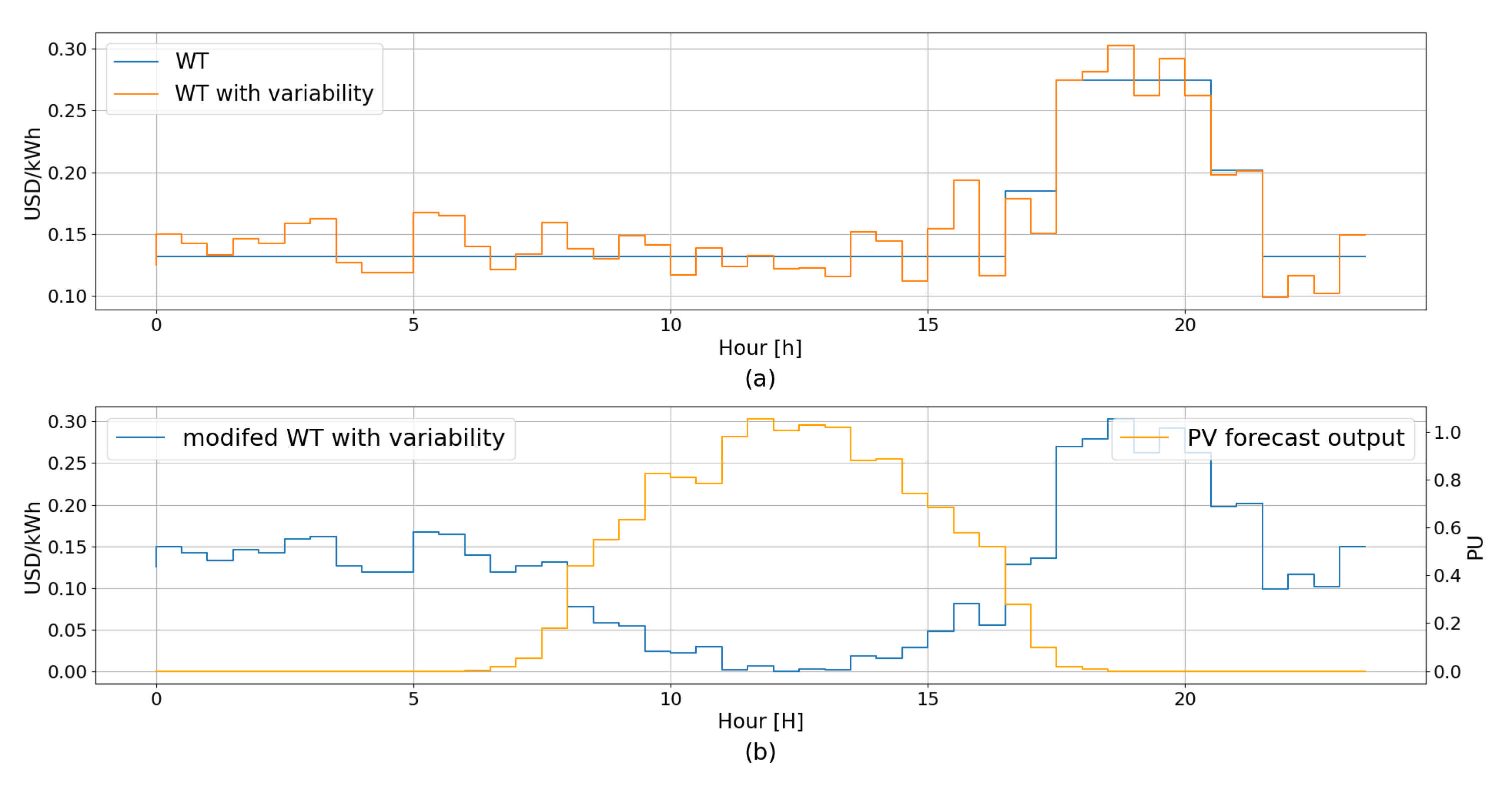
The WT is modified to reflect the PV availability. For more PV output, there is a lower price for the WT in each instant. The original WT, the WT with variability, and the modified variable WT are presented in
Figure 8.
In
Figure 8a, Gaussian noise is added to the WT in order to produce more variability in the WT prices, similar to Real Time Pricing tariffs [
42].
Regarding the EPSO parameters, in all cases, 1000 generations are considered as the stop criteria, and 50 particles per generation.
Figure 9 presents the PV curve utilized and the PV forecast for the next day in per unity (PU) values. The PU curve for the real PV production is based on the PVSS installed at the Federal University of Santa Maria [
43].
The forecast PV output of
Figure 9 is used in the EPSO approach, and the real values are used in the RB strategy.
3.1. EPSO Results
To better visualize the impact of the EPSO approach, for each cluster, the impact of varying the weight w is evaluated, as follows:
comparison of the scheduled demand for w = 1 and w = 0;
Pareto point for the two main parts of the EPSO OF; and
main comparison between the cases with w = 1,w = 0 and the Pareto set.
Table 4 presents the number of requests generated for each cluster. The total number of EVs to be scheduled are 126 for the day-ahead operation; in the
row of the table, the amount of energy in each cluster that has to be supplied is presented. And the
presents the number of all charging modes for each cluster.
Figure 10 presents the scheduled demands for the case with w = 1 and w = 0 for all the seven clusters.
In
Figure 10, for the case with
, the load is more concentrated in the lower periods of the tariff; this behavior is due to the OF of the optimization considering only the cost function
, which in turn reduces the final cost of supplying the load.
For the second case, with w = 0, the load is more distributed, thus filling all the valleys of the first case, which, in this case, ends lowering its PAPR metric, as expected, due to the OF only consider the PAPR part .
To search for a mean term between both functions, according with the modeling, it was defined that the interval for
w is
; thus, after running several simulations, in
Table 5, the Pareto weight find for each cluster is presented.
The found weights for each cluster in the Pareto case are presented in
Table 6.
In
Table 5, when using
the cost function, or
, is minimized, and the PAPR is not taken into consideration. When using
, only
is minimized, and
is now neglected. Finally, the Pareto set for all clusters presents the equilibrium between both metrics.
Figure 11 shows the
metric for all clusters considering
,
and the Pareto set of points.
The cluster with the highest value is C5 that represents the cluster with more EVs to be scheduled.
Figure 12 presents the PAPR values for each cluster and for each case.
In
Figure 12, although the cluster C0 is not the one with highest load demand, the PAPR metric is the one with the highest differences for each of the cases, and, for all clusters, the Pareto point was between
and
.
The Pareto set of points is found based on the values of
and
by changing the
w parameter, and the balance point between them is then selected. As an example, in order to visualize this behavior,
Figure 13 presents the results for the Cluster 5.
As
Figure 13 shows, the Pareto point for EPSO solution was
for Cluster 5, which presents a low impact in PAPR and significant reduction in costs. With these criteria, it is possible to validate the EPSO methodology by comparing it to another MA for the weight found.
3.2. EPSO Validation
In order to validate the heuristic method, the EPSO strategy is here compared to the well known heuristics of Genetic Algorithm (GA) [
7,
9] and Particle Swarm Optimization (PSO) [
37]. As the EPSO is performed in each cluster, the validation of the method is presented here in cluster C5. It should be noted that similar results of performance were found in the other clusters, but here the focus is made on the cluster with the higher number of EVs to be scheduled. It is also considered the weight
w of 0.6 as the one in
Table 6.
The three MA compared consider two stop criteria, the first based on the maximum generations and set to 1000, and the second related to output improvement, where the algorithm stops if there are 15 consecutive generations without improvement. In order to validate the model, all approaches are performed with different population sizes, ranging from 50 to 500. The GA parameters are described as follows [
7,
9].
selection of individuals by Roulette Wheel approach with ;
mutation rate with and ;
crossover rate with .
The PSO parameters are described as follows [
7,
26,
31].
In
Figure 14, the validation outputs are presented for the three metaheuristics approaches in Cluster 5 with
.
Figure 14a–c shows performance of the proposed EPSO compared with GA and PSO. The tests shows that most of the cases EPSO present the fastest results in comparison with GA and PSO. It can be seen that EPSO requires only 3.87 s to obtain a solution with 500 generations, being 80% faster than GA, and 45% faster than PSO. The number of generations to achieve result were less from EPSO methodology requiring only between 15 and 28, which directly impacts simulation time. As can be seen, only for 100 individuals does the EPSO require more generations in comparison with PSO and GA, but, in most of the cases, the EPSO presented a faster convergence.
Comparing OF performance, the EPSO presented better results with the minimal costs, for all of the number of individuals tested. These results prove that EPSO is useful for the proposed framework with a better performance than AG [
18] and PSO [
13,
14] in terms of reduction of speed and improvement of objective function.
3.3. Rule-Based (RB) Impact
RB strategy supports EPSO optimized solution. The required simulation time for RB was 0.0118 s for the total of 48 TSs, which means an average time of 0.246
s for each TS. This very short time for determination of control signals for EVCS makes the RB suitable for application in real time operation, by reducing TSs formulation. The impact in the EVCS, considering
,
, and the Pareto set of points are summarized in
Table 7.
In
Table 7, the three cases are compared. With
, the system presents the best profit for the EVCS, and the EV owner also have a lowered bill price in relation to the other cases. This is mainly because, by using
, the EPSO tends to concentrate the EV load in the lowest periods of the tariff; thus, when the EVCS supplies it with the grid energy, its bill is also lowered.
Although using showed a big difference in the EPSO step, compared to using , in the RB algorithm, the factors, such as the NSCh EV load and the DER’s dispatch, affect the final balance of the system. Nevertheless, the EVCS still presents a better profit when considering only the cost function.
When using , the PAPR is of the system always minimized, and, although this parameter is modified by the NSCh load that has stochastic characteristics, it is still he lower of the three cases.
The Pareto point, in almost all cases, presented a mid-term for every variable of
Table 7.
Figure 15 presents the Pareto demand load in comparison to the tariff.
Figure 16 presents the SCh and the NSCh chargers usage matrix.
Figure 16 presents the chargers usage for the entire day. Vertical values are related to clusters and horizontal values refer to chargers use. The black rectangles are related to the non-commercial hours; thus, is not possible for use by the NSCh users. In addition, the pink rectangles are the available chargers that remain not used because the demand of EV is low. The NSCh requests are being organized, both in the RCH chargers and in the CH chargers, because this type of consumer is advised to use the free SCh chargers whenever possible. It should be noted that, when the SCh chargers are not completely used by all SCh users, the remaining chargers could be used by the NCh users. This is presented in the
Figure 16; for example, the red rectangles at the right side means there are NSCh EVs being recharged by SCh chargers. This behavior ends up creating a left to right movement of the NSC requests. To evaluate the technical impact of the Pareto system in the EVCS,
Figure 17 presents the DERs dispatch for the day-ahead.
In
Figure 17, the BESS is in arbitrage mode, i.e., it is only used in the higher periods of the tariff, providing load supply with a lower base cost, and lowering the grid purchases from the EVCS. The PV output remains serving the load in the generation periods and exports its excess to the BESS whenever is possible.
Figure 18 presents the grid impact considering the EPSO-RB strategy.
In
Figure 18, there is an increase of losses as the EVCS demands energy from the grid. Nevertheless, the losses value are low enough for a high impact to the network, as was set a limit for requirement of energy to the grid. In addition, there are times where the solar generation contributes to sell energy to the network with low losses at hours 15:00 to 17:00.
To evaluate the economic impact of the DERs dispatch in the EV managed load, by using the simple CF system,
Figure 19 presents the relation between the total EV invoice prices and the grid tariff.
In
Figure 19, it can be seen that the Cash Flow (CF) follows, most of the time, the EV invoice, increasing as the EV payments grows. Moreover, the EVCS also profits by selling energy to the grid, as shown in hours 10:00 to 11:00, where there is a low EV invoice but an excess in PV production.
Figure 20 presents the comparison between the CF and the EVCS exchanges with the grid.
In
Figure 20, it is shown that, even when is required energy from the grid, the EVCS presents a positive cash flow by selling energy to the client as presented in hours 3:00 to 7:00 and 19:00 to 21:00. Moreover, in most of the cases, it was not needed to demand high amount of energy from the grid because the DERs supported the EVCS operation.
5. Conclusions
This paper presented a combined framework for day-ahead and real time operation of EVCS. The combined EPSO-RB approach presented fast and good results, and the EPSO algorithm found, for each cluster, the Pareto point of the system when scheduling the requests in less than 4 s for 500 individuals. The RB strategy proved to handle the NSCh consumers demand, thus providing more profit to the EVCS without overloading it. The RB simulation time were less than 0.3 s.
Although the best profitable scenario found was with only the cost function taken into account, as the EVCS belongs to the Grid Utility, it is also important to reduce the peak of the system to avoid overloading whenever using the grid for energy exchanges. Thus, the Pareto approach also presented an efficient method to find a mid-term between the economic and the technical metrics. Finally, the RB strategies presented high flexibility by handling the NSCh loads given the stochastic characteristics of both the EVs and the PV.
As this methodology presents a flexible option to handle real-time problems and provides more profit to the EVCS, this approach is considered to be implemented in large electric cars electrovias, as the one in Reference [
21]. For this purpose, the methodology would require some changes, such as lower TSs, which can be easily implemented. In addition, the real-time RB strategy could be crucial to the EVCS given the lack of practical data on EVs charging behaviors. Moreover, the system is able to combine both optimized decision-making provided by the scheduling and also to handle real-time EV demand. Finally, as the scripts were developed in a open source language, it is easier to have interoperability with Raspberry micro controllers in practical applications.


 ,
, 


