1. Introduction
Drilling automation has become an important topic after many years of slow adoption. Yet, the automation of the drilling process can be addressed at very different levels. Macpherson et al. (2013) [
1] have defined ten levels of automation (LOA), starting with being completely manual at level 1 and reaching full automation at level 10. At the highest LOA, all the monitoring, generating, selecting, and implementing functions are performed by a computer system. In other words, the drilling system can be considered as completely autonomous. The major difference between automation and autonomy is that the first one refers to the ability to control a system while the latter shall, in addition to control, be able to respond to unexpected situations.
Some of the first ideas for applying automation to the drilling process date to 2004 [
2]. It became clear that executing automated procedures could not be done without several protection mechanisms such as safe operating envelopes (SOE) and fault detection and mitigation (FDM) [
3,
4]. The application of standardized procedures under the protection of SOE and FDM functions have shown that automated drilling operations were both possible [
5] and increased the efficiency [
6]. Attempts have been made to integrate downhole measurements from high-speed telemetry in a closed loop control architecture [
7,
8]. Also, the control of drilling parameters has been automated using closed loop control [
9,
10].
With the advent of several drilling automation solutions that require access to the drilling control system (DCS), open interfaces have been developed [
11] and new software architectures for the DCS have been designed [
12].
Automation has also started to be applied to directional drilling when utilizing rotary steerable systems (RSS) [
13], but also with positive displacement motors (PDM) by solving the decision-making problem of when to slide or rotate to achieve a trajectory with as little tortuosity as possible [
14,
15]. Those considerations for when to rotate or slide in directional drilling are borderline with autonomous control considerations as they relate to automatic decision-making in addition to control considerations. Yet, to the best of our knowledge, autonomous decision-making and control of the drilling process has not yet been addressed.
There are two paths to achieve fully autonomous drilling: either rely on the presence of a human operator in case the autonomous system is unable to recover from an unexpected situation or design the system from scratch to never need any human assistance of any form. The second alternative may be mandatory for very constrained environments such as space exploration missions where distances and communication delays render human interventions impractical or impossible, however in the context of drilling operations, it is always possible to rely on the presence of a human operator and therefore the solution described in this paper is based on the availability of a fallback “pilot” (the driller).
The research question addressed in this paper is the following: can we achieve safe and efficient autonomous drilling, considering that a human operator can intervene in case automatic recovery fails?
2. Problem Scope
Despite the very general nature of this research question, we have chosen to limit the scope of work. First, by drilling we only consider the conditions for which the drill bit can go on bottom without requiring to make a drill pipe connection. In practice, this constraint implies that we do not consider tripping, reaming, and back-reaming operations. Second, we limit ourselves to conditions for which the annulus is not closed and where a single fluid is used. Because of this second constraint, we do not address underbalanced, managed pressure, dual gradient drilling operations, or well control situations. Third, we only consider drilling performance, therefore excluding questions related to wellbore positioning, geo-steering, cementing, formation strength evaluation, e.g., leak-off test, etc. Fourth, the automation of pipe handling is out of our scope because it can be seen as an independent task with regards to the drilling process management and therefore can be treated separately. The proposed solution should nevertheless be valid for:
Land rigs, fixed platforms, or floaters;
Any depth ranges and well shapes;
Simple or tapered drill-strings and wellbore architectures;
Under-reaming or hole opening operations;
Water-based, oil-based, or synthetic-based drilling fluids, but not foams as this would lead to a dual gradient drilling operation;
Complex hydraulic networks with multiple paths such as leakage to the annulus from an under-reamer, hole opener or positive displacement motor, or the use of booster pumping in a riser;
Low and high bandwidth communication methods, including possibly distributed sensors along the drill-string.
As the problem of autonomous drilling is about taking decisions when confronted with deviations from the planned drilling operation, those choices have a direct impact on the overall drilling performance and the possible occurrence of drilling incidents. Indeed, a multitude of different drilling hazards may occur during a drilling operation. Typical ones are formation fluid influx, formation fracturing, hole collapse, stuck-pipe, pack-off, formation washout, failure of downhole components, breakdown of drilling equipment, etc. On the one hand, the sequence of actions decided by an autonomous drilling system shall avoid, if possible, to lead to any of those situations. On the other hand, it is important to maintain a good overall performance for the drilling operation. Drilling too fast can lead to drilling incidents, for instance associated with inefficient cuttings transport, but drilling too slowly may also end up with other sorts of drilling incidents for example associated with wellbore instabilities as the open hole formations are left unprotected for too long.
Each decision taken during the drilling process shall be evaluated in the perspective of multiple time horizons. The decision shall not cause an immediate increase of the risk level, and at the same time it shall help control the risk levels in the medium term and minimize the overall duration of the drilling operation for the long term. We consider in our approach both data-driven techniques and physics-based models, the result being a hybrid artificial intelligence system. Visualization of the internal state of the system is actively used as an attempt to convey the details behind the decisions taken by the algorithms and thus provide insightful information about the decisions taken by the system (for more details on these and other features that are relevant for the models’ interpretability see the thorough analysis in [
16]).
Because of the criticality of the domain and problem, it is crucial that the autonomous drilling solution is robust with respect to the uncertainty embedded in the process and possible incidents that may occur, such that the users can build up trust in the system. Hence, the proposed solution includes implementation of several protection layers that ensure safe behavior both in case of failures and commands that violate the limits of either the machines or the process. In the eventuality of a drilling incident, remedial actions need to be taken. These actions cause delays and the overall duration needed to reach the section total depth (TD) increases. Therefore, if we are capable to estimate the probability of occurrence of drilling incidents as well as the delay they can cause if they occur, it is possible to estimate their impact on the drilling time. So, a way to solve the autonomous drilling problem is to find a series of actions that is capable of minimizing the time to reach the section TD. This duration is decomposed into two parts:
More formally, this can be expressed as:
where
is the estimated time to reach TD,
is a series of actions
,
is a function that estimates the duration that will take to execute an action,
is a possible drilling event chosen from a set of possible drilling events
,
is the occurrence probability of a drilling event
, and
is the estimated duration required to mitigate a drilling event.
If a series of actions is too aggressive and therefore increases the risk of occurrence of drilling incidents, the result may be a longer delay in reaching the section TD than with a series of actions that does not raise the risk level and yet maintains a good performance level. The problem at hand is therefore to find the series of actions that minimizes the estimated duration to reach the section TD, i.e., to solve the following equation:
where
is the set of all possible series of actions to reach the section TD.
This minimization problem is estimated from the current physical state of the drilling system. As the drilling system is observed only very sparsely, both in space and time, the physical drilling system state is known with a degree of uncertainty.
3. State Estimation and Uncertainty
In physics, state variables are the variables that describe the mathematical state of a dynamic (time-dependent) system. A physical system is usually described by a set of partial differential equations where the variables are physical quantities such as time, position, velocity, volume, tension, stress, strain, temperature, pressure, etc., which describes how certain physical quantities like mass, momentum, and energy are conserved. The drilling system contains three sorts of components that can have motion relative to each other: the drilling fluid, the drill-string, and entrained particles/bubbles immersed in the drilling fluid. The drilling process is therefore described by applying conservation laws to these three component types:
Mass conservation for the drilling fluid [
17]:
, where
is the drilling fluid density,
is time,
is a fluid velocity vector;
Momentum conservation for viscous flow (Navier-Stokes) [
17]:
, where
is pressure,
is the stress tensor,
is the gravitational acceleration and
represents external body force;
Force balance on particles/bubbles transported by the fluid (Newton) [
18,
19]:
, where
is the density of the background fluid,
is the particle volume,
is the particle velocity vector,
is the external force vector applying on the particle;
Torque balance on particles/bubbles transported by the fluid (Newton): , where is the particle density, is the angular velocity of the particle, is the second moment of area and is an external torque applying on the particle;
Energy conservation for heat transfer (Fourier) [
20]:
, where
is the enthalpy per mass unit,
is the forced convective term,
is the conductive and natural-convective term,
is the heat generated by mechanical and hydraulic frictions. The enthalpy can be expressed as a function of temperature
and pressure by the following expression:
, where
is the specific heat capacity,
is the volume, and
is the volumetric coefficient of thermal expansion;
Force balance for elastic deformation of the drill-string (Newton) [
21]:
, where
is the internal tension vector in the solid,
is a curvilinear abscissa,
is an external force per unit length,
is the density of solid constituting the string,
is an area and
is the velocity of control element of a portion of string;
Torque balance for elastic deformation of the drill-string (Newton) [
21]:
, where
is the internal torque in the solid,
is the tangential vector of the Frenet–Serret coordinate system,
is an external torque,
is the second moment of area, and
is the angular velocity of a control element of a portion of a string;
Energy conservation for linear deformation of the drill-string (Euler-Bernoulli) [
22]:
, where
is a deflection in a perpendicular direction to
,
is the elastic modulus,
is a mass per unit length, and
is the potential energy of external loads.
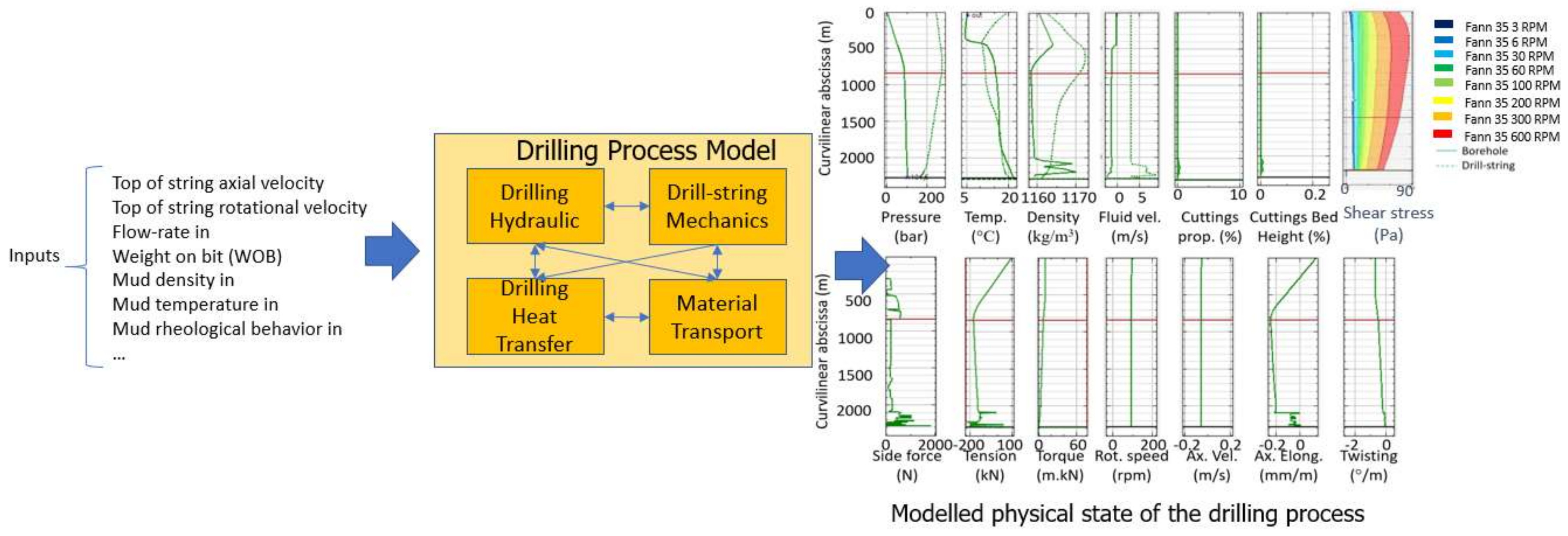
The resolution of these partial differential equations describes fully the time evolution of the physical drilling system state in terms of the following variables:
,
,
,
,
,
,
,
,
,
, and
. This resolution depends on the boundary conditions that are imposed by the drilling machines, i.e., top of string position, axial and rotational velocities, volumetric flowrates, and on- or off-bottom condition (see
Figure 1).
These partial differential equations, except for the mass conservation, depend on external contributions, i.e., ,, , , , , and . Some of these contributions can be directly estimated, like for instance the effects due to gravitation, buoyancy, viscosity, when the physical properties of the system components are known, e.g., geometrical dimensions, density, compressibility, thermal expansion, rheological behavior, specific heat capacity, thermal conductivity, Young’s modulus, Poisson’s ratio.
However, some other external contributions may depend on the information that is not readily available as for instance the formation rock unconfined compressive strength and angle of internal friction when evaluating rate of penetration (ROP). These values change as new rock layers are drilled and therefore need to be constantly calibrated.
That is also the case of static and kinetic mechanical friction factors between the drill-string and the borehole. These properties are used to estimate the mechanical friction forces and torques [
24]:
where
is the total kinetic friction force vector,
is the upper limit of the static friction force,
is the limit of the kinetic friction force at high velocity,
is the slip velocity between the two surfaces, and
is the critical Stribeck velocity. In addition, the static and kinetic friction limits are expressed as:
where
and
are respectively the kinetic and static coefficients of friction,
is the reaction force between the surfaces in contact, and
is the normal unit vector at the contact. The calibration of the coefficients of friction is typically made during conditions where the bit is off bottom, like for instance during a pick-up or a slack-off sequence, or when rotating off-bottom [
22]. For boundary friction, the coefficient of friction is mostly influenced by the viscous properties of the fluid, and therefore as long as the drilling fluid characteristics do not change, the coefficients of friction should stay relatively constant. This being said, when picking up or slacking-off the drill-string, tool-joints may be dragged into a cuttings bed therefore causing additional forces on the tool-joints that were not necessarily accounted for by the model. In such a condition, when calibrating the mechanical friction based on pick-up and slack-off motions of the drill-string, the apparent mechanical friction will probably increase. However, when rotating off-bottom, the calibration of the mechanical friction may give a different result than when utilizing drag forces, because the unaccounted torque generated by rotating the tool-joints in the cuttings bed does not necessarily result in a torque of a similar magnitude as the apparent increase of mechanical friction caused by drag forces. It is therefore convenient to distinguish the coefficients of friction,
,
, which are only associated with mechanical friction, from friction factors that correspond to apparent coefficients of friction for the total effect of various forces and torques that are not only limited to mechanical friction but not accounted by the model [
25]. It turns out that the apparent axial and rotational friction factors may differ because the subjacent unaccounted forces and torques are of a different nature. We will denote
and
the respective sliding and rotational friction factors (dimensionless). Another example of additional forces and torques that may influence the magnitude of
and
is related to differential sticking forces resulting from a thick mud cake after drilling a highly porous and permeable formation layer.
Even some of the contributions that should be simple to evaluate may be difficult to assert because of missing information. For instance, the effect of gravitation and buoyancy on a cutting particle is difficult to estimate simply because the volume and density of an individual cutting particle is not known. This uncertainty can influence hydrostatic pressure calculations, cuttings transport [
26], viscous pressure losses and even drill-string torque through the grinding mechanism that takes place when cuttings are trapped between a tool-joint and the borehole [
27]. Also, the wellbore size may be different from the theoretical one. This can be caused by hole collapse, formation washout, i.e., hole enlargement, but also because of accumulation of debris, e.g., cavings or cuttings therefore resulting in borehole constrictions. So, in a similar way to friction factors used for accounting for ill-defined effects on mechanical forces and torques, it is possible to utilize an annulus hydraulic friction factor,
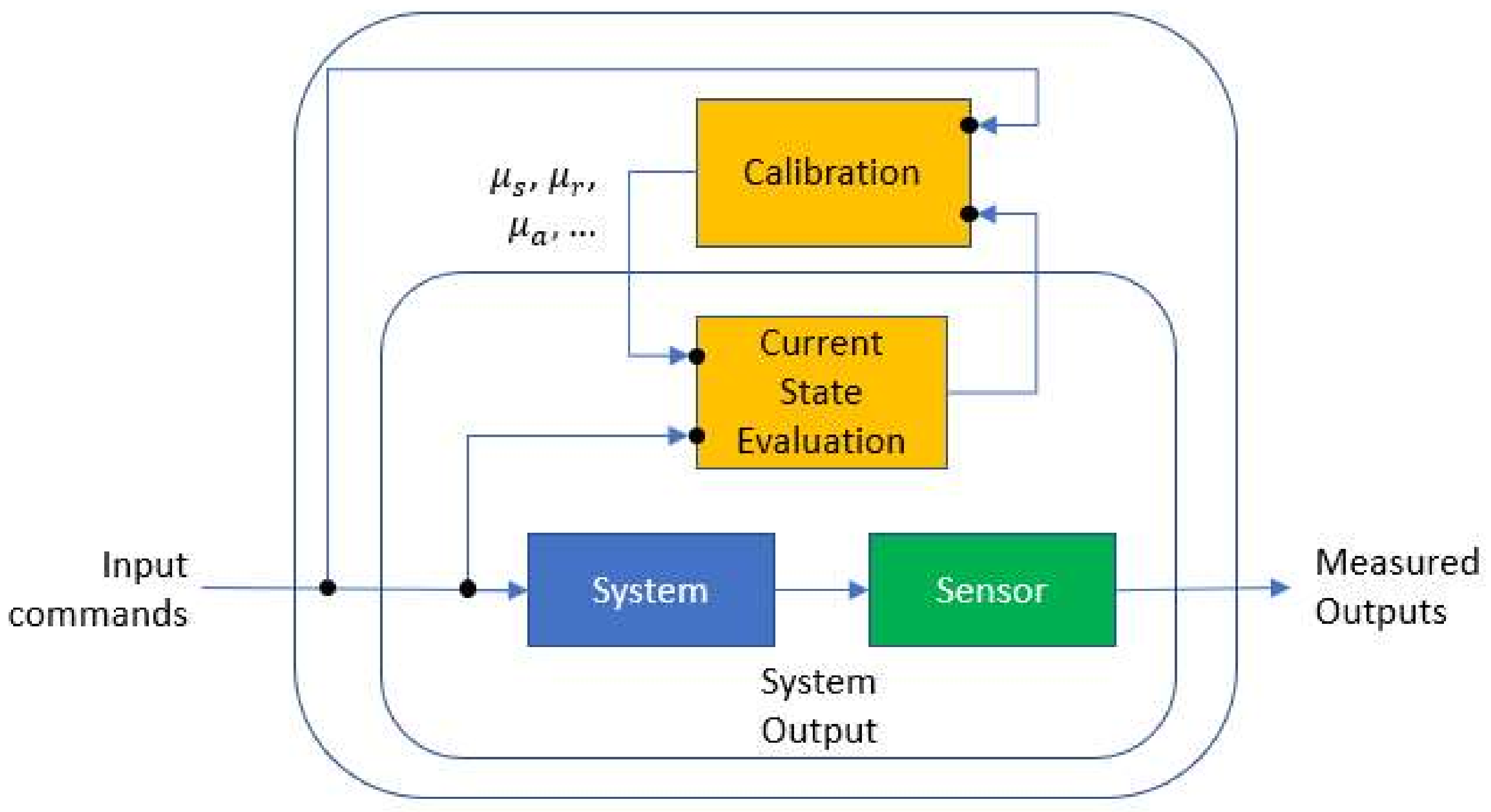
(dimensionless). In perfect conditions, this correction factor should be equal to one, but if it increases this may indicate that additional pressure losses arise from an obstruction and if it gets smaller that may be a sign that the borehole is larger than expected (see
Figure 2).
4. Protection Layers
To ensure safe drilling operations, an autonomous drilling system shall embed mechanisms that are capable of automatically protecting the drilling process. We propose three levels of protection:
Protection of the commands sent to the drilling machines, also referred to as safe operating envelopes,
Protection of the drilling process, i.e., automatic fault detection, mitigation, and recovery (FDMR);
Protection of the process during transition from autonomous to manual control by automatic management of safe operational modes.
The purpose of the safe operating envelopes is to ensure that no set-points can be sent to the drilling machines that can lead directly or indirectly to a drilling incident. Here, we suppose that similar safe envelopes exist to protect the drilling machines but that they are implemented directly in the drilling control system (see
Figure 3).
The role of FDMRs is to automatically detect abnormal drilling situations and to react accordingly. As a first response to a drilling incident, actions are taken to mitigate the problem and as a subsequent set of actions, remedial procedures are engaged to cure the problem and return to normal drilling conditions.
Safe modes management is ensured by automatic procedures that will be triggered in case of failures. These procedures will put the drilling system in a state that should not immediately cause a worsening of the drilling conditions. This is to allow a driller to regain manual control of the drilling operation in a safe manner, even though his situation awareness may be very low while the autonomous drilling system is in control.
4.1. Safe Operating Envelopes
During drilling, it is important that the set-points sent to the machines are within certain limits that ensure safety of the process. These limits are given by the safe operating envelopes which are continuously computed by the underlying algorithms [
28]. The safe operating envelopes provide protection limits for the three control parameters relevant for drilling, namely mud-pumps setpoints, top drive setpoints, and draw-work setpoints. We will now succinctly describe three of those (for more detailed information see [
23]):
4.1.1. Axial Velocity
When it comes to drill-string axial velocity, the system continuously computes which are the maximum allowed limits, depending on the downhole conditions and if the setpoints provided are not within these limits, then the system will oversteer the setpoints with own predefined values. This is to ensure that the axial velocity, which has a direct impact on the velocity profile of the drilling fluid, should not introduce additional pressure loss or gain which can trigger instability in the downhole conditions, namely swab or surge. For instance, an upward movement of the drill-string will induce a decrease in the downhole pressure which should not be below the pore pressure or the collapse pressure of the open hole formations. Similarly, a downward movement of the drill-string will have a mirrored effect. The computation of the safe operating limits for the axial movement is adaptive to the current system state:
If there is no circulation, the limits are computed as a function of the gel duration.
If there is circulation, the limits are computed as a function of the drill-string rotational speed and flowrate.
4.1.2. Flowrate
The pressure in the open hole wellbore should stay within the pore- and fracture pressure margins of the formation to avoid influx of reservoir fluids or fracturing the well. The flowrate of the fluid pumped in the wellbore will influence the pressure, and there is a maximum flowrate that ensures not fracturing the open hole formation. The maximum flowrate depends on the operational variables and downhole conditions such as:
Drill-string axial velocity and heave levels;
Drill-string rotational velocity;
Bit and bottom hole depths;
Temperatures;
Cuttings load.
The system continuously calculates the maximum allowable flowrate which keeps the pressure safe below the fracture pressure for the current operational variables and downhole conditions. If the driller or the automated drilling system requests a flowrate set-point that is above the maximum allowable flowrate, the flowrate set-point to the mud pump controller is reduced to the maximum flowrate to ensure a safe operation.
If the well has been left without circulation for a while, for example during a pipe connection, the gel strength of the drilling fluid has increased. The gel strength is an important property of the drilling fluid since it keeps the drilled cuttings in suspension when circulation is stopped, but care must be taken when starting up the pumps to avoid large fluctuations in the annulus pressure when breaking the gel. To keep the well safe during pump start-up, the system will calculate a minimum waiting time for establishing circulation after the first flowrate change to avoid risking a high surge of pressure that a new pump acceleration could cause.
High pump acceleration can also cause pressure spikes in the annulus, resulting in well fracturing. In addition, it can be difficult to distinguish large pressure variations caused by high pump accelerations from pressure variations caused by pack-off. Large pump decelerations can generate a swab pressure that can cause influx of formation fluids. The system continuously calculates maximum pump accelerations and decelerations to avoid well fracturing or formation fluid influx. The calculation considers the bit and well depth, temperatures, and cuttings load.
4.1.3. ROP
The adaptive ROP management is aimed at local drilling performance optimization, taking into account short-term effects (as opposed to the long-term effects considered by the decision-making in the autonomous drilling modules). The optimization task entails finding parameter set-points for the mud pump, top drive, and draw-works such that the resulting ROP is maximized while avoiding potential drilling incidents, which are treated as constraints for the optimization problem.
The system uses a bit-rock interaction model that estimates ROP as a function of weight on bit (WOB), top-drive speed, and mud pump flowrate, while taking into account the cutting and friction processes underlying the bit-rock interaction. It is based on the model of Detournay et al. (2008) [
29] which provides steady-state relations between WOB, torque on bit, and depth of cut per revolution, coupled through a series of formation and bit-related parameters. The model describes three separate phases of the bit response: a first phase where ROP is less reactive to changes in WOB, a second phase where a sharp increase of ROP is observed with additional WOB, and a third phase where ROP stagnates or even decreases as more WOB is added. The transition between phase 2 and 3 corresponds to the “founder point.” A linear variation of ROP with WOB is assumed in all three phases in our implementation of the model. The detailed equations can be found in [
30,
31].
The ROP model needs to be continuously calibrated as drilling advances, since the formation and bit properties may change, either suddenly, as in the case of drilling through a hard-stringer, or gradually, for instance due to bit wear. The following parameters require calibration:
Formation unconfined compressive strength (UCS);
Formation angle of internal friction;
A parameter related to the cutting forces orientation (proxy for bit aggressiveness);
Threshold for transition between phase 1 and 2 of the bit response;
Threshold for transition between phase 2 and 3 of the bit response (founder point);
Two parameters related to the variation of frictional force with WOB in phase 1 and 3, respectively. The latter influences the stagnation or decrease in ROP as WOB is added beyond the founder point.
The calibration uses a Sequential Monte Carlo (particle filtering) method [
32], which takes measurements from surface sensors (WOB derived from hook-load, ROP, top-drive torque and rotary speed) and evaluates many different model realizations (“particles”) generated using a stochastic process (e.g., random walk). All particles, and their corresponding formation and bit parameters, are weighted based on the match with the measured WOB, torque, and ROP values, at a given time step. This results in probability distributions for all the calibrated parameters, which can be summarized using their means and variances, and further propagated to the other modules of the ROP management system. Further details of the particle filter implementation can be found in [
30].
Next, the drilling constraint module continuously evaluates various combinations of drilling parameters with respect to the following incidents:
Onset of drill-string sinusoidal buckling;
Poor cuttings transport, leading to formation of cuttings beds;
Excessive cuttings concentration in suspension, leading to pack-offs;
Exceeding of geo-pressure margins, defined by the pore, collapse, and fracture pressure, and minimum horizontal stress;
Excessive mud-pump pressure.
The computations above are based on steady-state drilling models, consisting of hydraulics, heat transfer, cuttings transport, torque and drag, and buckling models. These models have been described in detail in previous publications [
20,
26,
33,
34]. Each model is updated in real-time at frequencies ranging from 1Hz to 5Hz, which ensures the adaptive nature of the drilling constraints computations. The ROP is evaluated for a given combination of drilling parameters using the calibrated bit-rock interaction model described in the previous section. The system checks that these parameter combinations lie within the safe ranges defined by the drilling constraints, such that they maximize the ROP computed by the bit-rock interaction model at a given time. In addition to the drilling constraints described above, the set-point generation process includes limits on the incremental change of drilling parameters, and only allows one parameter to be changed at a time.
The optimum set-points are found using successive grid searches over the individual ranges of the three main variables—WOB, top drive RPM, and mud pump flow rate—with maximum increments defined by , respectively. The drilling parameters can be either increased or decreased by these pre-configured amounts. If a valid new set-point is not found by changing one parameter at a time, the algorithm allows several parameters to change simultaneously. If this still does not lead to a valid solution, it increases the search increments , and repeats the entire process with the increased search space.
4.2. Fault Detection, Mitigation and Recovery
4.2.1. Overpull/Set-Down Weight
The system needs to react fast to abnormal drilling variables such as excessive hook load, torque, or pressures to avoid ending up with serious drilling problems like stuck pipe or well fracture. The drilling automation system continuously calculates maximum and minimum values for hook load, torque, and pump pressure, accounting for changing drilling conditions such as bit depth, temperatures, and cutting concentrations in the wellbore. In our case, the implemented approach for calculation of maximum and minimum values is model-based, using the observer-based approach described in [
4]. The drilling control system is continuously updated with the maximum and minimum values for hook load, torque, and pump pressure. If some of the values are exceeded, a set of actions is carried out to mitigate and recover from the fault.
In case the hook load exceeds the maximum or minimum values, the immediate reaction is to move the drill string in the opposite direction to avoid that the pipe gets stuck, or experiences excessive buckling. There may be stretch or buckling in the drill string, and especially in long wells it may take some time before the bit starts to move when pulling or lowering the pipe. When the top of string has moved a distance (calculated by the system) sufficient to get the bit in motion, the movement is stopped. In an autonomous drilling system, the system also needs to recover from the fault to be able to continue the drilling operation. Excessive overpull or set-down weight may be caused by an obstruction in the annulus which prevents the drill string to move, such as a cuttings bed. The recovery procedure is therefore to reciprocate (move drill string while pumping and rotating) to try to clean the hole. If the reciprocation is performed without any erratic hook load or torque, the drilling operation can continue. If the reciprocation cannot be carried out without erratic or excessive hook loads, the system is set in a safe mode.
4.2.2. Over-Torque
In case of an over-torque, the first reaction is to stop the rotation, unwind the torque, and lift off the bottom, to avoid pipe twist-off or stuck pipe. The first step in the recovery procedure is to move the drill string up/down without rotation. If this is completed without any erratic or excessive hook loads, the system tries to start drill string rotation stepwise. The final step in the recovery procedure is to reciprocate until the drill string moves without any erratic torque or hook load.
4.2.3. Overpressure
Pack-offs are typical drilling incidents that may occur during a drilling operation. To detect a bridging or pack-off situation, the system compares the measured pressures along the hydraulic circuit with estimated ones. Ideally, the position of these pressures should be along the annulus, yet as most drilling operations rely on mud pulse telemetry, it would be too uncertain that the detection would take place in a timely fashion if it were based on measured downhole annulus pressure transmitted by such a low bandwidth communication medium. Unless high-speed telemetry is available, the standpipe pressure (SPP) is used as an overpressure detection point, even though the detection could react to obstructions occurring inside the drill-string and which would be harmless for the open hole formations. If an overpressure is detected, a mitigation procedure is initiated. The mud pump rate is immediately reduced to a predefined value in order to observe how the drilling system responds to these step changes. Also, if the drill-string is on bottom, it is lifted over a minimum distance that ensures that no more cuttings are produced. After observing the response of the drilling system to the step change in flowrate, either it is evaluated that the obstruction is incompatible with any circulation and the mud pumps are stopped, or a new flowrate is estimated that would allow to circulate without risking causing an excessive annulus pressure below the flow restriction. The procedure may be repeated several times if the flow conditions continue to deteriorate [
3]. If stabilization of the flow conditions is achieved, then the system starts a recovery procedure. To attempt recovering from the bridging situation, the system starts reciprocating the drill-string in order to erode the accumulation of debris that initially caused the overpressure situation [
28].
4.2.4. Drilling Dysfunctions
The ROP management system can operate in both WOB and ROP control modes. While the set-point generation described in
Section 4.1.3 works internally with WOB as a control variable, the resultant ROP set-point (computed from the calibrated bit-rock interaction model) can be fed to the control system instead. When using the ROP control mode, the system monitors the WOB to ensure that it does not exceed a maximum WOB threshold reflecting uncertainty in the bit-rock interaction (e.g., when drilling into a hard stringer, or when drilling above the founder point). If this WOB threshold is exceeded, the system automatically switches to WOB control mode with a set-point defined by the maximum WOB.
In the case of exceeding the founder point, the current estimate of the bit-rock interaction remains valid, and only the founder point parameter needs to be adjusted. As such, the system will gradually increase ROP while staying below the updated founder point. On the other hand, when drilling a hard stringer, the system will initially be in a state where the bit-rock interaction parameters are no longer valid, and the system will automatically adjust its parameters, in particular the UCS, which will be then used to compute a reduced ROP set-point.
It should be noted that the system presented in this paper currently does not consider detection and mitigation of drill-string vibrations, but these shall be included in future work.
4.3. Safe Mode Management
In the context of both automated and autonomous systems, the situation awareness of the driller is highly decreased [
35]. Hence, in abnormal situations where the control needs to be switched from the autonomous or automated to manual mode, it is crucial that the system is left into a state that ensures safe process for a certain amount of time. This is necessary to allow the driller to regain control of the machines in a manner that does not trigger unnecessary deterioration of the downhole conditions.
In the present context of autonomous decision-making, the internal state of the system needs to be continuously monitored and, any deviation from normal behavior should immediately be handled. Failures in communication or failures in the hardware equipment can arise and, these are typical triggers that will influence the internal state of the system and consequently the autonomous decision-making capabilities. The management of the transition from autonomous to manual control, which is an integral part of the overall system, ensures responsible and safe behavior of the artificial intelligence (AI) system (for more detailed information on this, see [
36]).
An automated response in case of hardware failures or unsuccessful recovery is ensured by two main modules, as illustrated in
Figure 4. The first module monitors continuously the state of the process and keeps track of the current context, while the second module decides the context-specific actions that should be performed if failures occur. Hence, this approach ensures robustness of the system and a safe process in case of failures and, consequently a smooth transition from autonomous to manual control.
5. Drilling Procedures
Under the protection of the safe operating envelopes, FDMRs and safe mode management, it is possible to execute series of drilling commands that are sent to the drilling machines. Such a series of machine set points is a typical drilling procedure. A drilling procedure can be seen as a recipe, i.e., a sequence of instructions. The International Society of Automation (ISA) defines a standard (ISA-88 [
37]) that makes use of the concept of recipe. ISA-88 is a method to analyze batch control. The meaning and scope of batch control is for any manufacturing process that produces more than just a few products, also referred to as job production, but less than a mass production process, sometimes denoted as flow production. In such a context, a batch is a limited quantity of something. Indeed, one can see the drilling of a well section as a batch, since we need to drill a well-defined number of stands in order to reach the section TD. Furthermore, the concept of batch drilling has also been adopted for some field developments where all identical well sections are drilled in one batch [
38]. ISA-88 describes a batch process using three models:
A process model: it is a hierarchical decomposition of the overall process into process stages, which are themselves subdivided into process operations, which make use of the process actions.
A physical model: it is also a hierarchical categorization of the overall enterprise, into sites which consist of areas, themselves containing process cells, in which there may be units, themselves composed of equipment modules, which finally may be made of control modules.
A procedural control model: it describes how the batch process should be carried out. It is also hierarchically organized with the first level subcategory being a unit procedure, the second hierarchical level being an operation, which itself is made of phases.
The ISA-88 standard provides a way to structure batch process control in a hierarchical way. For instance, at a high-level point of view, a procedure, i.e., from the procedural control model, in combination with process cells, i.e., from the physical model, carries out a process, i.e., from the process model perspective. Also, ISA-88 defines methods to deal with exception handling.
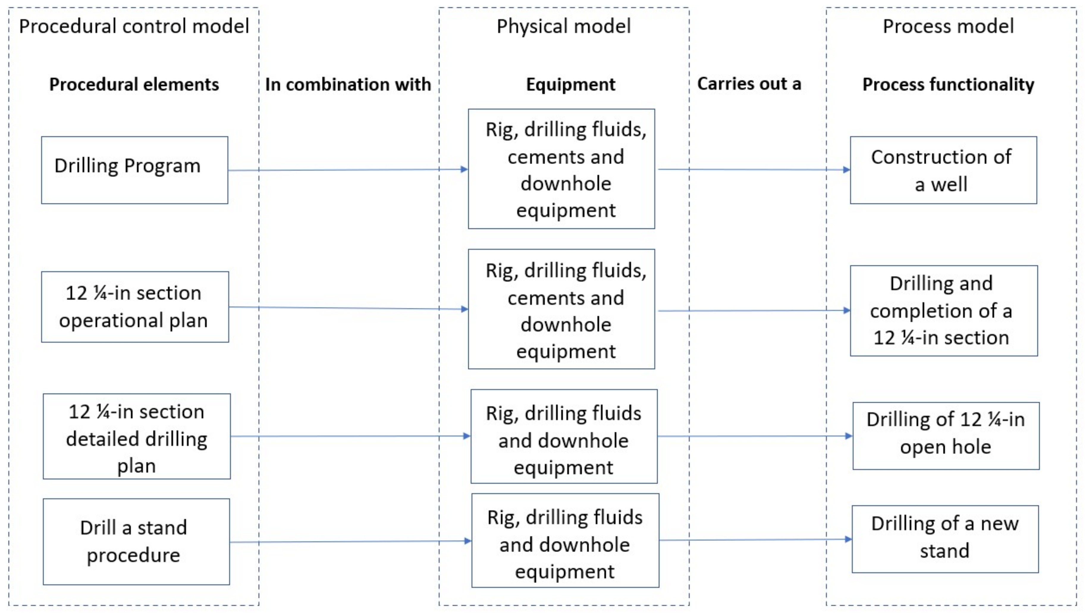
Figure 5 shows a possible decomposition of a drilling operation utilizing the ISA-88 method. For the higher levels of abstractions, the ISA-88 standard suits well with the well construction process and offers a structured way to analyze the drilling process. However, at lower level of detail than drill or trip a stand, the standard falls short to address the complexity of an actual drilling operation. This is because there are not just a few possible recipes that can apply at any time, but multiple variations that need to be chosen as a function of the current situation. At that level of detail, the drilling process is not a batch process, instead it is job production, i.e., closer to handcrafting than to plant manufacturing. For instance, when drilling every single stand, the driller shall decide whether he should stage the mud pumps several times or reach the nominal speed in one step after breaking the gel. The decision for the one or the other could depend on the possible risk for pack-offs. He should also decide whether he shall start the top-drive while establishing circulation, maybe to assist in breaking the gel or because there is a risk of differential sticking, while the action may require that he needs to stop the top-drive afterward to take a survey. He may have to decide whether it is necessary to lift off bottom while drilling the stand because of pack-off tendencies or heavy drill-string vibrations. He may have to decide whether a reciprocation is needed after drilling the stand, for instance, if the ROP was very high and there is a risk that cuttings may pack around the BHA when establishing circulation after a connection. Or he may decide to take a friction test in order to check whether there are accumulations of cuttings along the borehole.
Even though there are multiple choices that shall be decided when drilling every single stand, it is still useful to proceed with several levels of abstractions in order to not be overwhelmed by the unnecessary complexity. For instance, when starting the mud pumps, there are detailed choices that should be made:
Should we use two out of three mud pumps so that the third one can be used as a booster pump to clean the marine risers?
Should the mud pumps be started with different pump rates in order to minimize the risk of accentuated stroke noise that can perturb the decoding of mud pulses from downhole telemetry?
For that reason, it is useful to decompose the problem into different levels of abstractions. Here, we will use the terminology of the Zachman framework [
39], where the levels of abstractions are, from high to low:
Contextual level, i.e., drilling a 12 ¼-in section,
Conceptual level, i.e., drilling one stand,
Logical level, i.e., running a friction test,
Physical and detailed level, i.e., unwinding the drill-string to reach zero torque after stopping the top-drive.
The contextual and conceptual levels are already addressed through ISA-88, therefore we will focus on the logical and physical levels.
5.1. Logical Level
At the logical level, drilling a stand can be decomposed into a series of procedural operations (utilizing the ISA-88 terminology) (see Figure 5 in [
36]):
Take off slips: when the drill-string is in slips, it is lifted to transfer the weight from the slips to the top-drive.
Top-drive startup: the top-drive may be ramped up in one or several stages. The accelerations and stages should be chosen carefully to limit the risk for intense drill-string vibrations, at least in deviated wells.
Mud pump startup: first the air gap at the top of the drill-string needs to be filled without using too much time. Then circulation must be established. This means breaking the gel and reaching a steady flow into the whole hydraulic circuit. Breaking the gel may be assisted by rotating the drill-string. Then the mud pump rate is increased toward its nominal value. This can be done in one or several steps depending on the operational risks for pack-offs or differential sticking. It may be necessary to stop the top-drive, if it was running, and a survey shall be taken. If the top-drive has been stopped, it may be necessary to lift up and down the drill-string several times in order to remove some of the trapped torque, at least for deviated wells. When mud pulse telemetry has been established, the top-drive may be started.
Tag bottom: on a floater, the heave compensator may need to be started. Furthermore, the axial tagging velocity shall be chosen to give a clear signal that the bit is on bottom and yet not be the source of large stick-slips because of a large step-change in WOB when touching the bottom hole.
Drill: the drilling parameters, i.e., WOB, top-drive speed, and flowrate, should be continuously adapted to the current drilling conditions both to optimize the penetration rate but also control risks of drill-string vibrations and poor cuttings transport.
Reciprocate: to improve the hole conditions it may be necessary to ream-up and down for a certain distance. The choice of top-drive speeds, axial velocities, and flowrates should be adapted to the current downhole conditions and potential risks for pack-offs and surging.
Perform a friction test: if information about the downhole mechanical friction is necessary, a pick-up and a slack-off procedure may be performed. The pick-up distance and the axial velocities should be chosen as a function of the length of the drill-string, expected friction, and possible consequences on swab and surge pressures. The flowrate may also have to be adjusted for performing the friction test.
Move to stick-up height: on a floater it may be necessary to stop the heave compensator if it was turned on. Then the drill-string is lowered such that the tool-joint is at the correct level for the iron roughneck.
Stop top-drive: the top-drive rotation speed is brought down to zero with a controlled deceleration. With deviated wells or if heave variations are low, it may be necessary to apply a zero-torque procedure consisting of unwinding the drill-string to remove the torque that is still trapped in the drill-string because of the mechanical friction.
Stop mud pumps: the mud pumps are ramped down with a controlled deceleration procedure in order to avoid large downhole pressure variations due to the drilling fluid inertia effects.
Set in slips: the slips are closed, and the drill-string is lowered to transfer the weight from the top-drive to the slips.
Perform booster pumping: during any procedural operations where the mud pumps are active, it may be necessary to pump from the bottom of the riser in order to assist lifting cuttings that are trapped in the riser.
5.2. Physical and Detailed Levels
The previously described logical operations are executed on the physical level. Each of these logical operations require further details that are specific to the rig, drill-string, and BHA used in the current drilling operation. We suppose that the translation into physical actions of the logical operation is performed by the rig control system which controls the rig equipment such as top drive, draw-works, and mud pumps. The control includes machine set-point control, e.g., making the top-drive rotate with the correct rotational velocity, the pumps pumping with the desired flow-rate, and the draw-works hoisting or lowering the drill string at the desired velocity. The set-points to the machines are limited by the safeguards given by the drilling automation system, for example limiting the drill string axial velocity to avoid swabbing the well. The set-points are also limited by the machines’ physical limits. Fault detection, mitigation and recovery, and safe mode management are also performed by the rig control system to ensure that reactions to faults and communication loss are performed as fast as possible.
The drilling control system collects the sensor data related to the machinery and makes it available to other parts of the system. The basic measurements include hook load, top drive torque, and pump strokes per minute. The latter can be converted to flowrate using the information about the volume pumped for each stroke.
6. Decision Making and Risk Mitigation
Autonomous drilling is achieved when the continuous running of the four levels of abstraction does not require any human intervention. While such solutions exist for the two lowest levels (logical and physical and detailed levels) the problems associated with the contextual and conceptual levels have to our knowledge not been addressed.
At both the contextual and conceptual levels, rather high-level decisions must be taken. We consider that the main objective is to drill the current section as fast as possible: this implies avoiding timewise costly incidents relating to poor downhole conditions. These conditions are typically identified via specific procedures and measurements: downhole pressure monitoring provides information about the potential obstruction of the flow-path because of the cuttings accumulation, while the friction tests can be seen as (very indirect) measurements of the mechanical friction factor in the wellbore. High or increasing friction is an indication of poor downhole conditions. When detected, one can attempt to improve the downhole conditions by performing one of the two following actions: reciprocating displaces the cuttings and ultimately improves the situation; alternatively, reducing the drilling speed may prove sufficient when the conditions have not reached a dramatic point yet. In summary, when restricting the autonomous drilling problem to wellbore conditions considerations there are at any decision gate three main options for an autonomous system:
Perform a friction test: this provides possibly useful insight about the quality of the hole being drilled but does not contribute directly to the hole creation process, and can be a source of risk as lifting the pipes up and down without rotation can lead to overpulls, set-down weights that can lead to stuck pipe situations.
Perform a reciprocation: this improves the downhole conditions by displacing the cuttings upward. Additionally, torque analysis while reciprocating is a good source of information for the estimation of the wellbore state, and downhole measurements are still available during this operation since high circulation is established. This action does not contribute directly to the drilling process and has therefore a cost.
Drill, with a possible speed reduction: reducing the speed may limit the deterioration of the downhole conditions or even improve them. This is of course at the cost of drilling performance. Also, since the bit is on-bottom, surface measurement analysis (hook-load and surface torque) is much more difficult, and one mainly relies on downhole pressure to estimate the wellbore quality.
Deciding which of those actions should be taken requires balancing the possible loss of performance of each individual action and the benefits in terms of wellbore condition and estimation quality. There exist several models for such decision problems. We chose in this work to consider the most classical one, namely the Markov Decision Process (MDP). We use in the sequel the notations from [
40]. This formalism is, since its introduction in the 1950s, ubiquitous in optimization and planning problems and is at the core of advanced machine learning techniques such as reinforcement learning. An MDP is defined by a set
of system states and a set
of possible actions. We consider in this paper a continuous state set and a discrete (and finite) action set. Applying the action
when the system is in state
has a cost
and brings the system to a new state
. The cost is defined by the function
while the transitions are assumed to be probabilistic: the distribution of the new state is defined by its density function
. In other words, the probability that
belongs to a subset
of
is
for some appropriate measure. Such a decision network has a simple graphical representation that renders the main mechanisms explicit (see
Figure 6). A policy is defined as a function
that associates to each system state a corresponding action. It can be interpreted as a strategy that dictates the action to take when the system is in a given state. One can finally define the expected utility
associated to the policy
and the initial state
. This corresponds to the expectation of the cost function and accounts for the random transitions. This expected utility satisfies the following relation:
The objective is to find an optimum policy
, i.e., one that minimizes the expected utility:
Such a framework can be used to model a rich class of decision problems, although the requirements that the transitions only depend on the previous system state (and not on a longer history) can be a limitation in some cases. Apart from their conceptual simplicity, MDPs present the advantage of being well studied: there exist several algorithms to determine or approximate the optimum policy. Note however that those algorithms still suffer from the curse of dimensionality: the computational expenses grow exponentially with the dimensions of the state and action spaces.
In order to implement the contextual and conceptual levels of autonomous drilling, we chose to cast our problem as an MDP, i.e., we need to define what a system state is and derive the corresponding transitions and risk functions. We describe the details of the MDP modelling in the next paragraphs.
6.1. Actions
Before detailing what we consider as system states, we review the different actions that can be taken. As stated in this section’s introduction, the choices are reciprocating, performing a friction test or continue drilling with a possible ROP reduction. The available choices are nevertheless not always the same, depending on the context: both friction tests and reciprocation require to lift the drill-string. Those actions can only be initiated if the block is sufficiently low. Interrupting the drilling operations to perform one of those two operations is costly: it requires to lift the bit off-bottom with sufficient margin and tag bottom when the operation is finished. This extra cost vanishes when the operations are done during a connection procedure: both pipe lifting and the bottom tagging are parts of the procedure, and therefore do not entail any additional cost. We consequently distinguish between friction tests and reciprocations done while drilling and those done prior to a connection.
New decisions are taken on a regular basis, based on the hole depth. In order to ensure that the hole depth has increased between two decisions, we consider nested actions: one action is defined by the sequence of integers where take value 0 or 1, depending whether reciprocation ( or friction test are performed while drilling, represents the pace reduction applied to the ROP ( is chosen to take values among s/m pace reduction), and correspond to the reciprocation and friction test prior to a connection, while (taking value 0 or 1) indicates the occurrence of a connection. Then, depending on the block position, we restrict the possible combinations by imposing:
if the block is higher than 15 m,
if the block is higher than 5 m,
and if the block is lower than 5 m.
The number of possible actions thus depends on the block position: only five choices when the block is higher than 15 m, and 20 choices otherwise.
6.2. States
When attempting to cast the autonomous drilling problem into an MDP, the first task is to design a suitable notion of system state. This step is indeed central since it determines the nature of the transition and reward functions. The design of system states must respect some possibly contradicting criteria: they need to represent with enough fidelity the real status of the ongoing operations but at the same time should have a compact representation such that the optimization computations remain tractable. Indeed, the most natural state representation of a system would account for the distribution in the wellbore of the different physical quantities relevant for the drilling process: annular and string pressures, temperature, density, cuttings proportion, tension, and torque to name a few. This approach would certainly facilitate the risk estimation associated to a reward function: the occurrence of drilling incidents is directly related to the hydraulic or mechanical behavior of the wellbore. However, transitioning the system from one state to another via some drilling action would necessitate costly numerical simulations. In addition, the size of the state space would prove prohibitive: even with a coarse discretization, each of those profiles would be a high dimensional variable. No known resolution algorithm can tackle this situation. We therefore chose a much more compact representation that still relates to the drilling incidents in a simple and realistic way. More precisely, the drilling incidents we consider first are those associated to fault detection, because any abnormal situation is expected to be detected by the system, which will hopefully prevent the situation to degenerate. Those incidents occur when the measured hook load, surface torque, or SPP exceeds some calculated threshold. The thresholds themselves are continuously updated based on the current operational conditions and on assessment of the downhole conditions. This latter part is based on the continuous estimation of some downhole friction parameters: some sliding friction coefficient for the hook load computations, rotation friction coefficient for the surface torque, and annular friction for the SPP. One can therefore consider that an incident occurs when the corresponding (real) downhole friction becomes higher than the one estimated by the system. This is why we define a system state
as the combination of six friction coefficients:
where the subscripts
represent the sliding, rotation, and annular frictions while the frictions
and
correspond respectively to the “real” downhole friction and the estimated one. As stated above, drilling incidents relate easily to such states: overpull or set-down weight happen when
, over-torques when
and over-pressures when
(see
Figure 7). A last parameter
indicating the current hole depth of the wellbore is also included in the state.
In order to take the optimum action at a given time, it is necessary to know what the current state of the system is. In our case, it requires the knowledge of the different frictions
. The frictions
, and
are in our context directly accessible. Indeed, one of the systems in charge of the logical levels performs estimations of the downhole frictions based on the available measurements. Those estimations rely on proper identification of the sequences of real-time data suitable for such analysis, and on the inversion of numerical models to determine the friction factors that minimize the mismatch between measurement and simulations. For each of the three types of frictions, one has therefore access to a time series of friction points: the value used in the safety trigger mechanism to determine the correct thresholds is based on a moving average. It is this value that corresponds to the frictions
, and
. Note that these parameters remain constant as long as no new “measurement” is taken: downhole pressure measurement for annular friction, off-bottom surface torque for rotational friction (typically during reciprocating sequences or friction tests) or pick-up/slack-off sequences for sliding frictions (typically during friction tests). So even if those frictions can be thought as good estimations of the “real” downhole frictions
just after a measurement, the latter will tend to drift as time goes, for example because of cuttings distribution evolution, while the estimated friction will remain constant. We model this behavior of the real frictions as a simple linear process,
, where
represents the time and
is a Gaussian white noise term. Then, a simple linear regression from the friction points provides the coefficients
and
of the model, and the associated covariance matrix. Finally, at any given time, this information is used to derive an approximated Gaussian distribution for the frictions
(we use prediction intervals, see [
41] for example, to derive this distribution, and consider for the regression points the time window that minimizes the estimation variance).
To summarize, we use as state variables quantities that characterize the overall wellbore quality (the three frictions ) as well as the system’s own estimations of those quantities (the corresponding ). Of course, the real wellbore state being unknown, statistical techniques are used to estimate real frictions, such that at any time one has to consider the state distribution obtained when the frictions are seen as Gaussian random variables.
6.3. Transition Functions
In order to obtain a MDP formulation of our drilling autonomy problem, we need to define stochastic transition functions that describe the evolution of the system state under the various actions. We first consider the evolution of the “real” frictions . The way they evolve during the operations is closely related to the dynamics of cuttings distribution. Cuttings beds, when displaced by the string axial movement (in particular, around the tool-joints), exert additional drag forces that can be (abusively) interpreted as friction parameter increase. The presence of cuttings beds also reduces the flow area leading to an increase in frictional pressure losses. High concentrations of cuttings in the drilling fluid also modify the fluid’s lubricating capabilities and therefore have a direct impact on the nominal friction coefficient. This behavior can be difficult to model. Direct numerical modelling of the cuttings transport process is feasible but results in costly transition functions. Moreover, this approach would require to explicitly characterize the mapping between the different possible cuttings distributions and their corresponding friction coefficients. We chose instead a more direct approach: we consider that for each of the three friction variables, the different actions lead to an increment (possibly negative) in friction which is itself normally distributed. This means that we need to associate to each combination of friction and action, a Gaussian distribution. We use pre-computed simulations for this purpose: by using an advanced drilling simulator, configured to run the exact same well as the one to be drilled and randomly activated actions (such as friction tests, reciprocation sequences or ROP modifications) we can accumulate statistics on the effect of those actions on the frictions observed in the simulator. In particular, the mean and standard deviation of the observed increments in friction are sufficient to derive the necessary transition functions. Of course, this approach requires intensive computing: for the 400 m drilled section considered in this study, 5 days of simulations on a regular computation server resulted in 10 drilled sections, which in turn provided statistics about approximately 100 occurrences of each different type of action.
The same set of simulations is used to model the effect of the different operations on the estimated frictions . For the sake of simplicity, we associate to each action a coefficient that controls the quality of the friction estimation process. Then, given the two frictions and at a time , and the downhole friction after performing an action, the estimated friction is deduced from . The coefficients corresponding to the combinations of actions and frictions are also statistically determined from the pre-computed simulations mentioned above.
6.4. Reward/Penalty Function
The last function to specify for the MDP associated to our drilling autonomy problem is the reward function: it associates to each combination of state and action a cost. This cost consists of two parts: the deterministic cost induced by performing the action, and a probabilistic one associated to the potential incidents occurring during the operations.
Those incidents come in two categories: the ones related to the activation of the safety trigger mechanisms (over-pulls/set-down weight, over-torques and over-pressures), and the ones associated to further degradations of the downhole conditions (such as stuck pipe, formation fracturing, mud losses). The first type of incident is indeed deterministic. As soon as the measurement associated to a downhole friction (hookload for sliding friction, surface torque for rotation friction and SPP for annular friction) gets larger than the threshold obtained from the estimation plus a safety margin, a safety trigger mechanism is activated, assuming that the current operation is protected (for example, while drilling the hookload and surface torque safety triggers are not active). The occurrence of such an incident is thus based on modelling of the well response: for example, a small excess in sliding friction may not be sufficient to produce an excess of 2 tons (the additional safety margin) on the hookload while lifting the pipes in the upper section of the well, but it may be enough at a deeper stage. The cost associated to safety trigger incidents is fixed. The expected well responses in terms of hookload, surface torque and SPP as a function of the hole depth and the downhole frictions are pre-computed and stored in look-up tables, and therefore do not contribute significantly to the problem resolution computation time. The downhole incidents follow a different logic. Their occurrence probability is based on the difference between the measurement and a theoretical value based on an assumed reference friction. Indeed, the probability of experiencing a pack-off increases with the difference between the observed SPP and the expected one. In those situations when the well is protected by safety triggers, the observed measurement cannot exceed the one associated to the estimated friction , while the actual friction can be reached in other cases. The costs associated to the downhole incidents are also a function of the observed excess in hookload, surface torque, and SPP: curing a pack-off situation is likely to take more time when the observed over-pressure is 20 bar than when it is 5 bar.
The two types of incidents induce two different behaviors: in order to avoid a safety trigger to take place, it is preferable to have friction estimations larger than the real downhole frictions In this situation, the safety mechanisms will not be activated. Of course, this means that the well will not be properly protected. This is reflected in the downhole incidents’ characteristics: their occurrence probability and severity depend on the maximum value attained by the surface measurements. This value is limited by low estimated frictions . In order to balance the two types of incidents, it is therefore necessary to ensure that at the same time the downhole frictions are as low as possible, and that the estimated ones are as close as possible to their downhole counterparts.
6.5. Solution
Given the MDP defined by the states, transitions and reward function described above, it is possible to compute an optimum drilling policy, i.e., a function that associates to any state (or state distribution as in our case) the optimum action, accounting for the entire path until the end of the drilling section. There exist several algorithms devoted to the computation of such policies. We chose to use a variant of the standard Value Iteration algorithm [
40], based on Gauss-Seidel iterations and multilinear interpolations of the value function.
We derived a two components architecture for the high-level decision-making: the first component generates optimum policies, using the algorithm mentioned above. Those policies correspond to specific instances of the decision problem. The depth discretization (fine depth grid for the early decisions, coarse grid for the later ones) coupled with the dependence of the available actions on the current block position impose a regular update of the decision problem and the associated policy. This process is devoted to the first component of the architecture. The second component of the architecture monitors the on-going drilling activities, receives from sub-systems the current friction estimations, and based on the linear regression described in
Section 6.2 identifies the current state distribution. Then, it uses the optimum policy generated by the first component to determine the optimum upcoming action, given the current system state distribution.
7. Results and Discussions
7.1. Examples
The autonomous drilling system was used in a virtual environment, consisting of a high-fidelity wellbore simulator (which reproduces the hydraulic and mechanical behavior of a drilling well, as well as the cuttings transport and temperature evolution processes) coupled with an industrial drilling control system. We considered the drilling of a 300 m long 8 ½ ‘’ section, using a water-based mud. The well was relatively short, with a target depth at 1300 m and a final inclination of 60 degrees. This well was chosen in preparation for further pilot demonstration.
As indicated in
Section 6, the state transition function was deduced from pre-computed simulations, where the entire section drilling was performed several times. For this specific well, cuttings transport was not a particular issue: in all situations, the safety mechanisms described in
Section 4.1.3 ensured that adequate drilling parameters were used. The statistics accumulated during the simulations are illustrated in
Figure 8. For each of the three frictions (sliding, rotation, annulus), the effects of the different actions (including the connections and the various degrees of drilling pace reduction) are represented as box plots: the center of the boxes corresponds to the average increment (or decrement) in friction, the upper and lower parts of the boxes and of the vertical lines to the average
1 and 2 standard deviations, respectively.
Since they extensively rely on models, the risk estimations are also case specific. Apart from the three safety trigger incident types, we also consider the following ones: stuck pipe (we distinguish between axially and radially stuck), pack-offs, fracturing, losses (permanent), and well control. The two first ones are based on hook-load and surface torque while the four latter ones are related to the hydraulic behavior and deduced from the SPP estimations. In this specific well, increases in annular friction are barely noticeable on the pump pressure, which means that the hydraulic incidents do not play a significant role in the provided examples. In
Figure 9 an example of risk estimation is discussed.
As explained in
Section 6.5, the main output of the decision-making algorithm is an optimum policy
. This function associates to any state an optimum action. In our context, where some components of the current state (the frictions
) are uncertain, the policy is used to determine the optimum action associated to a state distribution. At any time, the autonomous drilling system is therefore able to select an action as long as it has access to the current probabilistic state estimation. In addition to the current action to be taken, it can also predict the most probable sequence of states and actions that will be taken until the end of the section. When an action
is selected from a state
, the transition function of the system provides a distribution of the next states. By selecting the most probable next state
, one can then repeat the procedure: estimate the next optimum action
, estimate a new state distribution and select the most probable output until a final state is reached. It should be noted that although the drilling plan (a sequence of states and actions) that one obtains from such a procedure is the most probable one, it is not necessarily a likely one (i.e., the probability that this sequence of states and actions is encountered in the future is relatively low). Indeed, the probability that another state than the most likely one arises during the operations is very high. In this case, the policy
will recommend another action, which will result in a different drilling plan.
Figure 10 and
Figure 11 illustrate this situation. They were both generated from the same initial conditions. In both figures, the top graph shows a sequence of actions, represented by the block movement. Reciprocation sequences are associated to 15 m up and down movements, friction tests (not shown in the figures) to 10 m up and down movements, and drilling to downward block movement. When a pace reduction is applied to drilling actions, the reference block movement is represented by a dashed grey line. The bottom plot shows a partial representation of the state graph associated to the sequence of actions. For each estimated state along the main path, we also represent the possible next states. The full graph of states and actions is so large (it explodes exponentially) that it is preferable to restrict visualization to a chosen path in this graph. The path shown in
Figure 10 is a sequence of first drilling operation, with varying pace reductions, followed for the last stands by a sequence including reciprocation before making connections.
This contrasts with
Figure 11: an alternative state has been selected along the path (corresponding to the red dot in the state graph). This shows the sequence of actions that takes place if this specific state is encountered at this stage, instead of the most probable one. One can see that the selected state corresponds to a better downhole situation, since the recommended actions do not contain any reciprocation sequences anymore.
The optimum decision, as computed by the solver, depends on the current state distribution. We recall that this distribution is related to the estimation of the downhole frictions, obtained by independent linear regressions. This estimation results in three independent Gaussian distribution for the three frictions , and . We first illustrate the effects of the mean values of the estimations.
Two slightly different initial conditions, as can be seen in
Figure 12, may result in the two different paths of
Figure 13. The left chart of
Figure 12 shows the state corresponding to the top path of
Figure 13, and the right chart corresponds to the bottom path. Those two states result in different actions: a reciprocation sequence is recommended in the first case, while in the second case it is not deemed necessary. Note that in the second case, the system estimates that the effect of the reciprocation is such that the system recovers completely from the situation, and the remaining drilling plan remains unchanged.
Uncertainty in the state estimation also has an effect. In particular, high risk associated to possible states can lead the system to take cautious actions such as performing a friction test in order to have a better agreement between the downhole and estimated frictions. In
Figure 14, we show the system’s recommendations for two state distributions that only differ in their uncertainty: the mean values of the different frictions are the same in both cases, but the standard deviations (indicated by the green markers in the vertical bars) are higher in the bottom case. This will typically occur when information acquisition actions such as friction test (for rotation and sliding friction) and reciprocation sequences (for the rotation friction only) have not been performed recently. As can be seen from the block position representation of the action, in the case of increased uncertainty, the system recommends performing a friction test. As seen from the risk model described in
Section 6.4, the effect of the friction test will be to move the estimated sliding friction closer to the real one. In the situations where the two originally differ significantly, this should reduce the cost associated to the various drilling incidents. In the shown example, the uncertainty in sliding friction is such that this situation is far from unlikely and is therefore accounted for by the system.
7.2. Discussion
The examples presented above all arise from a simulated environment. During real operations, additional noise to the sensory data makes the situation more difficult to assess, and it is interesting to observe how the system behaves in such a context. The uncertainty management included in the decision-making process should manage to handle those additional uncertainties: however, it can be extended to include measurement inaccuracy and model calibration quality into the friction estimation and propagate them via the frictions’ linear regressions to the state distribution computations.
The validation of the entire autonomous drilling system is a complex task: every decision made by the system needs to be properly evaluated. Potential deviations between human decisions and the ones made by the system must be carefully assessed: this requires deep understanding of the decision-making framework, adequate access to internal computations, and ad-hoc data exploration tools. The different graphical interfaces used in the illustration of
Section 6 and
Section 7 are an attempt to illustrate the various components of the decision-making process. However, making every single decision fully understandable by a human operator is a challenging task. It is however mandatory if one wants this kind of advanced technique to be adopted by the drilling industry. Note that these challenges are also commonly encountered by any application that relies on artificial intelligence.
Indeed, the framework used here to model the decision-making process (namely MDP) stems from artificial intelligence. It is therefore tempting to draw inspiration from the latest research in this area to possibly improve some of the system components. A promising direction would be to consider the general framework of reinforcement learning: in this paradigm, some (or all) of the functions defining the MDP (transition and cost functions) are unknown and are dynamically learned via interactions with the environment. The transition function design that we use in this work (where the characteristics of the friction evolution are statistically inferred from simulations) corresponds to this approach, but not the risk model design. Extending the learning phase to risk evaluations would clearly lead to improved accuracy but requires the ability to accurately model (using numerical models) drilling incidents, which is a difficult task since those incidents often come from complex interactions between the mechanical, hydraulic, and geological system and the cuttings displacement.
Note that the need to rely on pre-computed simulations to estimate some of the system’s characteristics (limiting the learning to the current drilling operation does not generate enough data and is dangerous given the criticality of the operations) suggests some interesting development for this work. In [
42] the authors suggest the usage of uncertainty propagation techniques via Monte Carlo simulations to estimate the risk associated to some given well design. This risk evaluation step would then be a natural component of the well-planning process. It would be tempting to merge the simulations attached to a reinforcement learning approach with the ones performed at the planning stage. The planning simulations themselves would then fully account for the usage of autonomous drilling, and the success criteria used for the selection of a specific design could be closer to the real drilling performance. From the autonomous drilling perspective, including the uncertainties described in [
42] in the pre-computed simulations would make the system more robust to unexpected situations.
8. Conclusions
In this paper we have described an autonomous drilling solution. Drilling decisions are taken automatically by analyzing which series of actions will minimize the time to reach the section TD. The estimated time to drill the remainder of the section is decomposed into the predicted time to execute the series of actions and the plausible time that may be lost curing drilling incidents, if any occur. In that way, a balance between maximizing performance and minimizing risk levels is achieved, as if a too aggressive action plan is chosen, it could lead to greater chances for drilling incidents to occur which could actually increase the total duration to reach the section TD.
In drilling operations, uncertainty is of great importance as the drilling operation is usually poorly observed since most of the measurements are at the rig site and very few downhole measurements are available, leaving therefore a large uncertainty for evaluating the state of the process. The described method accounts explicitly for uncertainty. In fact, the method utilizes the current uncertainty in its determination of the best action plan to reach the section TD as specific drilling procedures may provide information that reduces this uncertainty. Therefore, actions that are directly reducing performance may still be valuable to be executed if they can reduce the uncertainty of the current situation and therefore help in taking better decisions thereafter.
Despite the constant attempt to lower risk levels, it is still possible that drilling incidents may occur. For that reason, the solution provides first responses to drilling incidents, if any occur. The automatic reaction to drilling incidents also includes mitigation procedures that can potentially help returning the system to normal drilling conditions. However, in case of failure of the mitigation procedures, the autonomous drilling function can set the drilling system in a safe mode which gives time for a human operator to take control, though with a low situation awareness.
Author Contributions
Conceptualization, E.C., R.M., B.D.; methodology, B.D., E.C., R.M.; software, B.D., A.A., L.C., R.M.; validation, B.D., A.A., L.C.; formal analysis, B.D., A.A.; investigation, B.D., A.A., L.C.; resources, B.D., A.A., L.C.; data curation, A.A., B.D., L.C.; writing—original draft preparation, E.C., B.D., R.M., A.A., L.C.; writing—review and editing, E.C., B.D., R.M., A.A., L.C.; visualization, B.D., L.C.; supervision, R.M., E.C.; project administration, R.M., L.C.; funding acquisition, E.C., R.M. All authors have read and agreed to the published version of the manuscript.
Funding
This research was funded by the Norwegian Research Council, AkerBP, Equinor, Petrobras, Repsol, Total and Vår Energi.
Institutional Review Board Statement
Not applicable.
Informed Consent Statement
Not applicable.
Data Availability Statement
Data sharing not applicable.
Conflicts of Interest
The authors declare no conflict of interest. The funders had no role in the design of the study; in the collection, analyses, or interpretation of data, or in the writing of the manuscript.
Nomenclature
| area (m2) |
| set of possible actions |
| an action |
| bias parameter of the friction function |
| slope parameter of the friction function |
| a cost function |
| specific heat capacity (J/(kg·K)) |
| a cost |
| indicator of the occurrence of a connection |
| external torque (N·m) |
| pace reduction applied to the ROP (s/m) |
| elastic modulus (Pa) |
| external force vector applying on the particle (N) |
| total kinetic friction force vector (N) |
| limit of the kinetic friction force at high velocity (N) |
| upper limit of the static friction force (N) |
| external body force (N/kg) |
| indicator for friction test procedure at connection time |
| indicator for friction test procedure while drilling |
| external force per unit length (N/m) |
| gravitational acceleration (m/s2) |
| enthalpy per mass unit (J/kg) |
| second moment of area for particle (m4) |
| second moment of area for string (m4) |
| internal torque in the solid (N·m) |
| external torque applying on the particle (N·m) |
| normal unit vector at the contact (dimensionless) |
| pressure (Pa) |
| conductive and natural-convective term (W) |
| forced convective term (W) |
| potential energy of external loads (J) |
| heat generated by mechanical and hydraulic frictions (W/m) |
| reaction force between the surfaces in contact (N) |
| indicator for reciprocation procedure at connection time |
| indicator for reciprocation procedure while drilling |
| set of system states |
| a subset of |
| curvilinear abscissa (m) |
| a state |
| a new state |
| density function for a distribution of state |
| temperature (K) |
| internal tension vector in the solid (N) |
| tangential vector of the Frenet-Serret coordinate system (dimensionless) |
| time (s) |
| expected utility associated to the policy |
| fluid velocity vector (m/s) |
| particle velocity vector (m/s) |
| velocity of control element of a portion of string (m/s) |
| volume (m3) |
| particle volume (m3) |
| slip velocity between the two surfaces (m/s) |
| critical Stribeck velocity (m/s) |
| deflection in a perpendicular direction to (m) |
| Greek letters | |
| α | volumetric coefficient of thermal expansion (K−1) |
| Gaussian white noise |
| quality coefficient for the friction estimation process |
| density of the background fluid (kg/m3) |
| drilling fluid density (kg/m3) |
| density of particle (kg/m3) |
| density of solid constituting the string (kg/m3) |
| a policy |
| optimum policy |
| mass per unit length (kg/m) |
| real hydraulic annulus friction factor (dimensionless) |
| estimated hydraulic annulus friction factor (dimensionless) |
| kinetic coefficient of friction (dimensionless) |
| real rotational friction factor (dimensionless) |
| estimated rotational friction factor (dimensionless) |
| real sliding friction factor (dimensionless) |
| estimated sliding friction factor (dimensionless) |
| a real friction at time (dimensionless) |
| an estimated friction at time (dimensionless) |
| static coefficient of friction (dimensionless) |
| stress tensor (Pa) |
| angular velocity of the particle (rd/s) |
| angular velocity of a control element of a portion of a string (rd/s) |
References
- Macpherson, J.; de Wardt, J.; Florence, F.; Chapman, C.D.; Zamora, M.; Laing, M.; Iversen, F.P. Drilling Systems Automation: Current State, Initiatives and Potential Impact. SPE Drill. Complet. 2013, 28, 296–308. [Google Scholar] [CrossRef]
- Rommetveit, R.; Bjørkevoll, K.S.; Halsey, G.W.; Larsen, H.F.; Merlo, A.; Nossaman, L.N.; Sweep, M.N.; Silseth, K.M.; Ødegaard, S.I. Drilltronics: An Integrated System for Real-Time Optimization of the Drilling Process. In Proceedings of the SPE Drilling Conference, Dallas, TX, USA, 2 March 2004. [Google Scholar]
- Cayeux, E.; Daireaux, B.; Dvergsnes, E.W. Automation of Mud-Pump Management: Application to Drilling Operations in the North Sea. SPE Drill. Complet. 2011, 26, 41–51. [Google Scholar] [CrossRef]
- Cayeux, E.; Daireaux, B.; Dvergsnes, E.W. Automation of Draw-works and Top-drive Management to Minimize Swab/Surge and Poor-Downhole-Condition Effects. SPE Drill. Complet. 2011, 26, 557–568. [Google Scholar] [CrossRef]
- Iversen, F.; Cayeux, E.; Dvergsnes, E.; Ervik, R.; Welmer, M.; Balov, M. Offshore Field Test of a New System for Model Integrated Closed-Loop Drilling Control. SPE Drill. Complet. 2011, 24, 518–530. [Google Scholar] [CrossRef]
- Abrahamsen, E.; Bergerud, R.; Kluge, R.; King, M. Breakthrough in Drilling Automation Saves Rig Time and Safeguards Against Human Error. In Proceedings of the Abu Dhabi International Petroleum Conference, Abu Dhabi, United Arab Emirates, 9 November 2015. [Google Scholar]
- Pink, T.; Cuku, D.; Chittoor, V.; Goins, A.; Facker, B.; Hanford, R. World First Closed Loop Downhole Automation Combnied with Process Automation System Provides Integrated Drilling Automation in the Permian Basin. In Proceedings of the SPE Drilling Conference, The Hague, The Netherlands, 14 March 2017. [Google Scholar]
- Israel, R.; McCrae, D.; Sperry, N.; Gorham, B.; Thompson, J.; Raese, K.; Pink, S.; Coit, A. Delivering Drilling Automation II-Novel Automation Platform and Wired Drill Pipe Deployed on Arctic Drilling Operations. In Proceedings of the SPE Annual Technical Conference, Dallas, TX, USA, 24 September 2018. [Google Scholar]
- Chapman, C.D.; Sanchez, J.L.; de Leon Perez, R.; Yu, H. Automated Closed-Loop Drilling with ROP Optimization Algorithm Significantly Reduces Drilling Time and Improves Downhole Tool Reliability. In Proceedings of the in IADC/SPE Drilling Conference, San Diego, CA, USA, 6 March 2012. [Google Scholar]
- Dow, B.; Harmer, R.; Belaskie, J. Revolutionizing Drilling Performance through Advanced Real Time Performance Advisory System. In Proceedings of the SPE Drilling Conference, San Diego, CA, USA, 6 March 2012. [Google Scholar]
- Pink, A.P.; Kverneland, H.; Bruce, A.; Applewhite, J.B. Building an Automated Drilling System Where the Surface Machines are Controlled by Downhole and Surface Data to Optimize the Well Construction Process. In Proceedings of the IADC/SPE Drilling Conference, San Diego, CA, USA, 6 March 2012. [Google Scholar]
- Annaiyappa, P. IT Infrastructure Architectures to Support Drilling Automation. In Proceedings of the SPE Digital Energy Conference, The Woodlands, TX, USA, 5 March 2013. [Google Scholar]
- Downton, G.C. Systems Modeling and Design of Automated-Directional-Drilling Systems. SPE Drill. Complet. 2015, 30, 212–232. [Google Scholar] [CrossRef]
- Pehlivantürk, C.; D’Angelo, J.; Cao, D.; Chen, D.; Ashok, P.; van Oort, E. Slide Drilling Guidance System for Directional Drilling Path Optimization. In Proceedings of the SPE Drilling Conference, The Hague, The Netherlands, 4 March 2019. [Google Scholar]
- Hausher, A.; Kern, S.; Chmela, W.; Cantwell, J.; Mims, K. Automated Sliding: Efficiencies Achieved in the Next Stage of Drilling Automation. In Proceedings of the SPE Drilling Conference, Galveston, TX, USA, 25 February 2020. [Google Scholar]
- Lipton, Z. The Mythos of Model Interpretability: In machine learning, the concept of interpretability is both important and slippery. ACM Queue 2018, 16, 31–57. [Google Scholar] [CrossRef]
- Landau, L.D.; Lifshitz, E.M. Fluid Mechanics: Volume 6 (Course of Theoretical Physics); Butterworth-Heinemann: Oxford, UK, 1987. [Google Scholar]
- Ouchene, R.; Khalij, M.; Arcen, B.; Tanière, A. A new set of correlations of drag, lift and torque coefficients for non-spherical particles and large Reynolds numbers. Powder Technol. 2016, 303, 33–43. [Google Scholar] [CrossRef]
- Ouchene, R.; Khalij, M.; Tanière, A.; Arcen, B. Drag, lift and torque coefficients for ellipsoidal particles: From low to moderate particle Reynolds numbers. Comput. Fluids 2015, 113, 53–64. [Google Scholar] [CrossRef]
- Corre, B.; Eymard, R.; Guenot, A. Numerical Computation of Temperature Distribution in a Wellbore While Drilling. In Proceedings of the SPE Annual Technical Conference and Exhibition, Houston, TX, USA, 16 September 1984. [Google Scholar]
- Belaid, A. Modélisation Tridimensionelle du Comportement Mécanique de la Garniture de Forage dans les Puits à Trajectoire Complexe; Mines ParisTech: Paris, France, 2006. [Google Scholar]
- Cayeux, E.; Skadsem, H.J.; Daireaux, B.; Holand, R. Challenges and Solutions to the Correct Interpretation of Drilling Friction Tests. In Proceedings of the SPE/IADC Drilling Conference, The Hague, The Netherlands, 14 March 2017. [Google Scholar]
- Cayeux, E. Mathematical Modelling of the Drilling Process for Real-time Applications in Drilling Simulation, Interpretation and Assistance. Ph.D. Thesis, University of Stavanger, Stavanger, Norway, 2020. [Google Scholar]
- Tustin, A. The effects of backlash and speed-dependent friction on the stability of closed-cycle control systems. J. Inst. Electr. Eng. 1947, 94, 143–151. [Google Scholar] [CrossRef]
- Samuel, R. Friction factors: What are they for torque, drag, vibration, bottom hole assembly and transient surge/swab analyses? J. Pet. Sci. Eng. 2010, 73, 258–266. [Google Scholar] [CrossRef]
- Cayeux, E.; Mesagan, T.; Tanripada, S.; Zidan, M.; Fjelde, K.K. Real-Time Evaluation of Hole Cleaning Conditions Using a Transient Cuttings Transport Model. In Proceedings of the SPE/IADC Drilling Conference, Amsterdam, The Netherlands, 10 March 2013. [Google Scholar]
- Cayeux, E. Modelling of the Movement of a Prolate Particle in the Steady State Flow of a non-Newtonian Fluid in an Inclined Annulus with Inner String Rotation. In Proceedings of the Conference on Ocean, Offshore and Arctic Engineering, Glasgow, Scotland, UK, 11 November 2019. [Google Scholar]
- Cayeux, E.; Mihai, R.; Carlsen, L.; Stokka, S. An Approach to Autonomous Drilling. In Proceedings of the SPE/IADC Drilling Conference, Galveston, TX, USA, 25 February 2020. [Google Scholar]
- Detournay, E.; Richard, T.; Shepherd, M. Drilling response of drag bits: Theory and experiment. Int. J. Rock Mech. Min. Sci. 2008, 45, 1347–1360. [Google Scholar] [CrossRef]
- Ambrus, A.; Daireaux, B.; Carlsen, L.; Mihai, R.; Balov, M.; Bergerud, R. Statistical Determination of Bit-Rock Interaction and Drill String Mechanics for Automatic Drilling Optimization. In Proceedings of the Conference on Ocean, Offshore and Arctic Engineering, Fort Lauderdale, FL, USA, 18 December 2020. [Google Scholar]
- Daireaux, B.; Ambrus, A.; Carlsen, L.; Mihai, R.; Gjerstad, M.; Balov, M. Development, Testing and Validation of an Adaptive Drilling Optimization System. In Proceedings of the SPE/IADC Virtual International Drilling Conference, online, 8–12 March 2021. [Google Scholar]
- Doucet, A.; Johansen, A. A Tutorial on Particle Filtering and Smoothing: Fifteen Years Later. Handb. Nonlinear Filter. 2009, 12, 656–704. [Google Scholar]
- He, X.; Kyllingstad, Å. Helical Buckling and Lock-Up Conditions for Coiled Tubing in Curved Wells. SPE Drill. Complet. 1995, 10, 10–15. [Google Scholar] [CrossRef]
- Mitchell, R.F. A Buckling Criterion for Constant-Curvature Wellbores. SPE J. 1999, 4, 349–352. [Google Scholar] [CrossRef]
- Iversen, F.; Gressgård, L.J.; Thorogood, J.; Balov, M.; Hepsø, V. Drilling Automation: Potential for Human Error. SPE Drill. Complet. 2013, 1, 45–59. [Google Scholar] [CrossRef]
- Cayeux, E.; Mihai, R.; Carlsen, L.; Ørevik, M.; Birgisson, K.; Bergerud, R. A Technical Approach To Safe Mode Management For A Smooth Transition From Automatic to Manual Drilling. In Proceedings of the SPE/IADC Virtual International Drilling Conference, online, 8–12 March 2021. [Google Scholar]
- Vegetti, M.; Henning, G. ISA-88 Formalization. A Step Towards its Integration with the ISA-95 Standard. In Proceedings of the 6th Workshop on Formal Ontologies Meet Industry, Rio de Janeiro, Brazil, 22 September 2014. [Google Scholar]
- Panhar, M.L.; Rahmadona, D. Walker Rig and Batch Drilling System Contribution in Reducing Moving Time and Increase Drilling Operation Efficiency in North Senoro Drilling Gas Field Development Project. In Proceedings of the SPE Asia Pacfic Oil & Gas Conference, Nusa Dua, Bali, Indonesia, 20 October 2015. [Google Scholar]
- Zachman, J. A Framework for Information System Archtecture. IBM Syst. J. 1987, 26, 276–292. [Google Scholar] [CrossRef]
- Kochenderfer, M.J. Decision Making Under Uncertainty. Theory and Application; MIT Press: Cambridge, MA, USA, 2015. [Google Scholar]
- Casella, G.; Berger, R. Statistical Inference; Thomson Learning: Stamford, CT, USA, 2002. [Google Scholar]
- Cayeux, E.; Daireaux, B.; Balov, M.; Haavardstein, S.; Stokland, L.M.; Saasen, A. Automatic Performance Analysis and Estimation of Risk Level Embedded in Drilling Operation Plans. In Proceedings of the SPE Intelligent Energy International Conference and Exhibition, Aberdeen, Scotland, UK, 6 September 2016. [Google Scholar]
Figure 1.
Schematic representation of the modelling of the physical state of the drilling process (modified version of Figure 146 in [
23]).
Figure 1.
Schematic representation of the modelling of the physical state of the drilling process (modified version of Figure 146 in [
23]).
Figure 2.
Schematic representation of the calibration of the friction factors (modified version of Figure 151 in [
23]).
Figure 2.
Schematic representation of the calibration of the friction factors (modified version of Figure 151 in [
23]).
Figure 3.
Schematic representation of the different layers of protection at the drilling process level and at the drilling machine level.
Figure 3.
Schematic representation of the different layers of protection at the drilling process level and at the drilling machine level.
Figure 4.
Architecture of the system managing safe transitioning from autonomous to manual control.
Figure 4.
Architecture of the system managing safe transitioning from autonomous to manual control.
Figure 5.
ISA-88 representation of a drilling operation.
Figure 5.
ISA-88 representation of a drilling operation.
Figure 6.
Graphical representation of a Markov Decision Process. The combination of an action and a state results in a new state and a cost . The objective is to find an optimum policy that minimizes the accumulated cost when taking successive actions from an initial state. The transition from to is probabilistic, such that one has to account for the uncertainties associated to the system’s evolution.
Figure 7.
Graphical representation of a state. The bar on the left corresponds to the depth discretization used to evaluate the drilling of the entire section. The state analysis is performed with a high depth resolution at the start, and lower resolution afterwards. The other bars show the different frictions: sliding (left), rotation (middle), annulus (right) with the downhole ones on the bottom bars and the estimated ones (for the safety triggers) on the top row. The radar plot on the right is a condensed representation: the three axes correspond to the three friction types, the black points to the estimated ones and the colored points to the downhole one. In the case where the downhole friction is higher than the estimated one, a red line is drawn between the two points. The line is green otherwise (not shown in this example).
Figure 8.
The transitions statistically determined by simulations. The effects of each action (drilling with different speed reductions, reciprocation, friction test, and connection) on the three main frictions are recorded during the simulations. The box plots show the average values (box center) one (box extremities) or two (line extremities) standard deviations of the increments/decrements in frictions)
Figure 9.
Risks associated to an action applied to a state. Given a state (top-left quadrant) and an action (in this case performing one reciprocation, one friction test and then drilling with minimum speed) one computes a cost. The components of this cost are shown in the bottom chart: to each of the successive actions is associated both an execution cost (blue part) and some risk cost. One sees that while reciprocating and performing the friction test, the risks of having an over-torque safety trigger (red) are non-neglectable, as well as the risk of being rotationally stuck (dark blue). Only this risk subsists during drilling, since the top-drive safety trigger is not active then.
Figure 10.
A drilling plan. The top graph shows the block position evolution corresponding to a sequence of actions. In this example, the 4 first stands are drilled with some pace reduction, while the three last ones also include some reciprocation sequence.
Figure 10.
A drilling plan. The top graph shows the block position evolution corresponding to a sequence of actions. In this example, the 4 first stands are drilled with some pace reduction, while the three last ones also include some reciprocation sequence.
Figure 11.
An alternative drilling plan to the one of
Figure 10. The state reached after the 6th stand differs. Then, the remaining actions suggested by the system are also affected.
Figure 11.
An alternative drilling plan to the one of
Figure 10. The state reached after the 6th stand differs. Then, the remaining actions suggested by the system are also affected.
Figure 12.
The two initial states used to generate the path shown in
Figure 13. The only difference is the downhole sliding friction (yellow dot), larger than its estimated counterpart in the first state, and equal to it in the second one.
Figure 12.
The two initial states used to generate the path shown in
Figure 13. The only difference is the downhole sliding friction (yellow dot), larger than its estimated counterpart in the first state, and equal to it in the second one.
Figure 13.
The action plans as suggested by the system for the two initial conditions from
Figure 12. In the first case, a reciprocation sequence is recommended, while it is not deemed necessary in the second case.
Figure 13.
The action plans as suggested by the system for the two initial conditions from
Figure 12. In the first case, a reciprocation sequence is recommended, while it is not deemed necessary in the second case.
Figure 14.
Effect of uncertainty on the decision-making. The uncertainty in friction estimation is high in the low plots (the standard deviations are indicated by the green markers). In this situation, the system recommends performing a friction test in addition to the reciprocation sequence.
Figure 14.
Effect of uncertainty on the decision-making. The uncertainty in friction estimation is high in the low plots (the standard deviations are indicated by the green markers). In this situation, the system recommends performing a friction test in addition to the reciprocation sequence.
| Publisher’s Note: MDPI stays neutral with regard to jurisdictional claims in published maps and institutional affiliations. |
© 2021 by the authors. Licensee MDPI, Basel, Switzerland. This article is an open access article distributed under the terms and conditions of the Creative Commons Attribution (CC BY) license (http://creativecommons.org/licenses/by/4.0/).


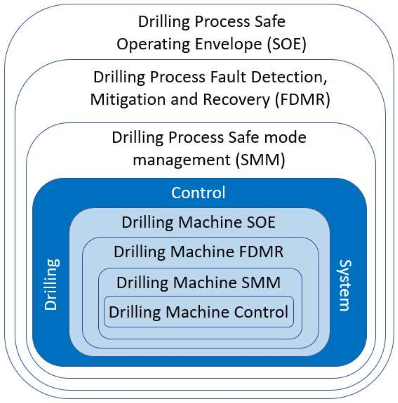
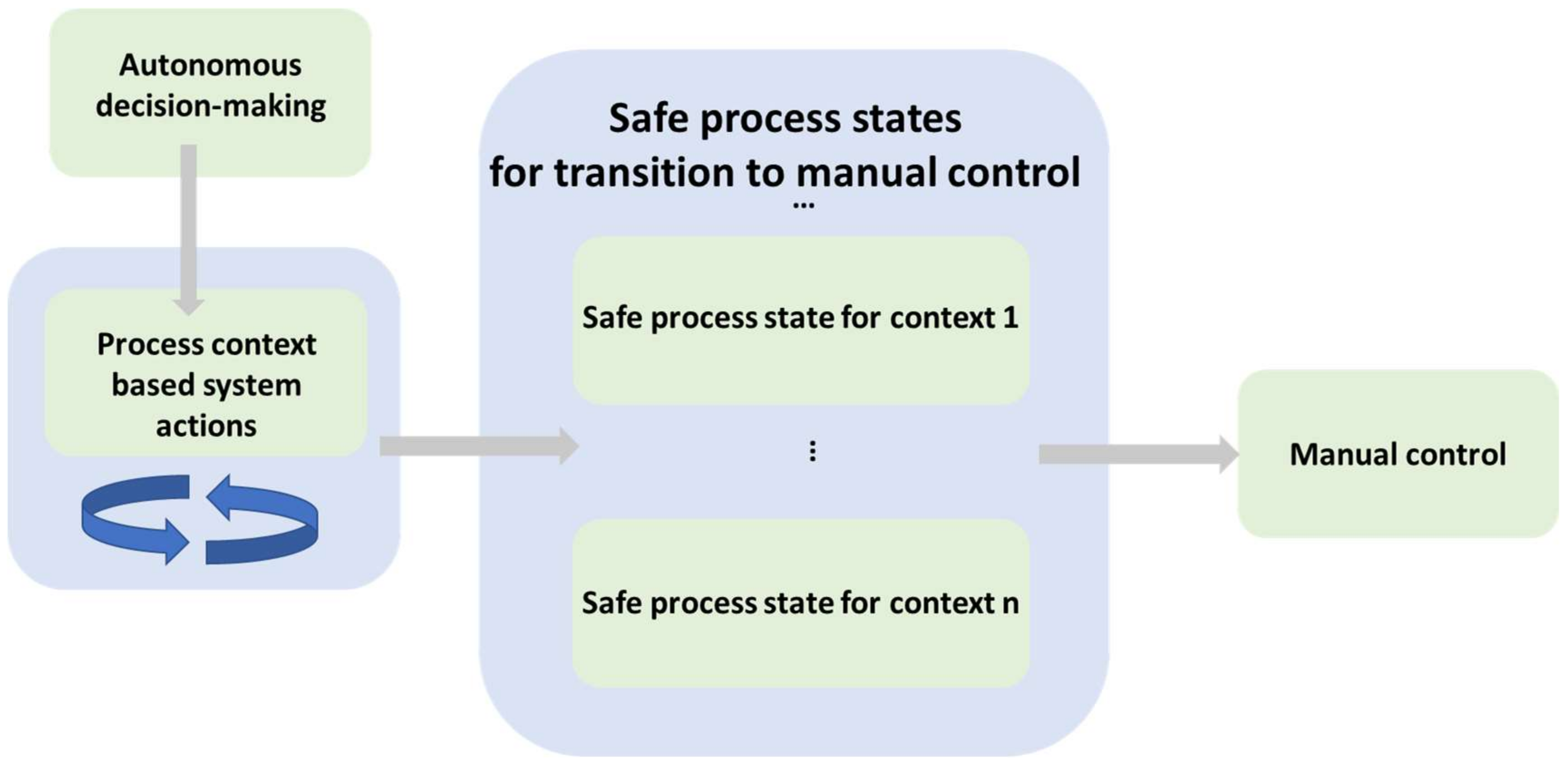
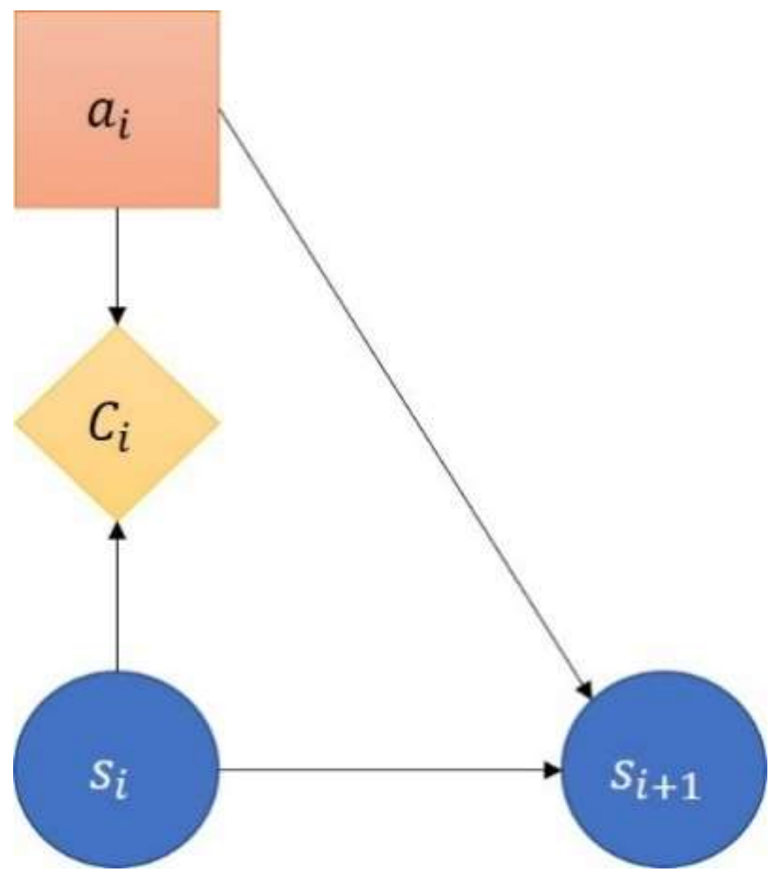
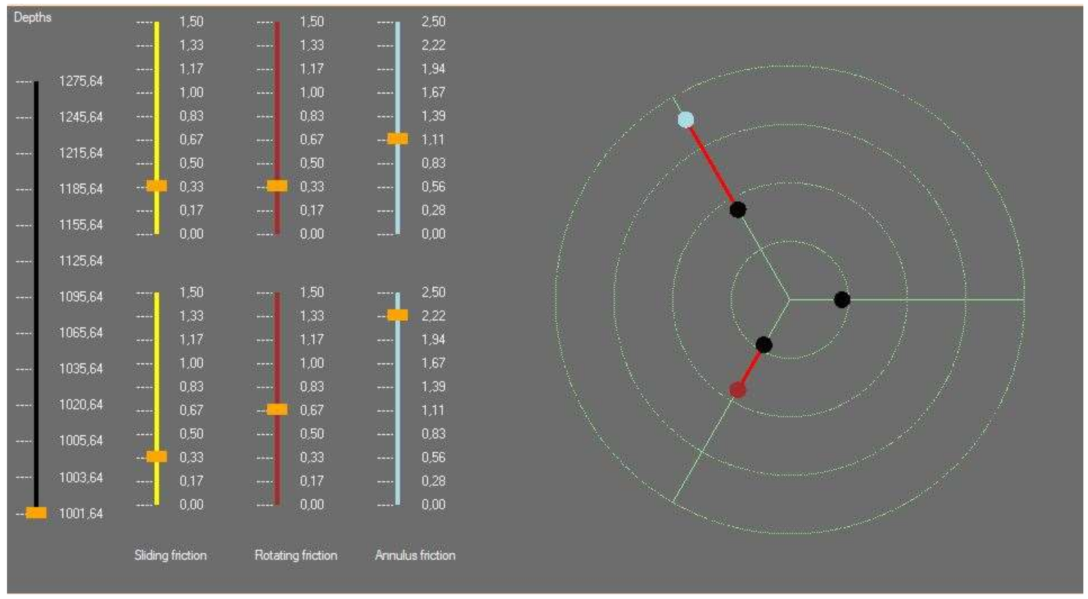
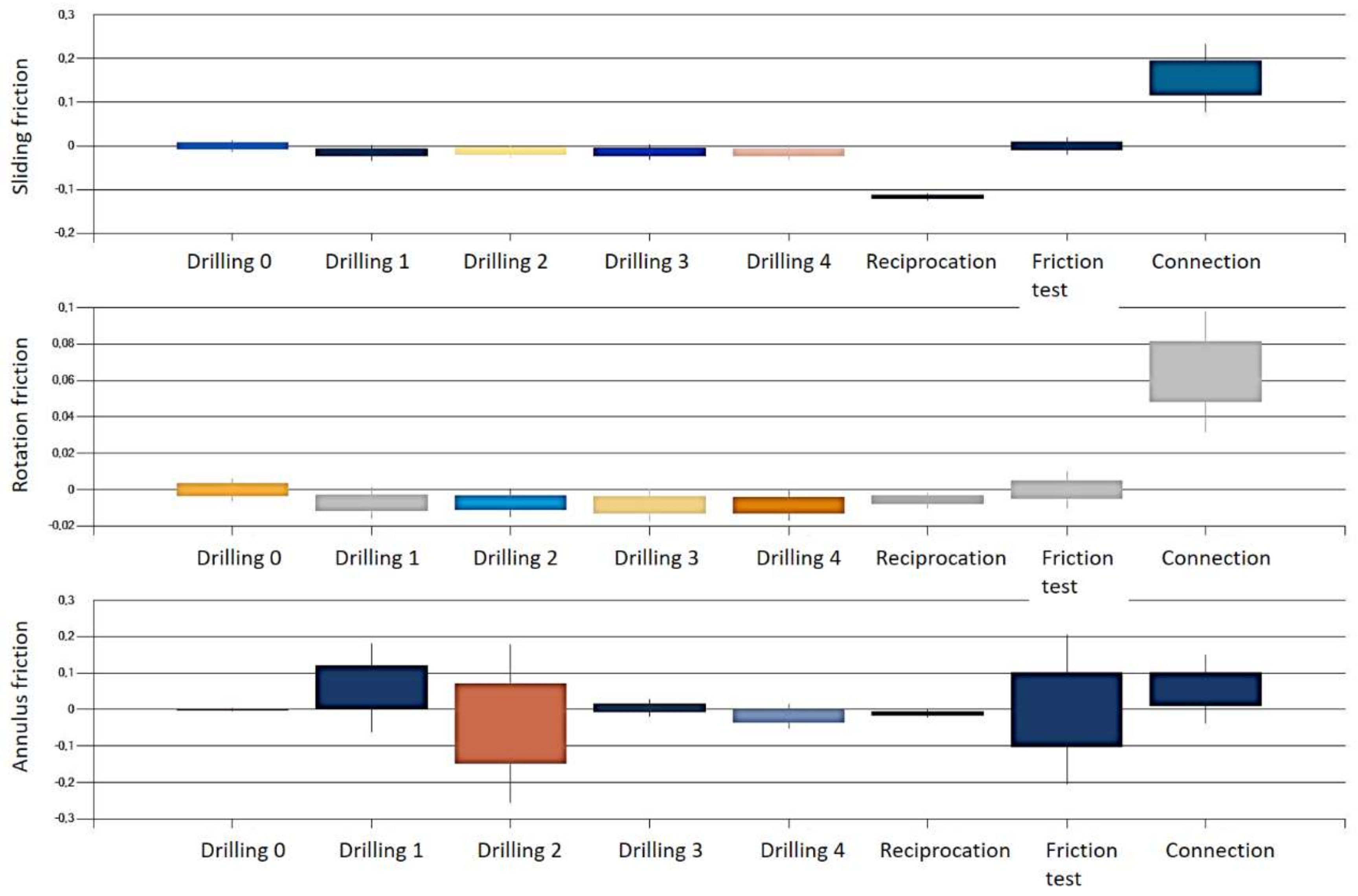
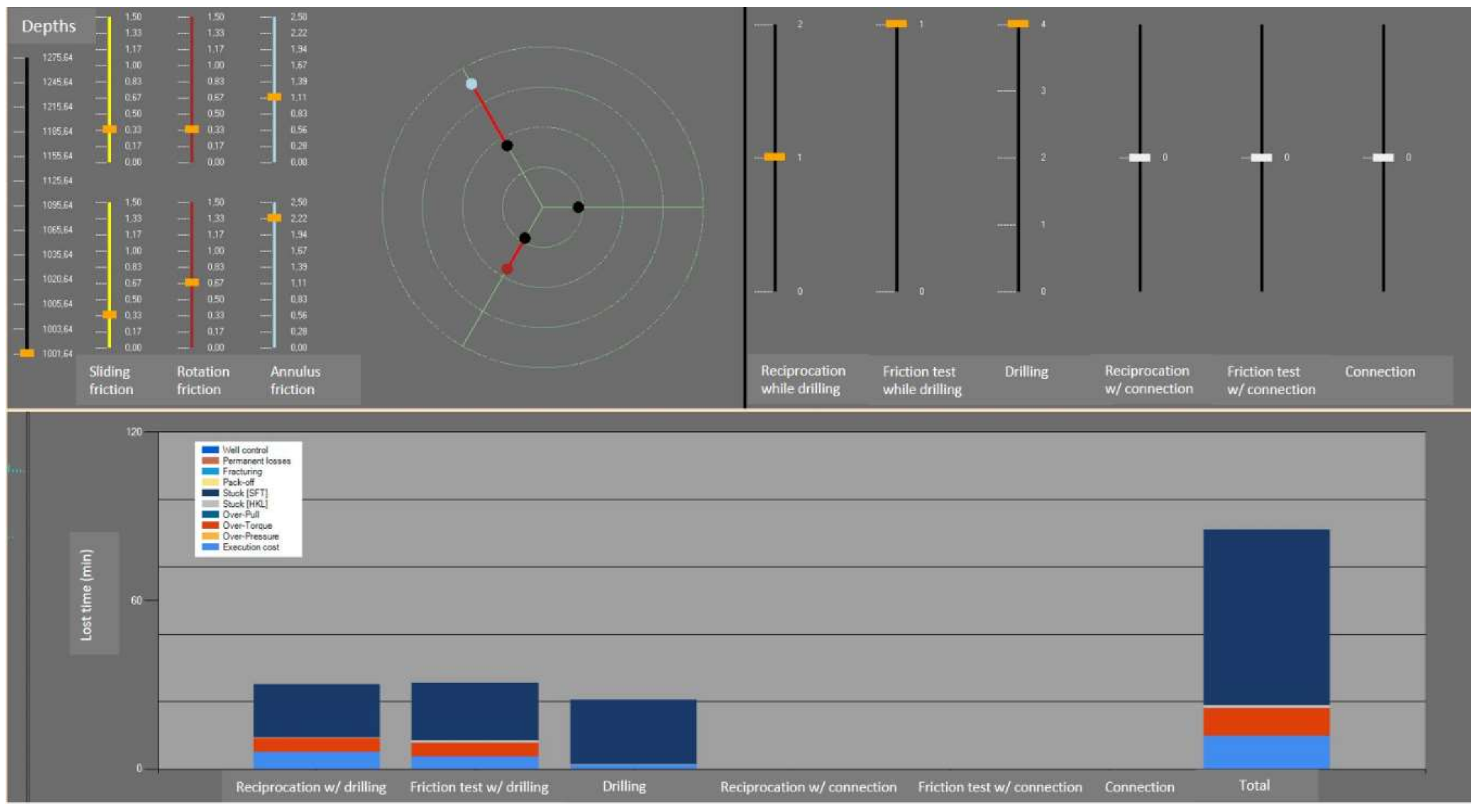
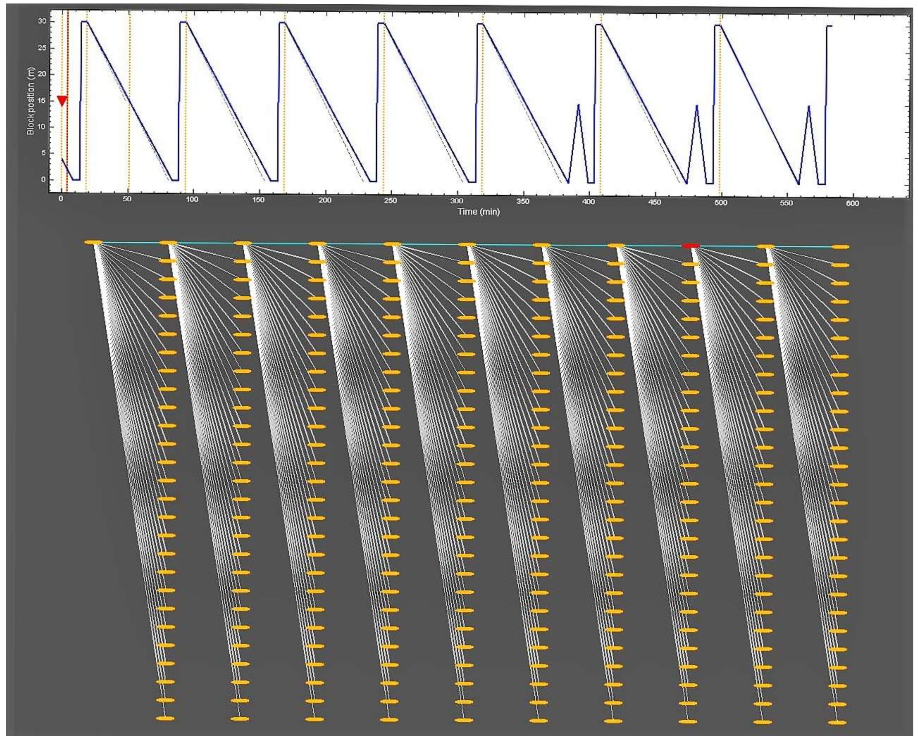
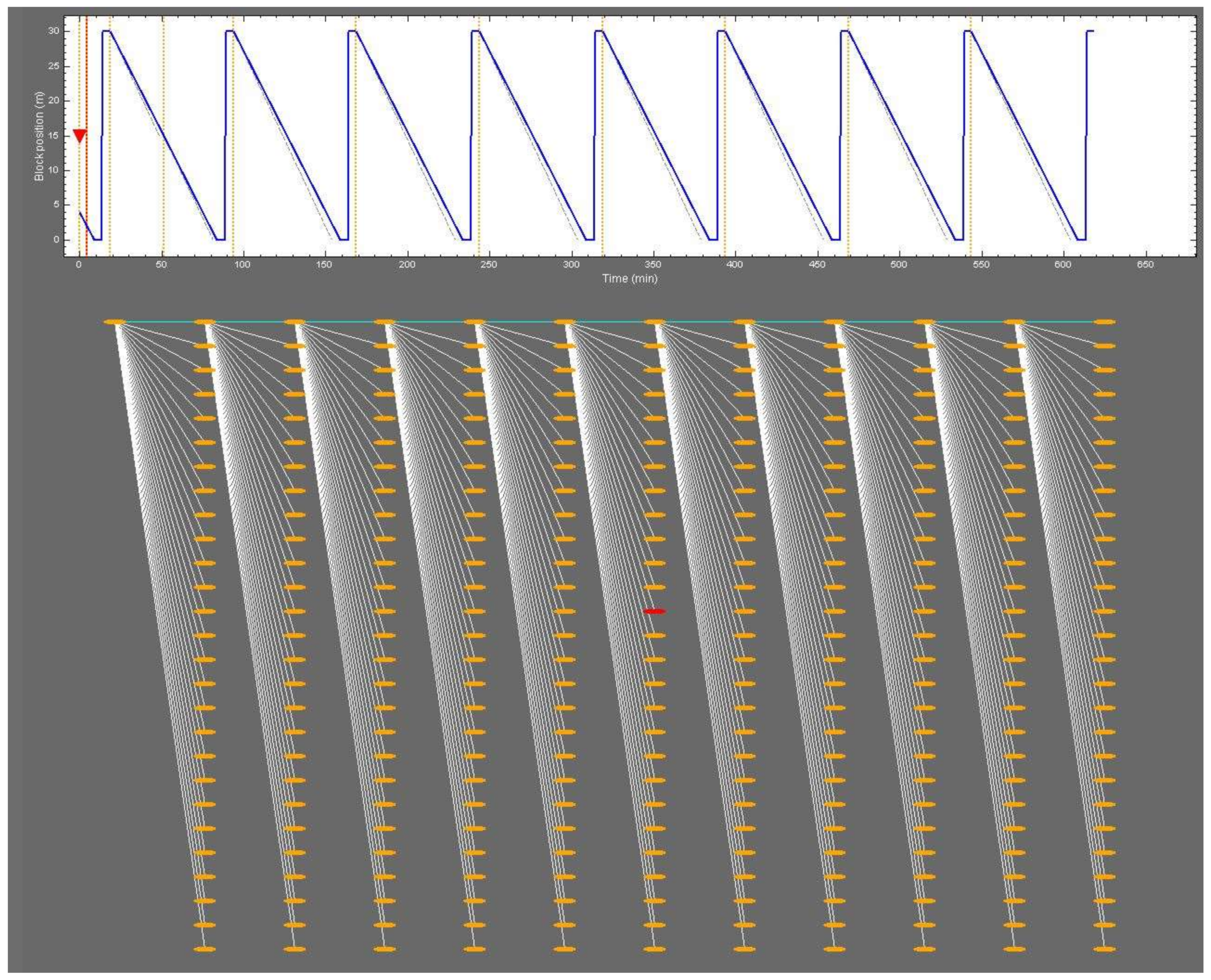
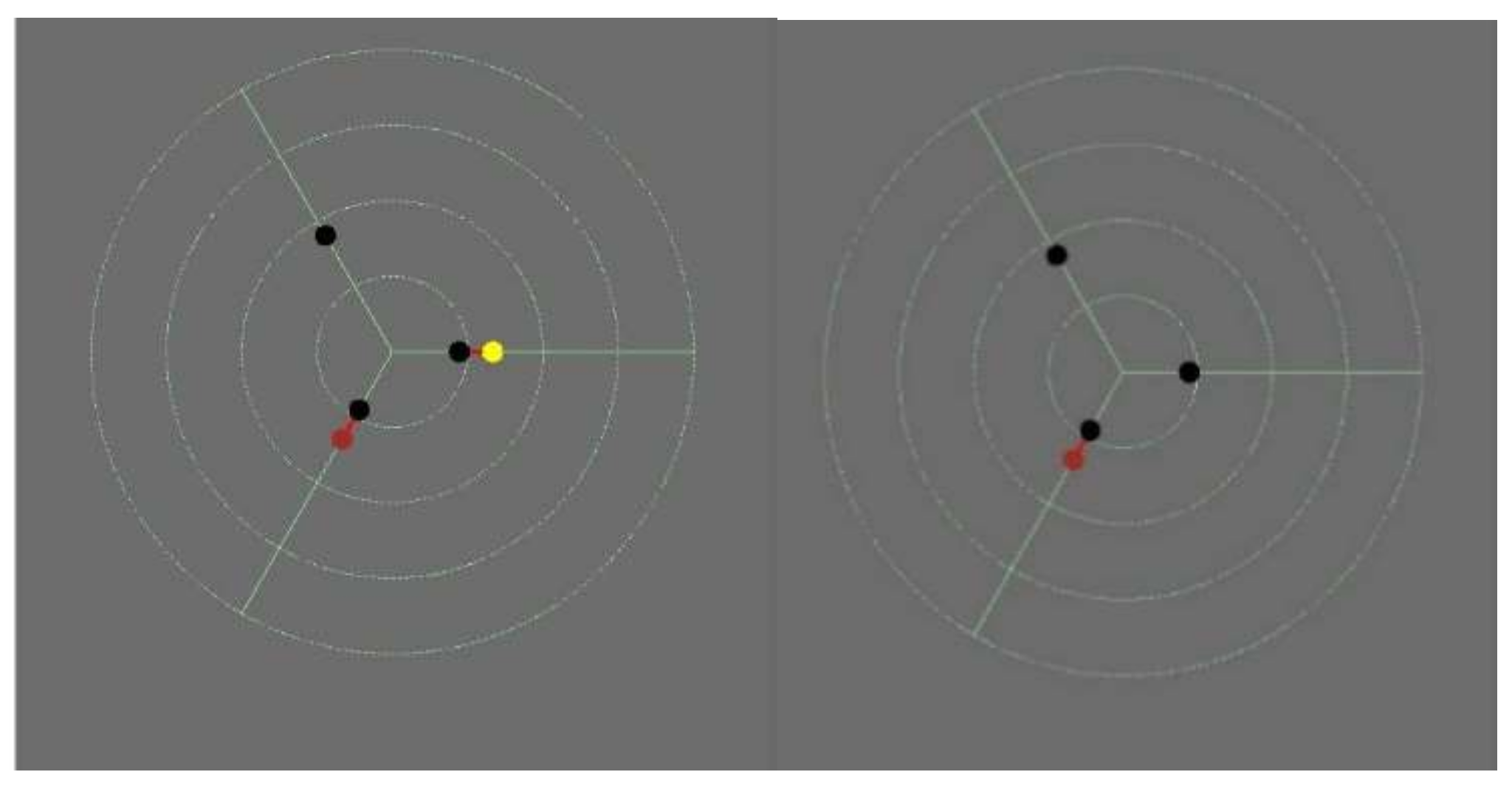
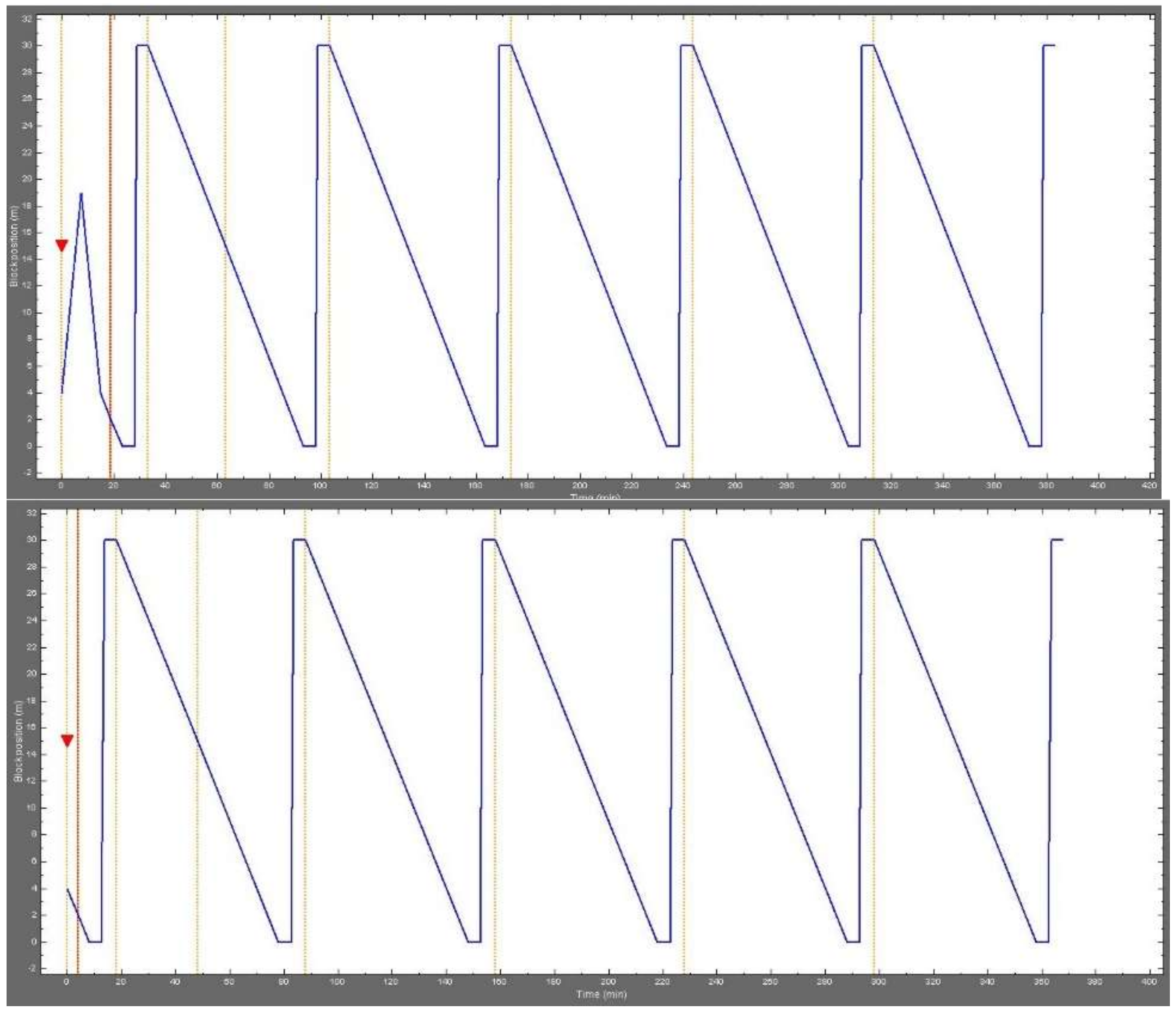
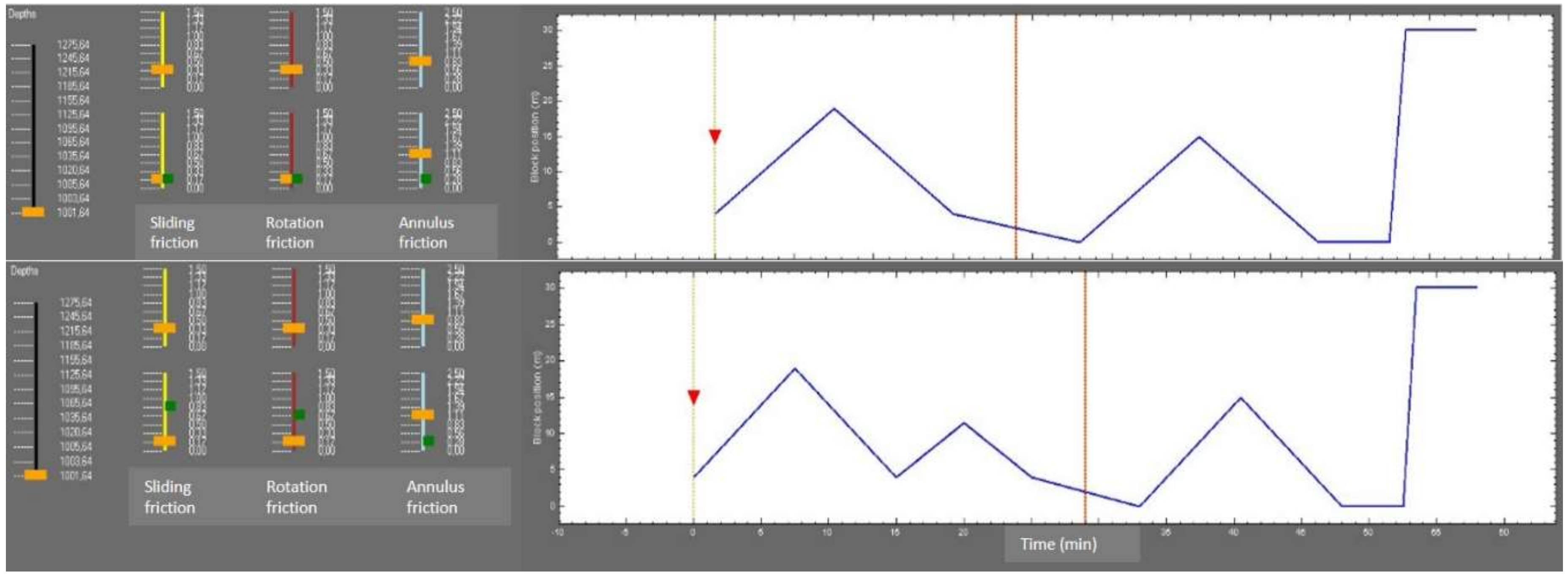