On Adaptive Moving Average Algorithms for the Application of the Conservative Power Theory in Systems with Variable Frequency

Abstract

The Conservative Power Theory (CPT) emerged in recent decades as a theoretical framework for coping with harmonically distorted and unbalanced electric networks of ac power systems with a high participation of converter interfaced loads and generation. The CPT measurements are intrinsically linked to moving averages (MA) over one period of the grid. If the CPT is to be used in a low-inertia isolated-grid scenario, which is subjected to frequency variations, adaptive moving averages (AMA) are necessary. This paper reviews an efficient way of computing MAs and turns it into an adaptive one. It shows that an easily available variable time delay block, from MATLAB, causes steady-state errors in the measurements when the grid frequency varies. A new variable time delay block is, thus, proposed. Nonetheless, natural pulsations in the instantaneous power slip through MAs when the discrete moving average window does not fit perfectly the continuously varying period of the grid. A method consisting of weighing two MAs is reviewed and a new and effective hybrid AMA is proposed. The CPT transducers with the different choices of AMAs are compared via computer simulations of a single-phase voltage source feeding either a linear or a nonlinear load.

1. Introduction

In the emerging smart-grid scenario, characterized by a growing number of converter interfaced renewable energy sources, energy storage systems, and smart load management enabled by sensors ubiquity and increased communication capabilities, the need for a theoretical framework capable of coping with distorted and unbalanced electric network was experienced. The Conservative Power Theory (CPT), first proposed in [1], emerged in recent decades as a potential framework as it aims to retain a clear physical meaning for all the different power and current terms it defines, which facilitates its use for driving compensation systems in different applications [2,3,4].

The initial formulation of the CPT [1,5] was subsequently revised [6,7] to cope with variable frequency systems. While the ongoing debate [8] on specific CPT quantities, such as the reactive energy, is beyond the scope of this paper, the revision provided by [6,7] highlights the importance of correctly characterizing electrical systems that feature a relevant penetration of power electronic converter interfaced loads and are prone to variations in their electrical frequency.

The motivation of this paper stems precisely from the application of the CPT on offshore isolated oil and gas platforms. Such platforms commonly feature a high penetration of converter interfaced loads. Furthermore, due to the presence of large motors with variable operation, these grids are prone to variations in their electrical frequency. In particular, this paper aims at contributing towards the practical use of the CPT in industrial applications by:

• highlighting how inappropriate implementations of adaptive moving average (AMA) filters can impair the calculation of the basic electrical quantities underpinning the CPT, namely the active power, reactive energy, and active, reactive, and void currents;
• proposing a new variable time delay (VTD) algorithm to be used within an AMA that corrects steady-state errors introduced by a commonly available VTD;
• proposing a new hybrid implementation of an AMA that reduces oscillations in the measurements due to discretization errors and removes small transients caused by a continuously variable frequency.

Even though the CPT applied to isolated ac grids with variable frequency is used as backdrop, the discussions and new methods proposed in this article show higher generality, as they are applicable to multiple other fields which employ AMAs.

2. CPT Measurements and Moving Averages

The CPT as presented in [7] defines a series of electrical quantities calculated via internal products. When expressed in terms of generic periodic variables $x\left(t\right)$ and $y\left(t\right)$, these internal products take the form of

$$\langle x\left(t\right),y\left(t\right)\rangle ={\displaystyle \frac{1}{T}}{\int }_{t-T}^{t}x\left(\tau \right)y\left(\tau \right)\mathrm{d}\tau ,$$

(1)

where T is the fundamental period of both variables. Equation (1) calculates a moving average (MA) of the value of x times y over the last period T.

Let a single-phase electrical circuit be fed by an ac voltage source. The instantaneous power consumed by the circuit is equal to

$$p\left(t\right)=u\left(t\right)i\left(t\right),$$

(2)

where $u\left(t\right)$ and $i\left(t\right)$ are the instantaneous voltage and current supplied to the circuit. If u is sinusoidal and the electrical system is linear, the waveform of p is also sinusoidal but with twice the frequency of u. The dc-level of the sinusoidal p depends on the phase shift between u and i. From the perspective of the thermal design of electrical components, it makes little sense to evaluate heat dissipation on the time scale of the instantaneous power, i.e., twice the grid frequency. A more useful measurement is, instead, the average of p over the last period T. This measurement is called active power and is applicable to sinusoidal and nonsinusoidal cases, as well as to linear and nonlinear circuits.

The CPT defines the active power $\overline{p}\left(t\right)$ as

$$\overline{p}\left(t\right)=\langle u\left(t\right),i\left(t\right)\rangle .$$

(3)

Notice the use of the internal product from Equation (1). The active power $\overline{p}\left(t\right)$ is, therefore, a MA of the instantaneous power with a moving average window (MAW) equal to T. To calculate $\overline{p}\left(t\right)$, one needs to know the electrical system’s frequency.

The CPT defines also a quantity for a periodic distorted condition named reactive energy, $\overline{w}$ in Equation (4). This quantity does not use directly the voltage u. It uses, instead, an unbiased integral of the voltage calculated with Equation (5), which is equal to the integral of the voltage from instant zero to t, see Equation (6), minus the MA of this same integral between times $t-T$ and t.

$$\overline{w}\left(t\right)=\langle \stackrel{⌢}{u}\left(t\right),i\left(t\right)\rangle$$

(4)

$$\stackrel{⌢}{u}\left(t\right)=u_{\int }\left(t\right)-{\displaystyle \frac{1}{T}}{\int }_{t-T}^t{u}_{\int }\left(\tau \right)\mathrm{d}\tau$$

(5)

$$u_{\int }\left(t\right)={\int }_0^{t}u\left(t\right)\mathrm{d}t$$

(6)

The more commonly known reactive power is defined by the CPT as

$$\overline{q}\left(t\right)={\displaystyle \frac{\sqrt{\langle u\left(t\right),u\left(t\right)\rangle }}{\sqrt{\langle \stackrel{⌢}{u}\left(t\right),\stackrel{⌢}{u}\left(t\right)\rangle }}}\overline{w}\left(t\right).$$

(7)

For a sinusoidal $u\left(t\right)$, Equation (7) can be simplified to

$$\overline{q}\left(t\right)=\omega \overline{w}\left(t\right),$$

(8)

where $\omega =2\pi /T$. As the computer simulation test setup in Section 8 features only an ideal sinusoidal voltage source, the simplified Equation (8) is going to be used throughout the paper for calculating the reactive power.

When it comes to power quality and compensation, the CPT defines an active ($i_a$), a reactive ($i_r)$, and a void current ($i_v$), which are shown below:

$$i_a\left(t\right)={\displaystyle \frac{\overline{p}\left(t\right)}{\langle u\left(t\right),u\left(t\right)\rangle }}u\left(t\right)={\displaystyle \frac{\overline{p}\left(t\right)}{{\parallel u\left(t\right)\parallel }^2}}u\left(t\right),$$

(9)

$$i_r\left(t\right)={\displaystyle \frac{\overline{w}\left(t\right)}{\langle \stackrel{⌢}{u}\left(t\right),\stackrel{⌢}{u}\left(t\right)\rangle }}\stackrel{⌢}{u}\left(t\right)={\displaystyle \frac{\overline{w}\left(t\right)}{\parallel \stackrel{⌢}{u}{\left(t\right)\parallel }^2}}\stackrel{⌢}{u}\left(t\right),$$

(10)

$$i_v\left(t\right)=i\left(t\right)-i_a\left(t\right)-i_r\left(t\right).$$

(11)

Notice that the internal product of a variable by itself is also called the norm squared (${\parallel .\parallel }^2$) of this variable.

3. Moving Averages in the Discrete Time Domain

All CPT measurements shown previously are defined in the continuous time domain. However, a real implementation of a CPT transducer would most certainly run in an electronic microprocessor with a fixed sampling frequency $f_s$ and fixed sampling time $T_s=1/f_s$. In this paper, the time in the discrete domain is represented by an ever-increasing index k. Moreover, the terms time, sample, or cycle k referring to an instant $k{T}_s$ are interchangeably employed. Furthermore, the operator that fetches the value of a variable at the $r^{\mathrm{th}}$ previous cycle is denoted by $z^{-r}$.

The MAs in the CPT measurements need to be calculated in the discrete time domain. One inefficient way of doing this is by a series of sums:

$$\overline{x}\left(k\right)={\displaystyle \frac{1}{N}}\sum _{r=0}^{N-1}x\left(k\right)z^{-r},$$

(12)

where $x\left(k\right)$ represent a generic variable and $\overline{x}\left(k\right)$ its MA and N is the number of samples acquired in one period T of the grid. If one expands Equation (12), multiplies it by $\frac{1-z^{-1}}{1-z^{-1}}$, and rearranges the numerator, the result is

$$\overline{x}\left(k\right)={\displaystyle \frac{x\left(k\right)}{N}}{\displaystyle \frac{\left(z^0+\cdots +z^{-N+1}\right)-\left(z^{-1}+\cdots +z^{-N}\right)}{1-z^{-1}}}.$$

(13)

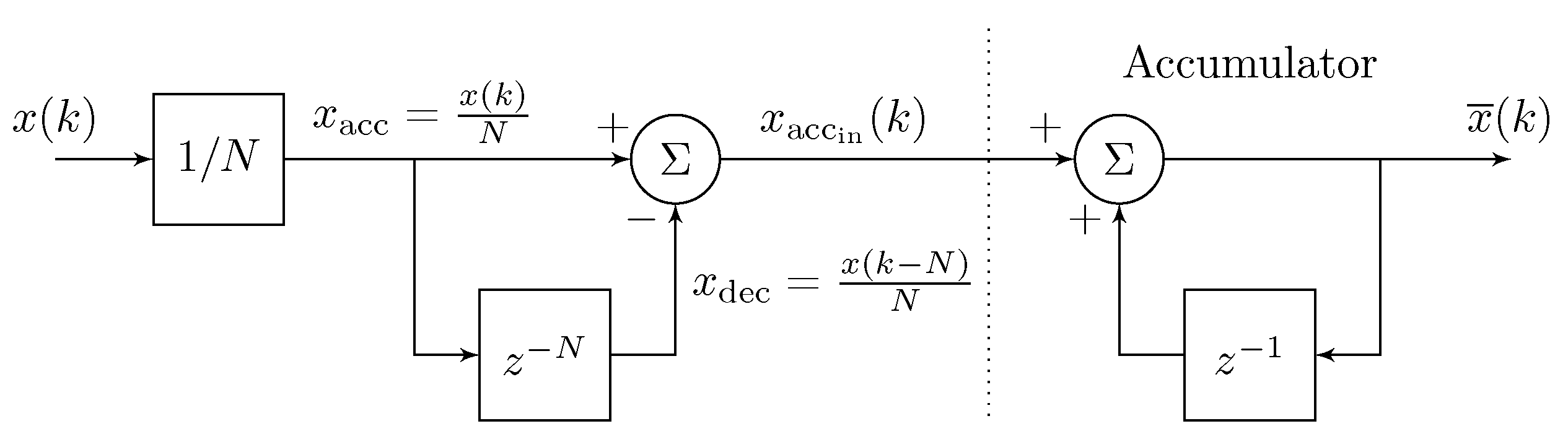
Most of the terms in Equation (13) can be canceled, yielding Equation (14) [9] (p. 394). Figure 1 shows one possible block diagram representation of Equation (14) adapted from [10]. It is important to remark that even though computationally efficient, Equation (14) still demands the last N samples of x to be stored in memory.

$$\overline{x}\left(k\right)={\displaystyle \frac{x\left(k\right)}{N}}{\displaystyle \frac{1-z^{-N}}{1-z^{-1}}}$$

(14)

4. Adaptive Moving Averages

The diagram in Figure 1 is divided by a dotted line. To the right of this line there is an accumulator. The summation block to the left of the dotted line sends $x_{acc}=x\left(k\right)/N$ for accumulation, notice the positive sign, whereas $x_{dec}=x(k-N)/N$ is sent for decumulation. All values $x\left(k\right)/N$ are accumulated at the instant k and must be decumulated at a later instant $k+N$. This is a key principle into designing an AMA block.

To build an AMA from the diagram in Figure 1, one needs to turn the constant MAW N into a variable one

$$n\left(k\right)=\frac{f_s}{f\left(k\right)},$$

(15)

where $f_s$ is the sampling frequency with which the CPT is processed and $f\left(k\right)$ is the measured fundamental frequency of the electrical grid. However, the discrete delay N in $z^{-N}$ must be an integer. A natural choice is to round $n\left(k\right)$ to the closest integer

$$n_r\left(k\right)=\mathrm{round}\left(n\left(k\right)\right).$$

(16)

To maintain consistency, $n_r$ replaces N in both gain $1/N$ and discrete delay $z^{-N}$ in Figure 1.

A key element for calculating the AMA is the VTD block ($z^{-n_r}$) which is typically implemented with a circular buffer. See [9] for more information on hardware realizations and circular buffers. The length of the buffer, named $N_b$, needs to be large enough to store all samples of $x/n_r$ during the longest periods of the grid, i.e., when the frequency is at its minimum. Two pointers control the insertion of data into the buffer and the retrieval of information from the buffer:

• j points to where the current $x/n_r$ is to be stored; it is purposefully named j for avoiding the confusion with the current i;
• r points to the slot from which the old value of $x/n_r$ is to be retrieved.

In this paper, two strategies for handling the pointers will be analyzed. The first one uses a readily available VTD from [11] which introduces steady-state errors into the CPT measurements when the grid frequency changes. The second one, proposed by this paper, does not introduce steady-state errors.

4.1. Lossy Variable Time Delay Block

The insertion pointer of the VTD from [11] marches continuously forward through the circular buffer one step per cycle time $T_s$. The value of j is calculated by the remainder of the division (mod) of the time k by $N_b$, see Equation (17). The old content of the slot pointed by j is replaced by the new value. The retrieval pointer r lags one MAW number of slots behind j, see Equation (18). The old value is retrieved from the slot pointed by r. The buffer slot is left intact after retrieval.

$$j\left(k\right)=kmod{N}_b$$

(17)

$$r\left(k\right)=(k-n_r\left(k\right))mod{N}_b$$

(18)

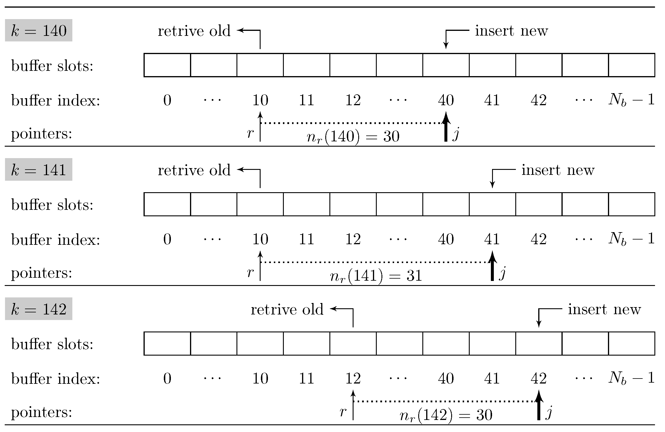
The retrieval pointer is forced to skip slots, stay put, or jump backwards whenever the MAW changes as r is pulled $n_r$ slots behind j. If the grid frequency increases, $n_r$ decreases, and old values of $x/n_r$ are skipped. The opposite happens when the grid frequency decreases, $n_r$ increases, the retrieval pointer jumps backwards, and old values of $x/n_r$ are retrieved twice.

Figure 2 shows one instance of a skipped decumulation and one of a double decumulation. From time $k=140$ to $k=141$, the grid frequency decreases causing the MAW to increase. The retrieval pointer remains at slot 10 causing a double decumulation. From time $k=141$ to $k=142$, the dual problem happens. The grid frequency increases, $n_r$ decreases, and slot 11 is skipped.

It is important to recall Figure 1. When a value $x/n_r$ enters the accumulator of the MA, it must be decumulated $n_r$ cycles later. If this value is not decumulated or is sent twice for decumulation, the accumulator will bear a steady-state error. Due to the missed and double decumulations caused by the VTD from [11], it is called in this paper the lossy variable time delay (LVTD).

4.2. Conservative Variable Time Delay Block

A new VTD is proposed in this section. The retrieval pointer r of this new block is the one continuously moving forward whereas the insertion pointer j is pushed $n_r$ slots ahead of r. It is the insertion pointer, not the retrieval, that is forced to jump or stay put whenever the MAW is updated. The other necessary changes are: (1) sum to the content of the slot when inserting and (2) set the slot to zero after retrieval. The new insertion and retrieval pointers behave according to Equations (19) and (20).

$$j\left(k\right)=(k+n_r\left(k\right))mod{N}_b$$

(19)

$$r\left(k\right)=kmod{N}_b$$

(20)

Every value entering this new VTD is ensured to be decumulated only once even when the grid frequency decreases. No values are lost either when the frequency increases. For this reason, the new block is named conservative variable time delay (CVTD).

5. CPT Measurements in the Discrete Time Domain

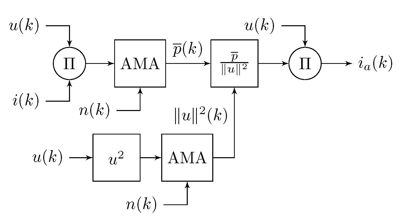
Two VTDs for performing AMAs were presented in the previous sections. It is now convenient to represent the calculation of the CPT electrical quantities in the discrete time domain. Figure 3 shows a block diagram of the active power and active current measurements given by Equations (3) and (9). One AMA is used for $\overline{p}$ and another one is used for ${\parallel u\parallel }^2$. The active current $i_a$ depends on both AMAs.

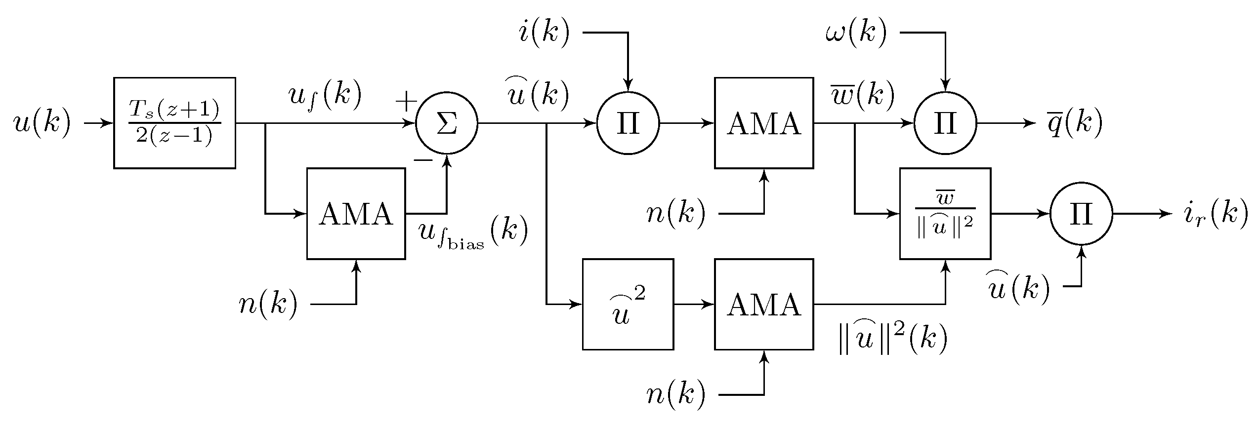
Figure 4 shows the block diagram representation of the measurement of the reactive energy, reactive power, and the reactive current given by Equations (4), (8) and (10). The reactive energy depends on $\stackrel{⌢}{u}$ from Equation (5) which in turn depends on $u_{\int }$ from Equation (6). The trapezoidal approximation is chosen for calculating $u_{\int }$:

$$u_{\int }\left(k\right)=\frac{T_s(z+1)}{2(z-1)}u\left(k\right).$$

(21)

This approximation provides a better accuracy than the forward and backward rectangular methods [12]. Nevertheless, the analysis of different choices of discrete integration and their effects on $u_{\int }$, $\overline{w}$, $\overline{q}$, $i_r$, and $i_v$ are considered beyond the scope of this paper.

Cascaded AMAs are needed for calculating $\overline{w}$, $\overline{q}$, $i_r$, and $i_v$. The consequences of this can be seen in Section 9.1.1. It is important to recall that the reactive power shown in Figure 4 is obtained from the simplified Equation (8). In other words, it is valid for sinusoidal voltages. The reactive energy and current, on the other hand, are valid for distorted voltages as well. Furthermore, the angular frequency is calculated from the measured grid frequency, i.e., $\omega \left(k\right)=2\pi f\left(k\right)$.

6. Weighted Adaptive Moving Average

The processing and memory requirements for a CPT transducer built with either LVTDs or CVTDs are similar. Furthermore, as it is shown in Section 9, the poor performance of the transducer with LVTDs discourages their use. However, both CPT transducers with LVTDs and CVTDs let through a noticeable parcel of the pulsations in $ui$ and $\stackrel{⌢}{u}i$ when the grid frequency varies continuously.

The AMAs behave as filters removing oscillations with a frequency equal to or a multiple of $1/\left(n_r{T}_s\right)$ [13] (p. 341). When the period of the grid T is not equal to $n_r{T}_s$, the AMAs do not block completely the fundamental frequency $1/T$ and its harmonics [14]. To mitigate this problem, a weighting of MAs proposed by [15] can be used. This method calculates two MAs and is named weighted adaptive moving average (WAMA) in this paper.

The output of the WAMA, ${\overline{x}}_w\left(k\right)$ in Equation (22), is composed by the weighted sum of two AMAs. The first one, ${\overline{x}}_c\left(k\right)$, uses a window equal to the value of $n\left(k\right)$ rounded up to the closest integer as shown by Equation (23). The second one, ${\overline{x}}_f\left(k\right)$, rounds the window down to the closest integer as shown by Equation (24). The terms ceiling is used for rounding up and floor for rounding down.

$${\overline{x}}_w\left(k\right)=\left(n\left(k\right)-n_f\left(k\right)\right){\overline{x}}_c\left(k\right)+\left(1-n\left(k\right)+n_f\left(k\right)\right){\overline{x}}_f\left(k\right)$$

(22)

$$n_c\left(k\right)=\mathrm{ceiling}\left({\displaystyle \frac{f_s}{f\left(k\right)}}\right)$$

(23)

$$n_f\left(k\right)=\mathrm{floor}\left({\displaystyle \frac{f_s}{f\left(k\right)}}\right)$$

(24)

It is important to remark that a CPT measurement transducer for a single-phase circuit uses five AMAs, see Figure 3 and Figure 4, which may be a burden for real applications. However, in addition to other functions, modern microprocessors are capable of handling the CPT computational demands for single-phase and for three-phase four-legged converters as seen in the experimental results obtained by [16,17]. A WAMA uses twice as much memory than a single AMA. Nevertheless, this is not considered a critical barrier for implementing the WAMA in a CPT transducer.

7. Hybrid Adaptive Moving Average

As it will be shown in Section 9, the CPT transducer built with WAMAs reduces the oscillations due to unmatched $n_r{T}_s$ and T. However, it still features unwanted transients whenever the MAW is updated. It is interesting to notice that when the grid frequency varies in a continuous way, $n_c$ and $n_f$ are not updated at the same time as $n_r$. Thus, this article proposes a hybrid adaptive moving average (HAMA) that exploits this fact. The following strategy is employed:

• three internal AMAs: ${\overline{x}}_r$ with rounded window from Equation (16), ${\overline{x}}_c$ with ceiling window from Equation (23), and ${\overline{x}}_f$ with floor window from Equation (24);
• the block usually outputs: ${\overline{x}}_w$ from Equation (22),
• but at the cycle in which $n_c$ changes and for $n_c\left(k\right)$ cycles after that, the hybrid block outputs: ${\overline{x}}_r$.

It is important to remark that the HAMA demands 50% more memory than the WAMA.

8. Materials and Methods

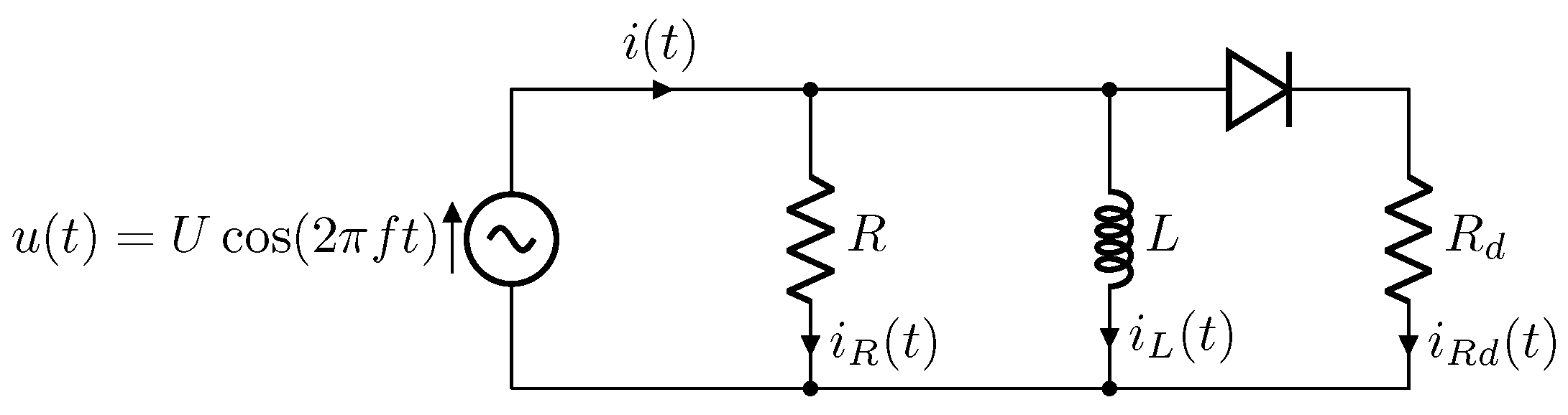
The effects of the LVTD and CVTD in the measurements of a CPT transducer are analyzed in this paper with the help of computer simulations. The comparisons between a single AMA with rounded MAW, a WAMA, and a HAMA are also performed with simulations. To do that, a single-phase ideal sinusoidal voltage source feeding a relatively simple load is chosen. The load is composed of ideal components: one resistor R, one inductance L, and one diode in series with a resistor $R_d$. Figure 5 shows the test model.

The instantaneous value of the source voltage in Figure 5 is calculated with the cosine of $2\pi ft$ with the frequency in $\mathrm{Hz}$ and the time in $\mathrm{s}$. This is done on purpose so the simulation can start with initial conditions set to zero and, still, result in zero steady-state dc-level at $i_L$. It is important to mention that changes in the sinusoidal profile of u can induce a dc-level in $i_L$. Furthermore, as u is sinusoidal, a dc-level in $i_L$ is reflected as a dc-level in the void current after the CPT decomposes i.

The analysis is performed with two load scenarios. The first one is resistive and inductive (RL), i.e., the resistance $R_d$ in Figure 5 is disconnected. The second scenario features a diode bridge (DB), the resistance R and the inductance L are disconnected. Those two simple scenarios were chosen so the effects of the different choices of AMAs in the reactive and void currents can be highlighted. The tests are composed of simple disturbances applied to the frequency f in Figure 5 while the system is in steady state. Errors introduced in the void current are highlighted in the RL-scenario as $i_v$ is expected to be zero before the disturbances. Conversely, errors in $i_r$ are highlighted in the DB-scenario. The computer simulation data is shown in

Table 1. Computer simulation data for the rl-load and db-load scenarios.

	rl-Load Scenario	db-Load Scenario
Source voltage amplitude U	$\sqrt{2}\mathrm{V}$	$\sqrt{2}\mathrm{V}$
Source frequency f (pre-disturbance)	$50\mathrm{Hz}$	$50\mathrm{Hz}$
Load resistance R	$2\Omega$	disconnected
Load inductance L	$6.3662\mathrm{m}\mathrm{H}$	disconnected
db-load resistance $R_d$	disconnected	$1\Omega$
Transducer sampling frequency $f_s$	$20\mathrm{k}\mathrm{Hz}$	$20\mathrm{k}\mathrm{Hz}$

and the expected steady-state measurements are found in

Table 2. Expected pre-disturbance steady-state measurements for the rl-load and db-load scenarios.

	RL-Load Scenario	DB-Load Scenario
Active power $\overline{p}$	$0.5\mathrm{W}$	$0.5\mathrm{W}$
Reactive power $\overline{q}$	$0.5\mathrm{Var}$	$0\mathrm{Var}$
Active current $i_a$ (min to max)	$-0.5\sqrt{2}$ to $0.5\sqrt{2}\mathrm{A}$	$-0.5\sqrt{2}$ to $0.5\sqrt{2}\mathrm{A}$
Reactive current $i_r$ (min to max)	$-0.5\sqrt{2}$ to $0.5\sqrt{2}\mathrm{A}$	$0\mathrm{A}$
Void current $i_v$ (min to max)	$0\mathrm{A}$	0 to $0.5\sqrt{2}\mathrm{A}$

.

The CPT algorithm is simulated in the discrete time domain with a fixed cycle time $T_s$ and sampling frequency $f_s=1/T_s$. At the beginning of each processing cycle, the source’s voltage, current, and frequency are sampled simultaneously. There is no delay nor noise in the measurements. The sampled values are hold constant throughout one complete calculation of the transducer’s algorithm, as usual in microprocessor implementations. Intentional variable sampling times, unintentional variations of the main software cycle time, or non-simultaneous sampling of the voltage and current are beyond the scope of this paper.

9. Results

This section is subdivided into two. Firstly, a subsection comparing the effects of single AMAs with rounded MAWs using either LVTDs or CVTDs. Secondly, a comparison between single AMAs with rounded MAWs versus WAMAs versus HAMAs.

9.1. LVTD versus CVTD

Two CPT transducers using either LVTDs or CVTDs with rounded MAWs are compared in this subsection. The results of three tests are shown and commented: first, negative steps at the grid frequency for the RL-scenario; second, positive steps for the DB-scenario; and third, a continuously varying frequency for both load scenarios.

9.1.1. Negative Steps for the RL-Load

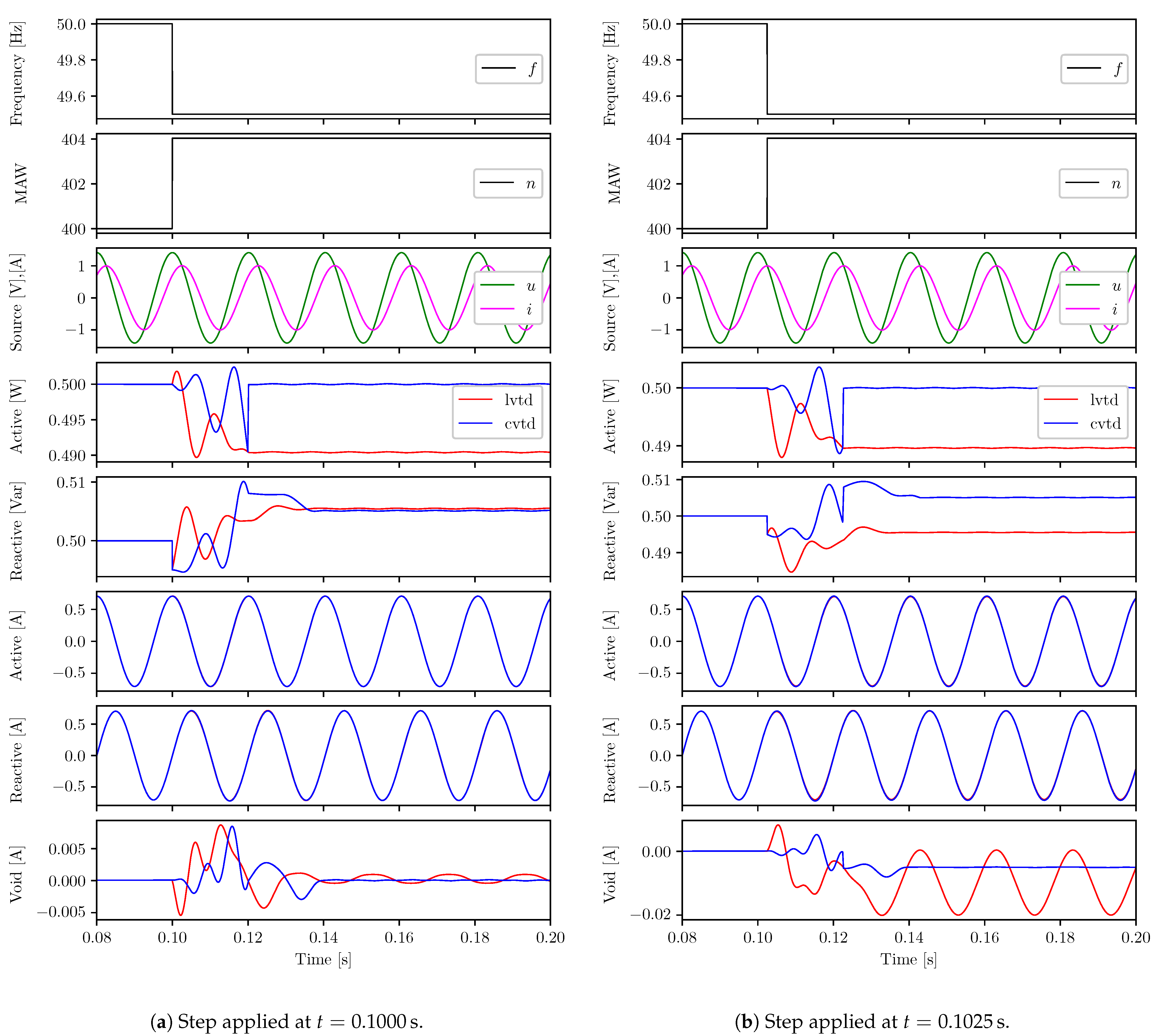
The sampling frequency of the transducers is $20\mathrm{k}\mathrm{Hz}$, see Table 1, which results in 400 samples per period of the source voltage. The negative step is precisely calculated to increase the MAWs from 400 to 404. Figure 6 shows the results of two negative steps applied at slightly different times. The measurements with LVTDs are in red. The measurements with CVTDs are in blue.

Frequency, MAW, and source voltage and current: in Figure 6a, the step is applied at the peak of the source voltage, $t=0.1\mathrm{s}$. In Figure 6b, the step in the frequency is applied $2.5\mathrm{m}\mathrm{s}$ after the peak of the voltage. The MAWs are updated immediately to 404 when the frequency changes.

Active power: should be constant at $0.5\mathrm{W}$ irrespective of the frequency step. The retrieval pointers in the LVTDs jump back and go twice over four slots after the MAW increases from 400 to 404. The values in these slots are decumulated twice introducing a steady-state error in the active power. The error is on the range of 1% of a full scale of $1\mathrm{W}$ in Figure 6a,b. The CVTDs do not cause double decumulations. After the transient period of $20\mathrm{m}\mathrm{s}$, the CVTDs auto correct the active power measurement back to $0.5\mathrm{W}$. Both measurements with LVTDs and CVTDs feature a transient. After the MAW changes from 400 to 404, the MAs have to decumulate old values of $x/400$ while accumulating new values of $x/404$ for one period of the grid, this is the cause of the transient.

Reactive power: should increase after the frequency decreases. The measurement with CVTDs settles at the expected value after a transient of $40\mathrm{m}\mathrm{s}$. Notice that the transient lasts for two periods of the grid as the reactive power measurement depends on two cascaded AMAs. The steady-state errors introduced by the LVTDs depend on which slots of the circular buffers are decumulated twice. This effect is noticeable when comparing the reactive power in red in Figure 6a,b. For the step at the crest of the source voltage, the error is barely noticeable, whereas it is approximately 1% of a full scale of $1\mathrm{Var}$ for the step at $t=0.1025\mathrm{s}$.

Active current: is expected to be sinusoidal and in phase with the source voltage. The errors introduced in the calculation of the active power by the LVTDs affect the active current. However, neither the transients nor the steady-state measurement errors are noticeable at the scale the curves are shown.

Reactive current: is expected to be sinusoidal lagging the source voltage by 90 degrees. As with the case of the active current, neither the effects of the transients nor the steady-state errors in the reactive power are noticeable in the reactive current curves.

Void current: also experiences a two-period transient due to the cascaded AMAs in the reactive energy. It is expected to be zero for the step at the crest of the source voltage. Figure 6a shows that the CPT transducer with CVTDs reacts as expected. However, the transducer with the LVTDs features a small oscillation around zero. The step at instant $t=0.1025\mathrm{s}$ introduces a dc-level in $i_L$ (refer to Figure 5). This is reflected as a dc-level in the void current. The measurement with CVTDs behave as expected in Figure 6b. However, the measurement with LVTDs oscillates noticeably with $50\mathrm{Hz}$.

9.1.2. Positive Steps for the DB-Load

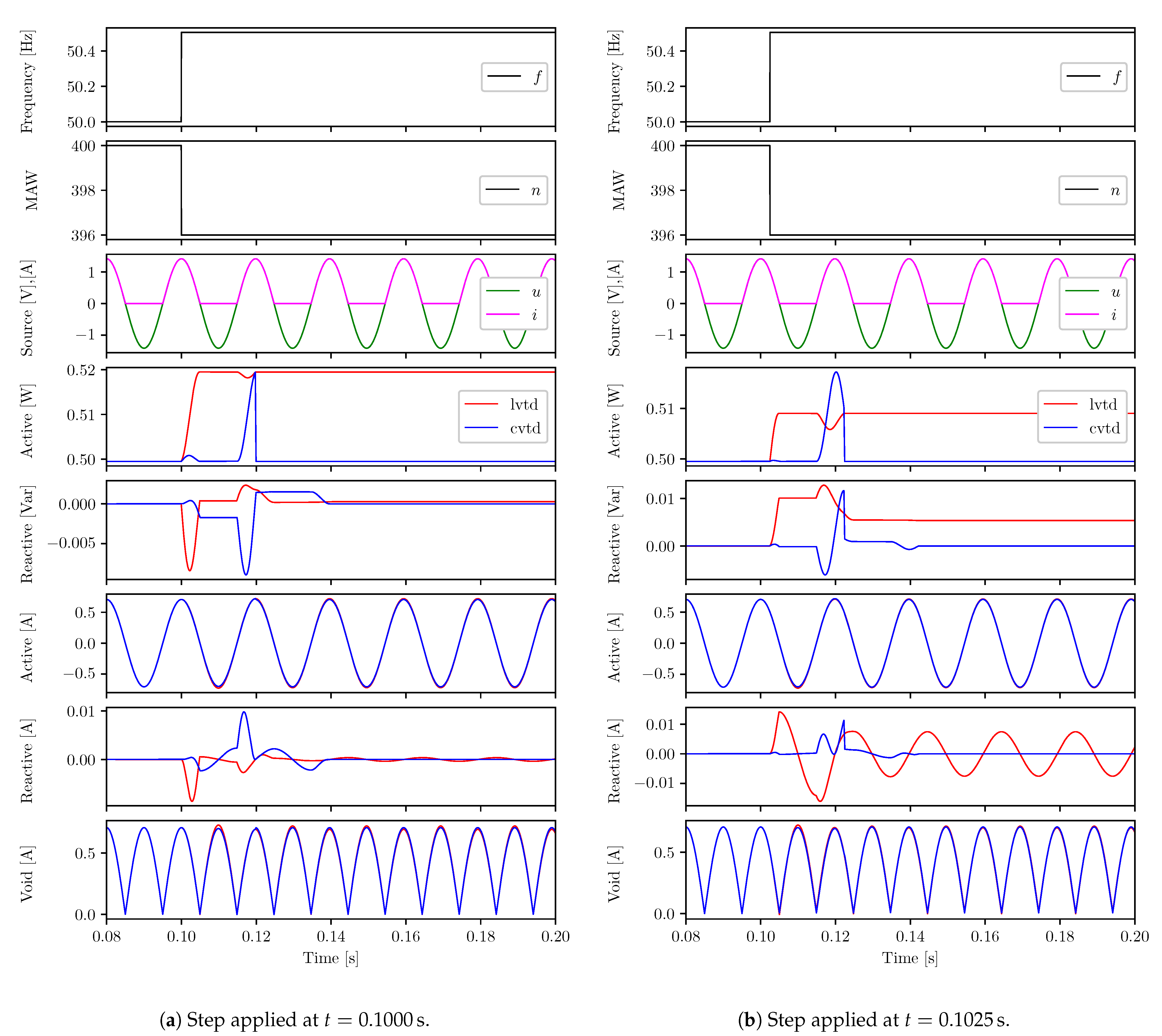
The positive steps applied are precisely calculated to decrease the MAWs from 400 to 396. Figure 7 shows the results of two positive steps applied at slightly different times for the DB-scenario. The measurements with LVTDs are in red. The measurements with CVTDs are in blue.

Frequency, MAW, and source voltage and current: in Figure 7a, the step is applied at the peak of the source voltage, $t=0.1\mathrm{s}$. In Figure 7b, the step in the frequency is applied $2.5\mathrm{m}\mathrm{s}$ after the peak of the voltage. The MAWs are updated immediately at the instants the frequency changes. Notice that the source current (magenta) is zero during the negative semi-cycle of the source voltage (green).

Active power: should be constant at $0.5\mathrm{W}$ irrespective of the frequency step. The retrieval pointers in the LVTDs jump over four slots when the MAW drops from 400 to 396. The values in these slots are not decumulated introducing a steady-state error in the active power. The error is on the range of 2% of a full scale of $1\mathrm{W}$ for the step at $t=0.1\mathrm{s}$. It is, however, approximately 1% for the step at $t=0.1025\mathrm{s}$. The measurements with CVTDs are auto corrected when the transient ends.

Reactive power: should be zero irrespective of the frequency step. The transient after the step lasts for two periods due to the cascaded AMAs. The measurements with CVTDs settle at the expected value after the transients. The steady-state errors introduced by LVTDs depend on which slots of the circular buffers are skipped. The error is barely noticeable in Figure 7a; however it is close to 0.5% of a full scale of $1\mathrm{Var}$ in Figure 7b.

Active current: neither the transients nor the steady-state measurement differences are noticeable in the curves at the scale shown.

Reactive current: is expected to be zero irrespective of the frequency variation. The error in the reactive current with LVTDs in Figure 7a is barely noticeable. This is a consequence of the small error in the reactive power for the step at instant $t=0.1\mathrm{s}$. On the other hand, the reactive current measured with LVTDs features a clear $50\mathrm{Hz}$ oscillation in Figure 7b. The measurements with CVTDs behave as expected.

Void current: the differences between the measurements from the CPT transducers with LVTDs and CVTDs are barely noticeable during the transient between $t=0.1\mathrm{s}$ and $t=0.14\mathrm{s}$.

9.1.3. Continuously Varying Frequency for Both Load Scenarios

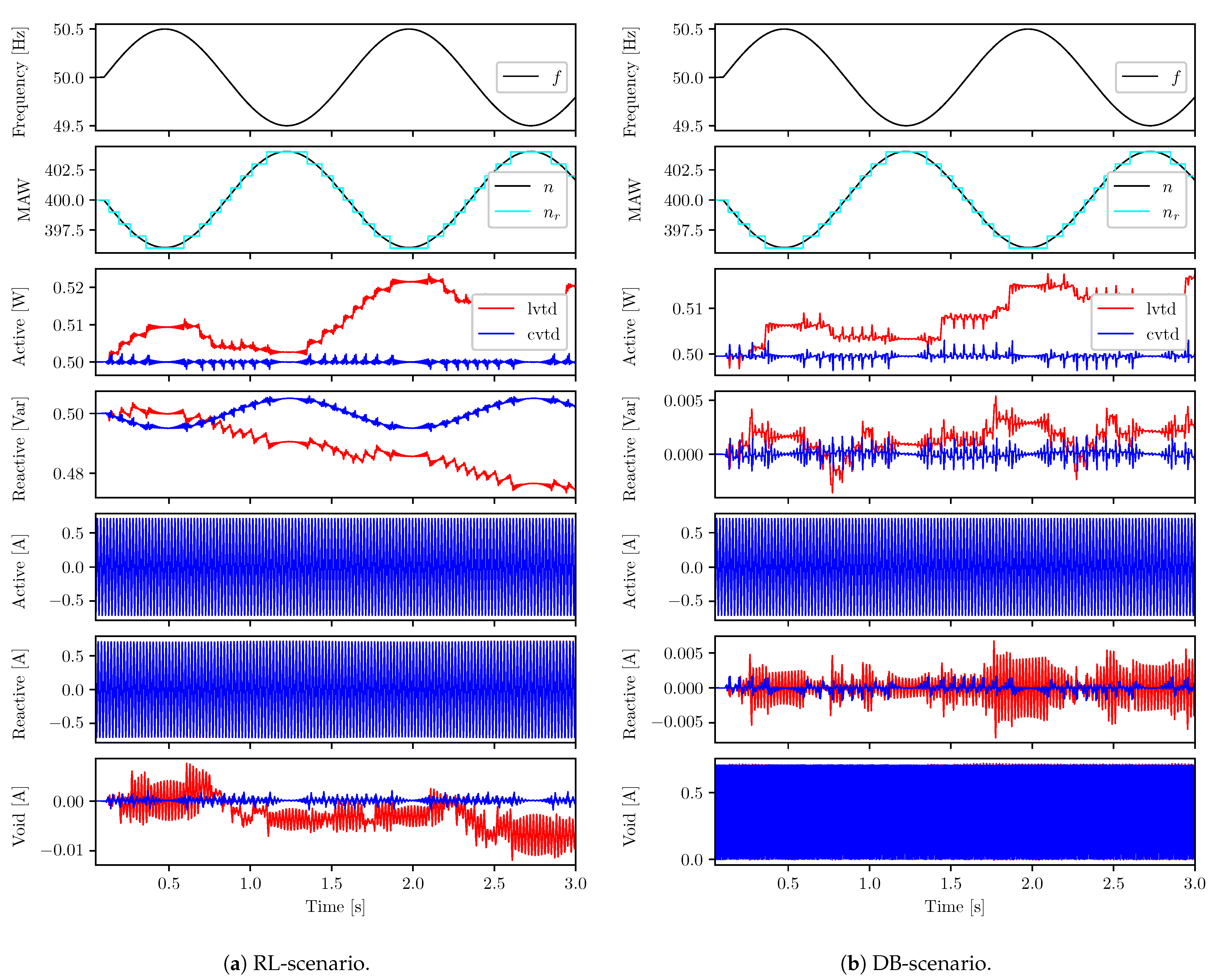
The steps used previously were purposefully calculated so the new value of $n_r{T}_s$ would be equal to the new period T. However, a more realistic test considers a continuous variation of the grid frequency, i.e., non-integer values of $n\left(k\right)$ from Equation (15). Figure 8 shows simulated measurements of two CPT transducers with either LVTDs (in red) or CVTDs (in blue) when the frequency of the voltage source varies in a sinusoidal form.

Frequency and MAW: a sinusoidal disturbance with amplitude of $0.5\mathrm{Hz}$ and frequency $2/3\mathrm{Hz}$ is summed to the rated value of the source frequency at instant $t=0.1\mathrm{s}$. The ideal value of the MAW n is shown in black. It goes down when the frequency increases and up when the frequency decreases. The rounded value of the MAW $n_r$ is shown in cyan.

Active power: should be constant at $0.5\mathrm{W}$ irrespective of the frequency changes. The randomness of the steady-state errors introduced by the LVTDs is especially noticeable in the DB-load scenario. Some changes in $n_r$ affect the active power measurement, some do not. The active power measured with the CVTDs does not feature noticeable steady-state errors. Nevertheless, the measurements with both LVTDs and CVTDs show transients lasting for $20\mathrm{m}\mathrm{s}$ after the MAW changes. Furthermore, a small $100\mathrm{Hz}$ oscillation is detected in the active power when $n_r$ differs from n in Figure 8a. Moreover, a $50\mathrm{Hz}$ pulsation is present in Figure 8b. Those are the natural pulsations of the instantaneous power, Equation (2), passing through the AMAs as previously commented in Section 6.

Reactive power: in the RL-scenario, the reactive power should vary inversely proportionally to the frequency. The measurement with CVTDs behaves as expected. However, the steady-state errors introduced by the LVTDs are clearly seen. In the DB-scenario, the reactive power should be zero irrespective of the frequency. The transducer with CVTDs behaves as expected, but the one with LVTDs does not.

Active current: the effects of the steady-state errors and transients are not large enough to be noticed in the active current in neither scenarios.

Reactive current: in the RL-scenario, the steady-state errors introduced in the reactive power do not cause noticeable errors in the reactive current. However, in the DB-scenario, they do.

Void current: in the DB-scenario, the steady-state errors introduced in the reactive power do not cause noticeable errors in the void current. However, in the RL-scenario, they do.

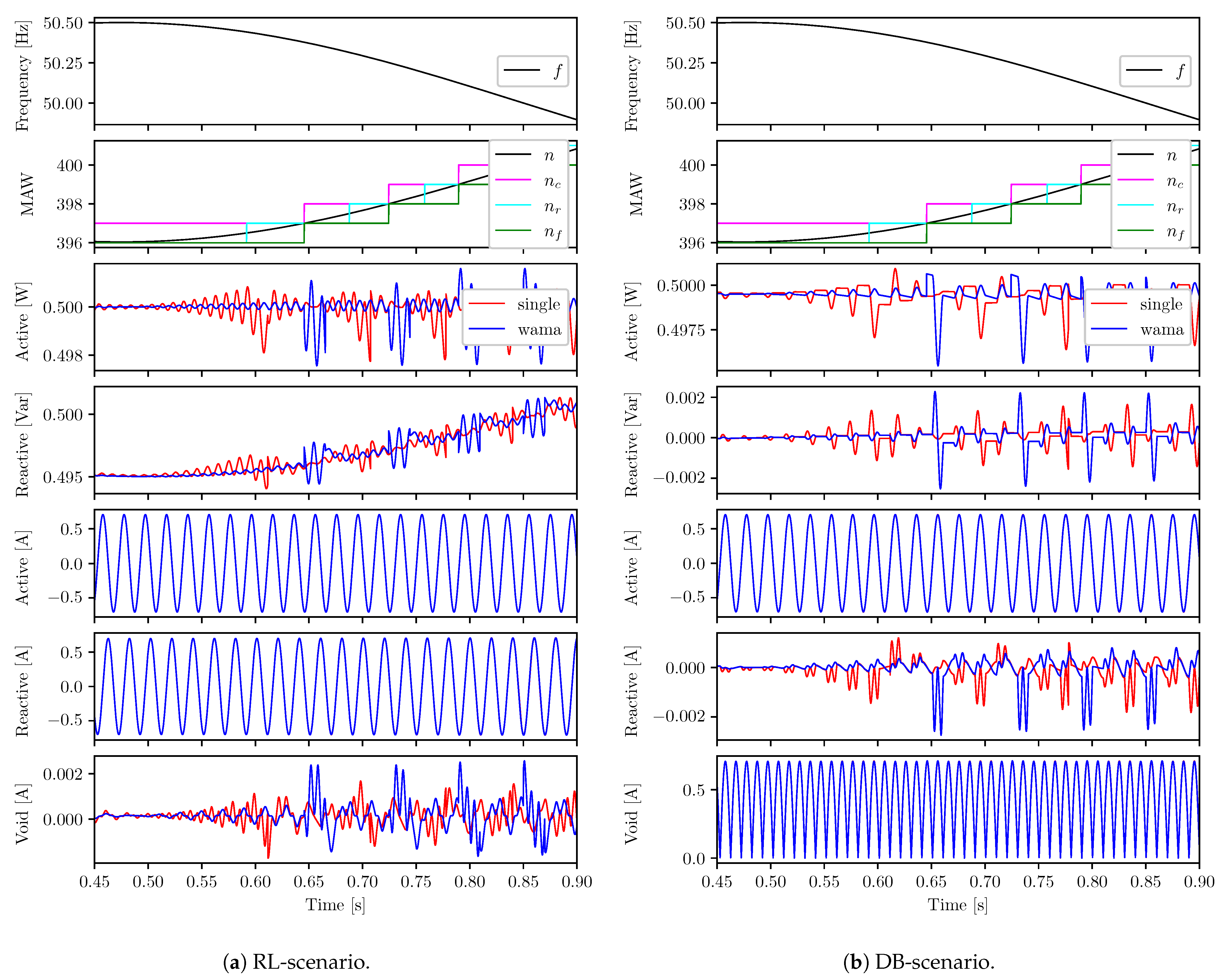
9.2. Single AMAs with Rounded MAWs versus WAMAs versus HAMA

Due to the poor performance seen in Section 9.1, LVTDs are not featured from here on. All results of the computer simulations shown from this point on were obtained with CPT transducers using exclusively CVTDs. For the sake of brevity, only the tests with a continuously variable grid frequency are presented.

9.2.1. Single AMA with Rounded MAW versus WAMAs

A disturbance with $0.5\mathrm{Hz}$ of amplitude and a frequency of $2/3\mathrm{Hz}$ is applied to the source voltage’s frequency at instant $t=0.1\mathrm{s}$ for both RL and DB-scenarios. Figure 9 shows a detail from $0.45$ to $0.90\mathrm{s}$ of the computer simulations. The measurements of the CPT transducer with single CVTDs with rounded MAWs are shown in red. The measurements with WAMAs are shown in blue.

Frequency and MAW: the frequency is at its peak at instant $t=0.45\mathrm{s}$. The ideal value of the MAW n is shown in black; it increases as the frequency drops. The ceiling ($n_c$ in magenta) and the floor ($n_f$ in green) values of the MAW are updated simultaneously when n crosses an integer value. Notice that the rounded value of the MAW ($n_r$ in cyan) does not change at the same time as $n_c$ and $n_f$ do.

Active power: the RL-scenario is shown in Figure 9a. The amplitude of the oscillations in the active power measured with single AMAs increases steadily as n drifts apart from $n_r$ after $t=0.45\mathrm{s}$. Just before $t=0.60\mathrm{s}$, $n_r$ is updated. This causes a $20\mathrm{m}\mathrm{s}$ transient in the red curve. Subsequently, the amplitude of the oscillations decreases and reaches a minimum when n is closest to $n_r$. The measurement with WAMAs features smaller oscillations up to instant $t=0.65\mathrm{s}$, when $n_c$ and $n_f$ change. However, the transients with WAMAs are worse than the ones with single AMAs. In the DB-scenario, the pulsating instantaneous power (not shown) is nonsinusoidal. It peaks at the positive semi-cycle of the source’s voltage and is zero during the negative semi-cycle. A parcel of those pulses slips through the single AMAs with rounded MAWs. The WAMAs, instead, are better at filtering the pulses.

Reactive power: similarly to the active power measurement, the WAMAs are better at filtering the pulsating instantaneous value of $w=\stackrel{⌢}{u}i\left(t\right)$ than the single AMAs. However, WAMAs feature worse transients when the MAW is updated.

Active current: the oscillations and transients are not noticeable in the curves at the scale shown.

Reactive current: in the RL-scenario, the differences between the measurements with single AMAs and WAMAs are not noticeable. The reactive current is expected to be zero in the DB-scenario. It is, therefore, easier to zoom in and show the differences. Up to instant $t=0.65\mathrm{s}$, the transducer with WAMAs performs better. Furthermore, similarly to the active power curves, the transients caused by the changes in $n_c$ and $n_f$ are worse in the CPT with WAMAs than the ones caused by the changes in $n_r$ for single AMAs.

Void current: in the DB-scenario in Figure 9b, the differences between the measurements with single ama and WAMAs are not noticeable. The void current is expected to be zero in the RL-scenario in Figure 9a. Up to instant $t=0.65\mathrm{s}$, the transducer with WAMAs performs better. However, the transients caused by the changes in $n_c$ and $n_f$ are worse in the CPT with WAMAs than the ones caused by the changes in $n_r$ for single AMAs.

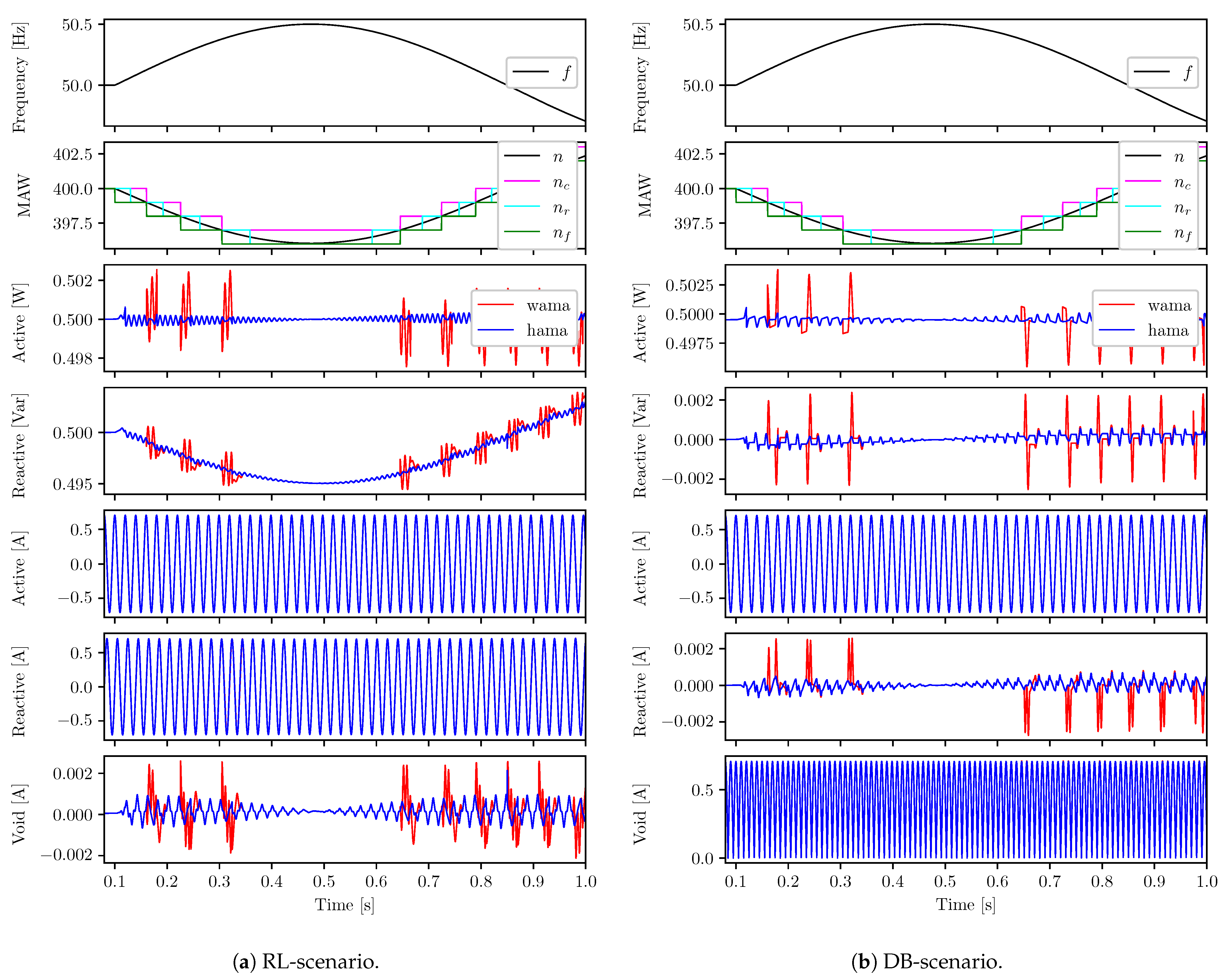
9.2.2. WAMA versus HAMA

In Figure 9, the transients of the single AMAs with rounded MAWs do not happen at the same time as the transients of the WAMAs. This inspired the creation of the HAMA which combines the output of a single AMA with rounded MAW and the output of one WAMA. It is worth mentioning, though, that this comes at the cost of extra memory.

Figure 10 shows the results of the computer simulations comparing the measurements of two CPT transducers. The transducer with WAMAs is shown in red. The one with HAMAs is shown in blue.

Frequency and MAW: the disturbance at the frequency of the voltage source starts at $t=0.1\mathrm{s}$. The frequency of the disturbance is $2/3\mathrm{Hz}$. The ideal value of the MAW n is shown in black; it reacts instantaneously to the changes in the frequency. The ceiling ($n_c$ in magenta) and the floor ($n_f$ in green) values of the MAW are updated simultaneously when n crosses an integer value.

Active power: a HAMA incorporates one single AMA with rounded MAW and one WAMA. By choosing to output ${\overline{x}}_r$ for one period of the grid after $n_c$ and $n_f$ change, refer to Section 7, the HAMAs remove the transients observed in the active power measured with WAMAs.

Reactive power: similarly to the active power measurement, the HAMAs remove the unwanted transient from the measurements with WAMAs. It is interesting to remark that the strategy of switching ${\overline{x}}_w$ by ${\overline{x}}_r$ for only one period of the grid, see Section 7, works well despite the two-period transients in the reactive power measurements caused by cascaded AMAs.

Active current: the oscillations and transients in the active current are not noticeable at the scale the curves are presented.

Reactive current: in the RL-scenario, the differences between the measurements with WAMAs and HAMAs are not noticeable. The reactive current is expected to be zero in the DB-scenario. It is, therefore, easier to zoom in and highlight the differences between WAMAs and HAMAs. The measurement with HAMAs does not feature the transients observed in the measurement with WAMAs.

Void current: the void current is expected to be zero in the RL-scenario. The HAMAs effectively remove the transients observed in the measurement with WAMAs. In the DB-scenario, the differences between the measurements with WAMAs and HAMAs are not noticeable.

10. Conclusions

In the modern smart-grid scenario characterized by an increasing participation of renewable energy sources, energy storage devices, and smart load management systems, the CPT emerged as a theoretical framework for coping with harmonically distorted and unbalanced electric networks. Isolated grids with reduced inertia, microgrids included, may experience large frequency variations. The application of the CPT for the compensation of harmonic distortions and unbalances in such grids is predicated on the appropriate measurement of the CPT’s basic electrical quantities. Those measurements, which are intrinsically linked to AMAs, need to be correct not only in steady state, but during unexpected excursions of the grid frequency as well.

A computational efficient way of calculating MAs is briefly reviewed with a discussion on how to turn it into an adaptive one in Section 4. The concepts of accumulation and decumulation are presented emphasizing their importance in the calculation of a correct AMA. Moreover, an AMA needs a VTD block. Two different ways of implementing a VTD are presented in Section 4.1 and Section 4.2, the LVTD and the CVTD, respectively. Two CPT transducers based on AMAs with either LVTDs or CVTDs are tested through computer simulations in Section 9.1 with the following results.

• The LVTD, which is readily available from [11], introduces noticeable steady-state errors in the active and reactive power measurements when the frequency changes and the MAW is updated. Furthermore, errors in the reactive current are noticeable for the case of a nonlinear load, whereas errors in the void current are noticeable for the case of a linear load.
• The CVTD, which is proposed in this paper, is easily programmable and demands the same amount of memory as the LVTD. The CVTD auto corrects the measurements after changes to the MAW. However, similarly to the LVTD, it causes transients lasting one grid period in the active power and active current measurements after changes to the MAW. The transients in the measurements of the reactive power and the reactive and void currents last for two grid periods.

Both CPT transducers built with either LVTDs or CVTDs let through a noticeable parcel of the instantaneous pulsations in $p=ui$ and $w=\stackrel{⌢}{u}i$ when the ideal value of the MAW is different from the rounded one. This comes from the impossibility of matching perfectly the integer $n_r$ , Equation (16), with the continuously varying real number n, Equation (15). Nevertheless, the main conclusion from the results of Section 9.1 is: the readily available LVTD should not be used in AMAs built as in Figure 1, the newly proposed CVTD should be used instead.

A weighting of MAs proposed by [15] for tackling the problems related to rounding the MAW is briefly reviewed in Section 6. This method is named WAMA in this paper. An improvement of the WAMA is proposed in Section 7 and is called HAMA. Three CPT transducers based on single AMAs with rounded MAWs, on WAMAs, and on HAMAs are compared via computer simulations in Section 9.2. The results are summarized below.

• The WAMA is better than a single AMA with rounded MAW at filtering the pulsations in $p=ui$ and $w=\stackrel{⌢}{u}i$ as shown in Section 9.2.1. However, the WAMA features noticeable transients when the ceiling and floor values of the MAW are updated. The amplitude of those transients is larger than both the oscillations and the transients observed in the measurements with single AMAs with rounded MAWs. This, summed to its extra demand in memory, places the WAMA behind the single AMA with rounded MAW in a ranking of best AMA methods for implementing the CPT in systems with variable frequency.
• The HAMAs efficiently remove the transients observed in the measurements with WAMAs as shown in Section 9.2.2. This comes at a cost of 50% more memory usage when compared to WAMAs. Despite that, the HAMA ranks best among the AMA methods analyzed in this paper.

Table 3. Assessment of three CPT transducers using either single AMAs with rounded MAWs, WAMAs, or HAMAs.

Criteria	Single AMAs	WAMAs	HAMAs
Blocking natural pulsations of p and w	worst	good	best
Transients when updating the MAWs	bad	worst	best
Memory usage	best	bad	worst

compares three single-phase CPT transducers built according to Figure 3 and Figure 4, running with a sampling frequency as defined in Table 1, and using either single AMAs with rounded MAWs, WAMAs, or HAMAs. It is worth stressing that due to the poor performance of the AMAs with LVTDs, only CVTDs were employed in the transducers shown in Table 3.

The frequency measurement was assumed to be instantaneous and without noise throughout the whole paper. The MAWs were, thus, updated instantaneously. In a future research, the authors wish to investigate the effects of nonideal frequency measurements in the performance of the CPT transducers with different choices of AMAs.

Even though the CPT applied to isolated ac grids with variable frequency was used as backdrop, the authors believe that the discussions and new methods proposed in this article show higher generality and are applicable to other fields which employ AMAs.

References

- Tenti, P.; Mattavelli, P. A Time-Domain Approach to Power Term Definitions under Non-Sinusoidal Conditions. L’Energia Elettr. 2004, 81, 75–84. [Google Scholar]
- Busarello, T.D.C.; Pomilio, J.A.; Simões, M.G. Passive Filter Aided by Shunt Compensators Based on the Conservative Power Theory. IEEE Trans. Ind. Appl. 2016, 52, 3340–3347. [Google Scholar] [CrossRef]
- Mortezaei, A.; Simões, M.G.; Busarello, T.D.C.; Marafão, F.P.; Al-Durra, A. Grid-Connected Symmetrical Cascaded Multilevel Converter for Power Quality Improvement. IEEE Trans. Ind. Appl. 2018, 54, 2792–2805. [Google Scholar] [CrossRef]
- Alonso, A.M.S.; Paredes, H.K.M.; Filho, J.A.O.; Bonaldo, J.P.; Brandão, D.I.; Marafão, F.P. Selective Power Conditioning in Two-Phase Three-Wire Systems Based on the Conservative Power Theory. In Proceedings of the 2019 IEEE Industry Applications Society Annual Meeting, Baltimore, MD, USA, 29 September–3 October 2019; pp. 1–6, ISSN 2576-702X. [Google Scholar] [CrossRef]
- Tedeschi, E.; Tenti, P. Cooperative design and control of distributed harmonic and reactive compensators. In Proceedings of the 2008 International School on Nonsinusoidal Currents and Compensation, Lagow, Poland, 10–13 June 2008; pp. 1–6, ISSN 2375-1428. [Google Scholar] [CrossRef]
- Tenti, P.; Mattavelli, P.; Morales Paredes, H.K. Conservative Power Theory, sequence components and accountability in smart grids. In Proceedings of the 2010 International School on Nonsinusoidal Currents and Compensation, Lagow, Poland, 5–18 June 2010; pp. 37–45, ISSN 2375-1428. [Google Scholar] [CrossRef]
- Tenti, P.; Paredes, H.K.M.; Mattavelli, P. Conservative Power Theory, a Framework to Approach Control and Accountability Issues in Smart Microgrids. IEEE Trans. Power Electron. 2011, 26, 664–673. [Google Scholar] [CrossRef]
- Czarnecki, L.S. Critical comments on the Conservative Power Theory (CPT). In Proceedings of the 2015 International School on Nonsinusoidal Currents and Compensation (ISNCC), Lagow, Poland, 15–18 June 2015; pp. 1–7, ISSN 2375-1428. [Google Scholar] [CrossRef]
- Orfanidis, S.J. Introduction to Signal Processing; Prentice Hall, Inc.: Upper Saddle River, NJ, USA, 1996; ISBN 0-13-209172-0. [Google Scholar]
- Golestan, S.; Ramezani, M.; Guerrero, J.M.; Freijedo, F.D.; Monfared, M. Moving Average Filter Based Phase-Locked Loops: Performance Analysis and Design Guidelines. IEEE Trans. Power Electron. 2014, 29, 2750–2763. [Google Scholar] [CrossRef]
- MathWorks Documentation Archive—Matlab Simulink R2018a—Delay Input Signal by Fixed or Variable Sample Periods. Available online: https://mathworks.com/help/releases/R2018a/simulink/slref/delay.html?searchHighlight=delay&s_tid=doc_srchtitle (accessed on 23 October 2020).
- Comanescu, M. Influence of the discretization method on the integration accuracy of observers with continuous feedback. In Proceedings of the 2011 IEEE International Symposium on Industrial Electronics, Gdansk, Poland, 27–30 June 2011; pp. 625–630, ISSN 2163-5145. [Google Scholar] [CrossRef]
- Lyons, R.G. Understanding Digital Signal Processing; Prentice Hall PTR: Upper Saddle River, NJ, USA, 2001; ISBN 0-201-63467-8. [Google Scholar]
- Ama, N.; Destro, R.; Komatsu, W.; Kassab, F.; Matakas, L. PLL performance under frequency fluctuation-compliance with standards for distributed generation connected to the grid. In Proceedings of the 2013 IEEE PES Conference on Innovative Smart Grid Technologies (ISGT Latin America), Sao Paulo, Brazil, 15–17 April 2013; pp. 1–6. [Google Scholar] [CrossRef]
- Svensson, J.; Bongiorno, M.; Sannino, A. Practical Implementation of Delayed Signal Cancellation Method for Phase-Sequence Separation. IEEE Trans. Power Deliv. 2007, 22, 18–26. [Google Scholar] [CrossRef]
- Bonaldo, J.P.; Paredes, H.K.M.; Pomilio, J.A. Control of Single-Phase Power Converters Connected to Low-Voltage Distorted Power Systems With Variable Compensation Objectives. IEEE Trans. Power Electron. 2016, 31, 2039–2052. [Google Scholar] [CrossRef]
- Brandao, D.I.; Guillardi, H.; Morales-Paredes, H.K.; Marafão, F.P.; Pomilio, J.A. Optimized Compensation of Unwanted Current Terms by AC Power Converters Under Generic Voltage Conditions. IEEE Trans. Ind. Electron. 2016, 63, 7743–7753. [Google Scholar] [CrossRef]