Article

Comparative Analysis of Machine Learning Models for Day-Ahead Photovoltaic Power Production Forecasting †

by
Spyros Theocharides
1,*,
Marios Theristis
2,
George Makrides
1,
Marios Kynigos
1,
Chrysovalantis Spanias
3 and
George E. Georghiou
1
1
PV Technology Laboratory, FOSS Research Centre for Sustainable Energy, Department of Electrical and Computer Engineering, University of Cyprus, Nicosia 1678, Cyprus
2
Sandia National Laboratories, Albuquerque, NM 87185, USA
3
Distribution System Operator, Electricity Authority of Cyprus (EAC), Nicosia 1399, Cyprus
*
Author to whom correspondence should be addressed.
This paper is an extended version of our paper published in 2018 IEEE International Energy Conference (ENERGYCON) Conference, Limassol, Cyprus, 3–7 June 2018; pp. 1–6.
Energies 2021, 14(4), 1081; https://doi.org/10.3390/en14041081
Submission received: 27 January 2021 / Revised: 13 February 2021 / Accepted: 16 February 2021 / Published: 18 February 2021
(This article belongs to the Special Issue Smart Photovoltaic Energy Systems for a Sustainable Future)

Abstract

:
A main challenge for integrating the intermittent photovoltaic (PV) power generation remains the accuracy of day-ahead forecasts and the establishment of robust performing methods. The purpose of this work is to address these technological challenges by evaluating the day-ahead PV production forecasting performance of different machine learning models under different supervised learning regimes and minimal input features. Specifically, the day-ahead forecasting capability of Bayesian neural network (BNN), support vector regression (SVR), and regression tree (RT) models was investigated by employing the same dataset for training and performance verification, thus enabling a valid comparison. The training regime analysis demonstrated that the performance of the investigated models was strongly dependent on the timeframe of the train set, training data sequence, and application of irradiance condition filters. Furthermore, accurate results were obtained utilizing only the measured power output and other calculated parameters for training. Consequently, useful information is provided for establishing a robust day-ahead forecasting methodology that utilizes calculated input parameters and an optimal supervised learning approach. Finally, the obtained results demonstrated that the optimally constructed BNN outperformed all other machine learning models achieving forecasting accuracies lower than 5%.

1. Introduction

The world is entering a new era with photovoltaic (PV) technologies emerging as the primary source for meeting future electricity demands, while coal-fired generation declines globally [1]. Driven by cost reductions and concerted government policy efforts, the world’s total renewable-based power capacity is expected to grow by 50% over the coming years with PV accounting for 60% of this rise [2]. The integration of higher shares of variable renewable energy (VRE) technologies, such as PV, is essential for decarbonizing and meeting the demands of future grids but introduces new grid operation challenges. In particular, the increasing deployment of VRE generation poses specific challenges as its share of power generation rises, rendering new power system flexibility options critical for ensuring continuous service in the face of rapid and large swings in supply or demand (real-time operations to long-term system planning) [3].
In this domain, the variability and uncertainty of PV generation incurs serious stability and reliability issues in power system operations since the intermittent nature of solar produced electricity must be accommodated by grid operators in their generation planning and dispatch operations [4,5,6]. Utility grids with large share deployment of distributed PV systems are already experiencing a profound transformation towards modern digitally enhanced technologies that will enable the observability and control of underlying distributed energy resources (DERs). To this end, the current electrification, decentralization, and digitalization trends are accelerating the transformation of the existing power sector paradigm in order to fully unlock system flexibility for high VRE penetration.
To stem grid transition and mitigate adverse power quality impacts posed by high shares of PV systems, utilities require PV power forecasts for core generation dispatch and scheduling operations. Forecasting is a main enabler that can ensure secure and economic integration of PV while building links for synergies between many flexibility innovations in power systems across different dimensions. Forecasts focus on the output power or the rate of change of power (ramp rate) of a single PV system or the aggregation of large numbers of systems. More specifically, accurate PV power forecasting is an important cost-effective energy management element for utilities and plant operators that can save excessive spinning reserve, enhance the stability of the system, reduce integration and ancillary services costs, and ensure seamless integration of VRE sources. Furthermore, it allows the efficient and direct participation of PV power plants and aggregated systems into electricity markets by optimizing schedules for the supply and increasing revenues. Incidentally, forecasting provides the necessary tool for distribution areas to become commercially viable microgrids and to be aggregated in virtual power plants (VPPs) in order to spur the value of low-cost solar electricity.
Over the past years, a large number of forecasting methods have been presented in the literature to address this challenge. In general, forecasting methods are categorized according to the forecasting time horizon (i.e., the amount of time between the actual effective prediction time), the approach to yield the forecasts and the particular application of the forecasted outputs [7]. Regarding the various forecasting horizon methods, these can be further classified into very short-term, short-term, medium-term, and long-term forecasting [8,9,10]. In particular, the forecast horizons of medium-term and long-term forecasting methods typically range from 1 month to 1 year and 1–10 years, respectively [10]. These forecasting approaches are mainly applied for scheduling and planning in the power sector. On the other hand, very short-term forecasting methods cover horizons of 1 min to 1 h and are applied in real-time operations (i.e., automatic generation control, power smoothing, real-time power dispatching, and spot markets). Accordingly, short-term forecasts typically range from 1 h to 1 week and are required in unit commitment, economic dispatching, reserve optimization, storage system management, transmission scheduling, and day-ahead markets. For very short-term forecasting, onsite PV system measurements and meteorological data are necessary, while numerical weather prediction (NWP) datasets are commonly utilized for forecasts extending beyond 6 h. Both very short- and short-term forecasts are also defined as intraday, and at the present day-ahead forecasting of the hourly output power, it is the most important component for the integration of PV in electric grids [9].
In contrast to the very short-term PV generation forecasting methods that rely on historical observations and statistical approaches to train models, day-ahead forecasts require weather forecasts from NWP models as the key inputs to PV power prediction models that generate forecasts [9]. More specifically, NWP models are based on dynamical equations that describe the evolution of atmospheric physical processes and are classified as either global or mesoscale. Global models such as the global forecast system (GFS) [11], have a global coverage with spatial resolution of around 1° (approximately 100 km at the earth’s surface). Mesoscale models usually include topographic details and information at different levels from the ground level up to the stratosphere. One of the main outputs of NWP models for solar forecasting is the global horizontal irradiance (GHI) at the ground level. Previous studies focused on improving the accuracy of GHI recasts by employing spatial averaging and bias removal techniques [12,13,14,15,16,17]. The most commonly employed mesoscale NWP model is the weather research and forecasting (WRF), which is designed for both atmospheric research and operational forecasting applications [18]. Ongoing energy meteorology research efforts focus on the configuration and adaptation of WRF models for solar-specific applications, as in the case of WRF-Solar [19].
In day-ahead PV power production forecasting the NWP forecasts (solar irradiance and temperature) are applied directly to PV performance predictive models to yield the power output of a PV plant. Aided by internet of things (IoT) and high-speed computing evolution, recent advances involve more sophisticated predictive models that utilize data-driven approaches based on machine learning (ML) principles in order to gain insight on large amounts of data to uncover hidden patterns. The application of ML predictive models is continuously gaining ground in the renewable sector due to their improved accuracy and robustness over other modelling approaches. Furthermore, these predictive models form the basis of digital twin technologies, which are virtual system that replicate the operation of a PV system and are useful for both proactive and reactive performance analytics. In addition, with data-driven approaches the technical barriers such as the lack of PV system characteristics information and operational performance status are overcome [20,21,22,23,24,25,26,27,28,29,30]. This is essential since a large share of PV systems are decentralized behind the meter (BTM) and system metadata (plant location, geometry, nearby obstructions, and hardware information) are rarely available. Most commonly applied supervised learning approaches for PV generation forecasting include support vector machines (SVMs) [31,32,33], artificial neural networks (ANNs) [34,35,36], random forests (RF) [37,38], and other deep learning methods [39,40,41,42,43].
Even though there is a multitude of employed techniques, a unified data-driven methodology that yields accurate PV production forecasts over various time scales is desirable but challenging for future smart grid applications. A study by the California Renewable Energy Collaborative (CREC) showed that accurate day-ahead PV generation forecasts of up to 6% root mean square error (RMSE) are obtained only for clear sky days [44]. Under other sky conditions nRMSE values of at least 20% were obtained, even though several occurrences in the range of 40–80% were observed [44]. Another study proposed the application of different types of ANNs that yielded forecasting errors in the range of 15.2% to 16.3% for the next day [26]. Similarly, an adaptive feed-forward back-propagation network (AFFNN) for short-term forecasting was applied providing a mean absolute percentage error (MAPE) lower than 5% for sunny days [23]. According to many authors and reviews, ANN-based forecasting techniques prove to be very effective due to their inherent ability to capture non-linear abrupt changes caused by the varying environmental conditions between the input–output relationship [23,26,45,46].
Along this context, the performance comparison of different techniques applied for day-ahead forecasting is a challenging task since numerous factors influence the performance such as the availability of historical data and weather forecasts, the temporal horizon and resolution, the weather conditions, the geographical location, and the installation conditions [47]. Apart from the use of conventional data-driven ML techniques, prior studies focused in utilizing hybrid models, in an attempt to improve the forecasting accuracy by merging features of physical models to ML techniques [47,48,49]. In particular, a previous study employing a self-organizing map that classified the weather type in the training stage of an ANN model achieved MAPE of 6.36% [48]. Another investigation demonstrated that the application of a physical hybrid artificial neural network (PHANN) for clear sky days provided a normalized mean absolute percentage error (NMAE) of 5.3% [47].
Even though there are many studies presenting day-ahead PV production methods based on data-driven techniques, the lack of a widely recognized practice and standardized procedure to accurately yield forecasts for PV systems beyond the state-of-the-art, remains yet an important challenge. In addition, the question related to the impact of different supervised learning regimes (effect of training period, training data sequence, and application of irradiance condition filters) is yet unexplored and necessary for more reliable forecasts that will further increase the potential of PV and lead to industrial standards. To this end, research efforts are further striving to develop accurate data-driven forecasting models that are based on minimal measured parameters.
The main aim of this work is to present a robust day-ahead PV production forecasting methodology and fill-in the gap of knowledge by evaluating the forecasting accuracy of different supervised trainings. For this purpose, a comparative analysis of widely used ML techniques that leverage Bayesian neural network (BNN), support vector regression (SVR), and regression tree (RT) principles was performed in order to evaluate their effectiveness for PV power forecasting applications. The proposed methodology included training the different ML PV predictive models (digital twins that were thoroughly investigated by Theocharides et al. [43]), under different supervised learning regimes and benchmarking the forecasting performance. The verification was carried out using actual high-quality hourly PV operational and meteorological measurements acquired over a period of two years from a test-bench PV system installed at the outdoor test facility (OTF) of the University of Cyprus (UCY) in Nicosia, Cyprus. Alongside the on-site measurements, NWP hourly data were computed at a spatial resolution of 2 × 2 km for the point location of the test-bench PV system. The test-bench PV system settings provide the perfect opportunity to study the effect of the supervised training regimes to the forecasts based on commonly used metrics. Furthermore, the forecasting accuracy of the constructed models was compared against a baseline persistence model (PM) in order to assess the effectiveness of each machine learning technique. The analysis verified the initial hypothesis that the choice of the predictive model and training regime are crucial for the forecasting accuracy. Additionally, the obtained results provided useful information for the establishment of a robust day-ahead forecasting methodology that utilizes only computed input parameters and an optimal supervised learning approach.

2. Materials and Methods

The methodology followed to develop the day-ahead PV production forecasting models and to evaluate the impact of different supervised learning regimes included the experimental setup, construction of the optimal performing predictive PV power output ML models, and the performance verification using consistent metrics applied to the same dataset. The proposed method is illustrated in Figure 1. In this study, the ML techniques of BNNs, SVR, and RTs were used for predicting the power output. These models were selected amongst a list of candidate ML models (e.g., ANN, BNN, SVR, long short-term memory [LSTM], recursive neural networks [RNN], RT, etc.), based on their accuracy performance on similar applications, computing complexity, execution time for training, dataset pipeline, and ease of hyperparameter management [41,42]. Regarding the selection of the model based on neural networks, the BNN was used in contrast to other already investigated approaches such as the LSTM and RNNs [41,42,43,44,45,46,47,48], mainly to prove that higher forecasting accuracies can be achieved using stochastic optimization approaches even at low dataset sizes and at high-varying environments.
In respect to the construction and optimization process of the ML-based models:
  • The BNN, SVR, and RT models were trained with the same input features (input range, sampling rate, and parameters);
  • The trained models were used to optimize their hyperparameters over a series of empirical and statistical procedures;
  • The optimized models were verified through a series of performance evaluation techniques.
Figure 1 demonstrates the aforementioned methodology.

2.1. Experimental Setup

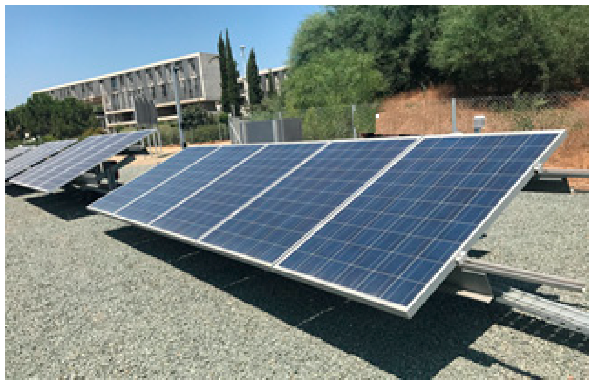
The OTF at the UCY in Nicosia, Cyprus (Koppen’s classification BSh; hot semi-arid) is a flexible and scalable testing, demonstration, and R&D platform for smart grid and other advanced energy technologies. In addition, the infrastructure includes, among others, a test-bench grid-connected PV system used for the forecasting analysis of this study, as shown in Figure 2. The test-bench PV system comprises of 5 polycrystalline silicon (poly-c Si) PV modules of rated power 235 Wp that are installed in an open-field arrangement at an inclination angle of 27.5°. The modules are connected in series to form a string of nominal capacity 1.175 kWp at the input of a grid-connected inverter. The infrastructure is further equipped with a state-of-the-art weather station and meteorological datasets are continuously acquired and analyzed in order to facilitate research in the area of energy meteorology and PV production forecasting.
The performance of the test-bench PV system and the prevailing weather conditions were recorded and stored with the use of a data acquisition (DAQ) monitoring platform according to the requirements set by the International Electrotechnical Commission (IEC) 61724 [50]. The measured meteorological parameters included the in-plane solar irradiance ( G I ), wind direction ( W a ), wind speed ( W s ), as well as ambient temperature ( T amb ).The PV system operational measurements included the maximum power point (MPP) current ( I mp ), voltage ( V mp ), and power ( P mp ), as measured at the output of the PV array (DC side) and module temperature ( T mod ). AC energy measurements at the output of the inverter were also acquired using an energy meter. The Sun’s position parameters (i.e., solar azimuth ( φ s ) and elevation ( α ) angles) were calculated using solar position algorithms [51]. The system was continuously monitored and high-quality data (at a resolution of a second and recording interval of 1-, 15-, 30-, and 60-min) were acquired over a 2-year period. All the installed sensors and the associated measurement accuracies (acquired from manufacturer datasheets and calibration files) are summarized in Table 1.
The system and pyranometer were cleaned on a seasonal basis and after dust events in order to minimize any soiling effects. Systematic recalibration of the sensors was performed as specified by the manufacturers and periodic cross-checks against neighboring sensors (other pyranometers and temperature sensors installed in close proximity) were conducted in order to identify sensor drifts.
In addition, NWP data were computed by the Department of Meteorology of Cyprus at a spatial resolution of 2 × 2 km for the point location of the test-bench PV system. More specifically, the two-year numerical forecast dataset was derived by employing the WRF 3.6.1 model with two-way nesting. The forecasted NWP dataset comprised of the hourly points of the forecasted G H I ( G H I _ F ), T amb ( T amb _ F ), W a ( W a _ F ), W s ( W s _ F ) , cloud index ( C I _ F ) and relative humidity ( R H _ F ). The numerical forecast dataset of the 1st year was employed to train the machine learning predictive models while the dataset of the 2nd year was used as a test set for forecasting performance verification.
In this study, the high-quality datasets acquired from the test-bench PV system were used for constructing the predictive machine learning models and for validating their performance accuracy under different training regimes. In particular, a 2-year dataset with hourly measurements of G I , T amb and P mp was constructed and merged with the forecasted NWP hourly dataset.
Initially, the acquired measurements were thoroughly inspected for erroneous values, outliers, gaps, and repetitions similar to a process presented by Livera et al. [52]. Sequential steps of filtering and data mining inference routines were applied to the dataset in order to ensure data fidelity before proceeding with the data-driven approaches. The specific data mining techniques were applied to detect features that differ significantly from normal instances by setting threshold ranges for the acquired measurements, missing data by searching for not available (NA) values, and repetitive measurements. All detected erroneous and missing data were discarded from the initial dataset.
The day-ahead PV production forecasting models and statistical data analytics were performed using the R Statistical Language [53], which is a free open-source environment for statistical computing and graphics development. The R tool also provides a variety of basic built-in libraries that were used and adjusted in order to develop customized software scripts for supervised learning approaches and performance benchmarking. Finally, the NWP data were derived using the WRF 3.6.1 model [18].

2.2. PV Power Output Predictive Models

The analysis in this paper is a continuation of a prior research on the construction of PV power output machine learning predictive models with optimal input features [43], by evaluating the day-ahead forecasting performance of models based on BNN, SVR, and RT techniques under different training algorithms (training with measured or computed input variables, training sequentially or randomly with values of different timeframes, and training with filtered irradiance data).
The 2-year evaluation dataset was separated into the train and test sets using different data split approaches. More specifically, 10 different train sets were extracted from the original time series by partitioning the 1st year evaluation dataset sequentially or randomly into portions of 10%, 30%, 50%, and 70%. Additionally, in order to assess whether an entire year is required for accurate forecasting a train set comprising of the data of the entire 1st year was also used. Previous work by [54] showed that machine learning models with input feature combinations of measured or forecasted irradiance, temperature, and the Sun’s position angles outperformed any other input parameter selection. For the purpose of this work and to demonstrate whether accurate forecasts can be obtained using only computed input values or not, each train set included the input features of the on-site measured G I and T amb , calculated φ s and α , forecasted G H I _ F and T amb _ F , and the output variable of P mp . The constructed train and test set partitions and included features are summarized in Table 2. In all cases, the entire 2nd year of the evaluation dataset was used as the test set in order to provide a common benchmarking dataset that accounted for all seasonality that may exhibited throughout the year.
To further evaluate the effect of training the machine learning forecasting models at low and high irradiance conditions, an irradiance filter was applied to the 1st year evaluation period train set. The applied filters included a low-pass filter that filtered out high irradiance conditions of irradiance levels >600 W/m2 (i.e., kept low and moderate irradiance conditions) and a high-pass filter that filtered out data at irradiance levels ≤600 W/m2 (i.e., kept high irradiance conditions). Subsequently, both the low- and high-irradiance datasets were used to train the different machine learning models (BNN, SVR, and RT).
Finally, for each constructed day-ahead PV forecasting model, additional hyper-parameter optimization steps were performed to ensure that for each technique the optimal models were selected. Specifically, the number of hidden units and epochs for the BNN were varied by performing an automated grid search for the cost of constraints and the scaling parameter ( γ ) in the case of SVR and optimizing the complexity parameter (CP) of the RT model (more details in Section 2.2.1, Section 2.2.2 and Section 2.2.3).

2.2.1. Bayesian Neural Networks

Even though deep learning approaches such as deep neural networks (DNNs) proved to be robust to natural variations and flexible in being applied to different applications and data types, these models are prone to overfitting and tend to be overconfident about their predictions. This adversely affects the generalization capabilities of the constructed models. Consequently, an approach to improve the generalization capabilities of the constructed models is to use stochastic neural networks that are able to estimate the prediction uncertainty. In this domain, the Bayesian paradigm provides the framework to analyze and train neural networks stochastically and to quantify the uncertainty associated with the predictions [55]. It also gives a mathematical framework to understand many regularization techniques and learning strategies that are already used in classic deep learning [56].
In general, the training of ANNs is performed by minimizing a cost function with the error term referring to the discrepancy between the predicted and actual output. The error is commonly measured using the mean square error (MSE) and error minimization is achieved with the back-propagation (BP) algorithm. The BP algorithm calculates the error contribution of each neuron after a batch of data by distributing the error back from the output through the network layers. In addition, the cost function is often associated with a regularization term to penalize parametrizations and control the complexity of the network.
Conversely, a BNN is a type of ANN that is constructed by introducing stochastic components into the network architecture (activation and weights) to simulate multiple possible models with an associated probability distribution. To this end, BNNs are considered to be a special case of ensemble learning, where instead of training one single model, a set of models is trained, and their predictions are aggregated [57]. The Bayesian paradigm is based on the principle that probability is a measure of belief in the occurrence of events and that prior beliefs influence posterior beliefs. Once the data were fitted, the density function for the weights was updated according to Bayes’ rule [22,58]:
P ( w | D , α , β , Μ ) = P ( D | w , β , Μ ) P ( w | α , Μ ) P ( D | a , β , Μ )
where D represents the dataset, M is the model used for the BNN, and w is the vector of the weights. The value of the weights prior to the dataset input is represented as P ( w | α , Μ ) , while P ( D | w , β , Μ ) is the probability of the data occurring based on the weights. Lastly, P ( D | a , β , Μ ) is a normalization factor that ensures that the total summation of the probability is one.
In this study, Bayesian inference was applied to the training algorithm of a deep learning neural network. The marginal probability distribution of the predicted output was computed based on the Bayesian posterior.
Finally, optimal prediction performance was achieved by evaluating different input feature combinations and hidden layer topologies (number of hidden units) while training the network models. The training process was reiterated until the optimal network parameters were identified and accurate testing results were obtained (overtraining that results in overfitting was avoided).

2.2.2. Support Vector Regression

SVR is an abstracted variant of support vector machines (SVMs) that is used for regression applications [59]. The basic principle of SVR is the derivation of a function that maps input patterns to the output based on a given train set by individualizing the hyperplane in order to minimize the error. The input features are mapped into a high-dimensional space by using a non-linear mapping process and the search for the maximum margin hyperplane (MMH) with the use of identified support vectors.
In this study, a sigmoid kernel function was applied in order to transform the non-linear data into a higher dimensional feature space and facilitate linear data separation. The sigmoid kernel is given as:
K ( X , Y ) = tan h ( γ X T Y + r )
where X and Y are the training vectors, X T is the transposed input vector, γ is a scaling parameter of the input data and r is a shifting parameter that controls the mapping threshold.
Furthermore, an error tolerance margin ( ε ) was included as the margin of the error (points predicted within a distance ε from the actual value) within which no penalty is associated with the training loss function.
Finally, a rigorous grid search tuning process was commenced in order to identify the optimal hyper parameters (cost of constraints and γ) of the constructed SVR model.

2.2.3. Regression Trees

A compelling numeric prediction alternative to regression modelling is to use RT approaches. RT methods that are used for numeric predictions recursively partition data according to the feature that will result in the greatest increase in homogeneity among the data partitions [60]. Homogeneity is measured by statistics such as variance ( V a r ), standard deviation ( σ ), and absolute deviation from the mean ( μ ). A commonly applied splitting criterion is the standard deviation reduction (SDR), which is based on the decrease in standard deviation after a dataset is split on an attribute. This splitting criterion measures the reduction in σ from the original value to the weighted σ post-split. SDR is given as:
S D R = σ ( T ) i | T i | | T | σ ( T i )
where the σ ( T ) function is the standard deviation of the values in the dataset T and T i are the resulting split values on a feature.
In this study, the developed day-ahead PV production forecasting RT model was further optimally pruned by applying a complexity parameter (CP) that specifies how the cost of a tree is penalized by the number of terminal nodes. Specifically, a low CP values resulting to large trees prone to overfitting while a high CP results to small trees and potential underfitting.

2.3. Performance Evaluation

The most commonly employed performance metrics were considered in this work in order to assess the forecasting performance accuracy of the derived models. The metrics used include the mean absolute error ( MAE ), MAPE , and normalized RMSE to the rated system power ( nRMSE ) . The metrics are computed as follows:
MAE = 1 N i = 1 N | e i |
MAPE = 100 N i = 1 N | e i | | y i |
RMSE = 1 N × i = 1 N ( e i ) 2
where N is the number of forecasts and e i is the error between the observed value ( y i ) and the forecasted value ( y ^ i ):
e i = y i y ^ i
Furthermore, the nRMSE is provided in order to ease comparison by relating the RMSE to the nominal power capacity of the system ( P nominal ). The nRMSE is given by:
nRMSE = 100 P nominal 1 N i = 1 N ( e i ) 2
The MAE, MAPE, and nRMSE do not retain the information on the error direction (sign of the error). For this reason, the normalized mean biased error (nMBE) is also used, as it is defined as:
nMBE = 100 P nominal 1 N i = 1 N ( e i )
where a positive nMBE corresponds to an overestimation of the actual power generation.
Naïve persistence-based forecasting models (unskilled forecasting models such as the PM), are commonly used for benchmarking by facilitating the comparison with more advanced models (skilled forecasting models such as ML techniques). The operational principle considers that the conditions at the time of the forecast do not change and apply for the next-day forecast. Such naïve models are applicable only when weather patterns have minor fluctuations (locations with repetitive clear sky days). In this domain, the skill score ( SS ) is a commonly employed metric to assess the improvement of the skilled forecasting model over a reference model (an unskilled forecast such as random chance and PM). An SS = 100% indicates accurate forecasts while a SS = 0% shows that the skilled model provides the same forecasted RMSE ( RMSE forecasted ) value to the reference model ( RMSE reference ):
SS = 100   × ( 1 RMSE forecasted RMSE reference )
Finally, to gain insight into the performance of each model at different sky conditions, the clear sky index ( k t ) was used. The k t is a commonly applied index used in order to reflect the sky conditions with k t = 0 corresponding to overcast sky and k t = 1 to clear sky. The k t is given by:
k t = G H I G H I CS
where G H I and G H I CS is the observed and clear sky G H I , respectively.

3. Results

The comparative analysis of the forecasting models at different training regimes verified their dependency on input features (computed and measured), timeframe of the train set, training data sequence, and application of irradiance condition filters on the accuracy. This section analyzes these dependencies in the scope of achieving a robust day-ahead forecasting methodology that utilizes only computed input parameters and an optimal supervised learning approach.

3.1. Impact of Input Features

The impact of the selected input features ( G I , T amb , φ s , α , G H I _ F and T amb _ F ) on the day-ahead forecasting accuracy was evaluated by training the different machine learning models with the data of the first year (train set) and verifying using the second-year evaluation dataset (test set) for verification. The forecasting performance results obtained when training the BNN, SVR, and RT predictive models using the measured historical data of G I and T amb and the calculated φ s and α , are summarized in Table 3. The performance evaluation results demonstrated that the investigated machine learning models provided forecasting accuracies in the range of 6.95–8.97% and 6.07–8.12% when benchmarked with the nRMSE and MAPE metrics, respectively. The highest forecasting accuracy was exhibited by the BNN model with a nRMSE and MAPE of 6.95% and 6.07%, respectively.
In order to investigate the effect of training with computed input features, the investigated machine learning models were trained only on computed historical data (forecasted G H I _ F and T amb _ F and the calculated φ s and α ). The results presented in Table 4 showed that accurate day-ahead forecasts can be achieved without utilizing onsite weather measurements and by applying data that were calculated entirely from NWP models and solar position algorithms. All predictive models showed higher forecasting accuracies compared to the respective models trained with historical measured data, with maximum absolute improvements of up to 0.77% and 1.31% for the nRMSE and MAPE, respectively. In this case, the best-performing model was, once again, the BNN with a nRMSE and MAPE of 6.51% and 5.39%, respectively. Consequently, the results provide evidence that in the absence of on-site weather measurements, only measuring the power output and using NWP data is adequate to train machine learning models for day-ahead forecasts.

3.2. Impact of Training Set Timeframe

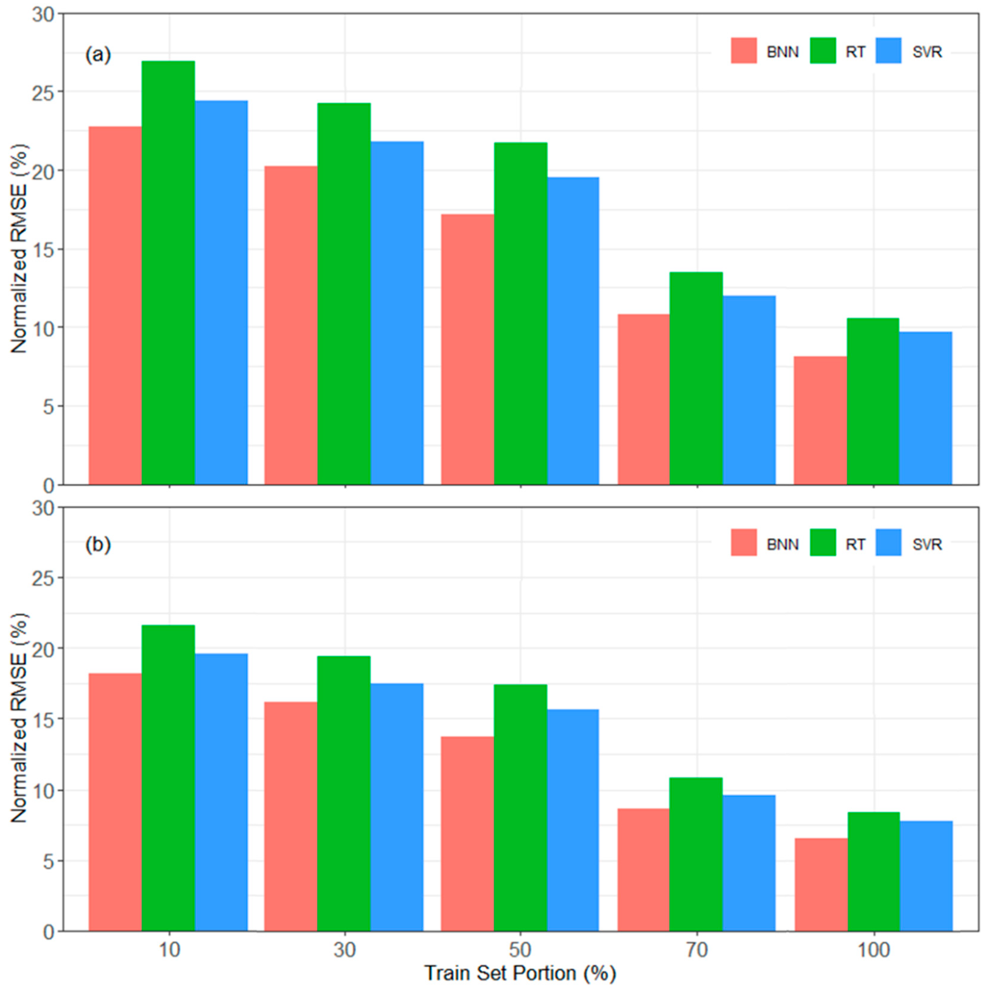
The influence of train set timeframe on the forecasting performance was examined by using different dataset portions (10%, 30%, 50%, and 70% of the first-year evaluation dataset) to train the machine learning models. In addition, the train set data portions comprised of both sequentially acquired and randomly sampled data from the entire first-year train set. The forecasting accuracy results obtained over the second-year evaluation period, presented in Figure 3, demonstrated that increasing the train set duration improves the forecasting performance of all investigated techniques. Figure 3a shows that the BNN provided the highest results when compared to the other models for all sequential training portions with a nRMSE of 19.14%, 17.33, 14.57%, 8.97%, and 6.51% when trained at 10%, 30%, 50%, 70%, and 100% portions of the train set, respectively. In addition, training with randomly sampled data yielded higher accuracies for all models compared to training sequentially. More specifically, the forecasting accuracy results when training all the models with train set portions comprising of random samples, depicted in Figure 3b, showed higher accuracies compared to the sequential data training regime. The obtained results demonstrated that for limited timeframe train sets, it is preferable to construct the data-driven models using random data samples from the entire training population over training sequentially.

3.3. Impact of Irradiance Condition Filtering

The dependency of the forecasting accuracy on data filtering and specifically, filtering at low (<600 W/m2) and high (≥600 W/m2) irradiance conditions, was further examined. The investigated machine learning models were trained with the filtered train sets and their performance was once again evaluated over the second-year evaluation test set. The day-ahead forecasting accuracies provided in Table 5, demonstrated that the application of the irradiance condition filter further improved the forecasting accuracies of all models (absolute difference in the range of 1.06–1.97% nRMSE and 0.71–2.22% MAPE when compared to the results without the application of an irradiance condition filter). Furthermore, the application of the high irradiance condition filter resulted in higher accuracies for all models. Specifically, the application of the high irradiance filter enhanced the performance of the BNN model that resulted in forecasting errors lower than 5% given by the nRMSE and MAPE. This renders the application of irradiance filtering necessary when training data-driven PV production forecasting models.

3.4. Optimized Day-Ahead PV Generation Forecasting Performance

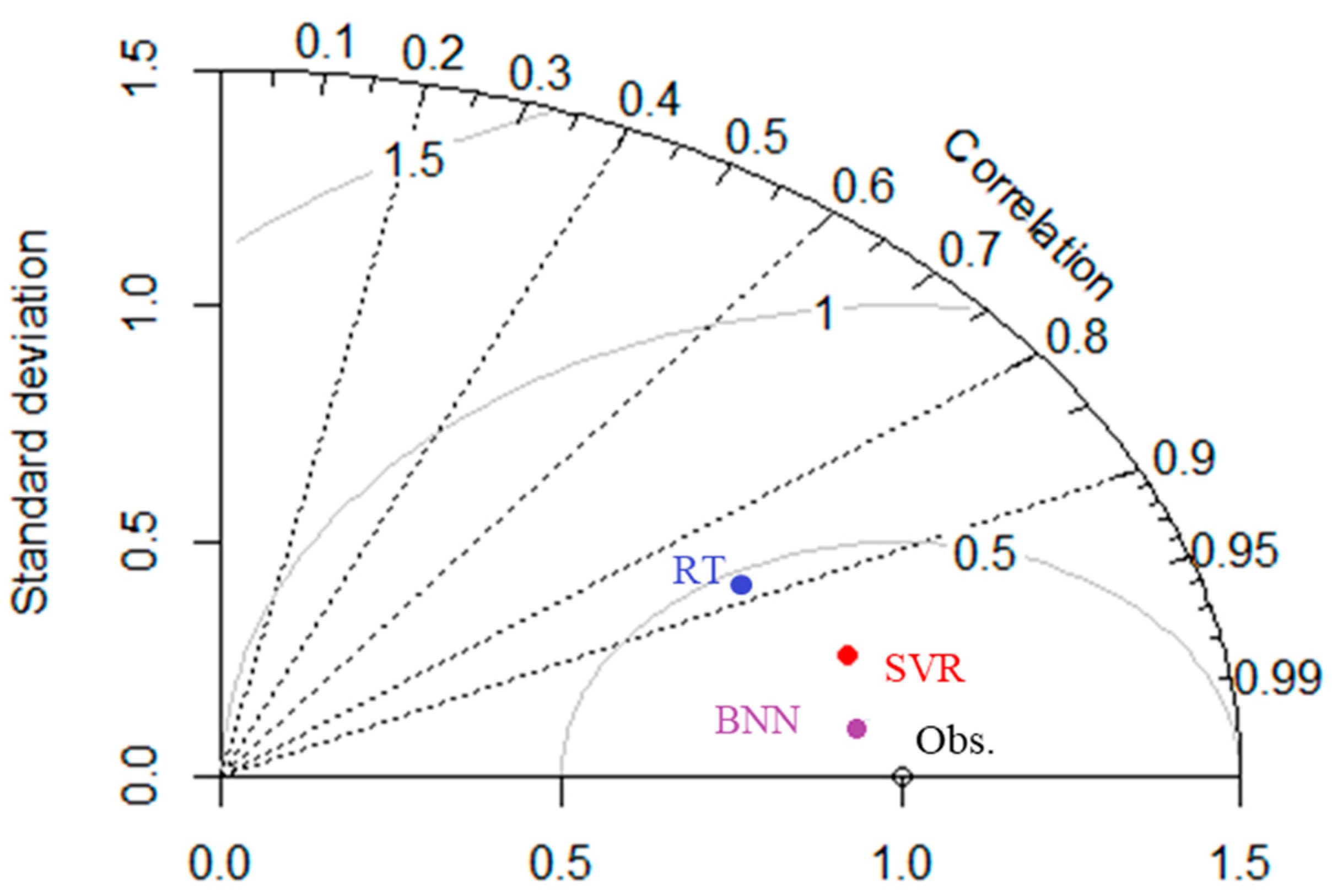
The training regime evaluation of the investigated machine learning models provided evidence that optimal performance is achieved when training using computed historical data inputs ( G H I _ F , T amb _ F , φ s and α ), employing the entire first-year dataset and filtering out data that are at low and moderate irradiance conditions (i.e., <600 W/m2). Initially, the Taylor diagram was used to benchmark the performance accuracy of the optimized models by comparing the heuristic distance between each model and the corresponding observations [61]. Specifically, the standard deviation and correlation of each model and actual data, presented in Figure 4, indicates that the best-performing model (the one with the lowest distance away from the actual observations) was the optimally trained BNN.
Figure 5 shows the daily PV power production forecasting accuracy (daily nRMSE) of the optimally trained models over the test set evaluation period, categorized according to the daily clearness index, k d . Overall, all models yielded daily nRMSE forecasts lower than 10% providing evidence that high performing forecasting models trained without employing on-site measurements, apart from the output power, can be constructed by applying the proposed methodology. As depicted in Figure 5a, the daily nRMSE results showed that the optimally designed BNN outperformed all other models exhibiting nRMSE lower than 5% (nRMSE = 4.53%), while the SVR and RT models provided in general less accurate results. Specifically, the nRMSE of the SVR and RT models over the test set period was 6.37% and 7.37%, presented in Figure 5b,c, respectively. Another important observation was that for most clear-sky days all the machine learning models exhibited nRMSE accuracies below 6%.
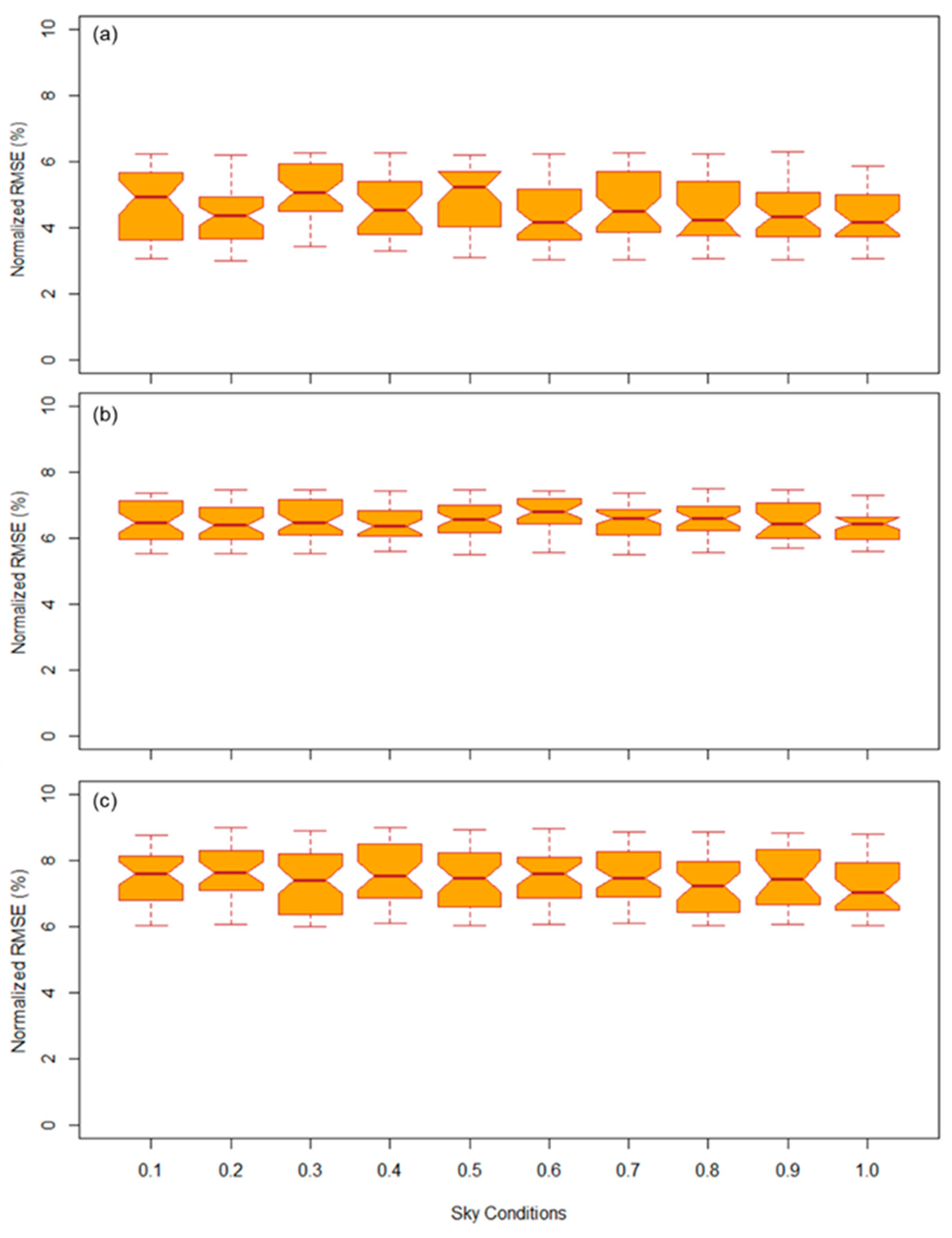
To gain insight into the performance of each model at different sky conditions a boxplot of the exhibited daily nRMSE at different k d bins over the test set evaluation period, was created. As depicted in Figure 6, all models exhibited similar daily nRMSE variations at all k d bins demonstrating that there are no underlying biases due to irradiance conditions. Qualitatively, it is evident that the BNN model yielded substantially more accurate results compared to the SVR and RT models for all k d bins, depicted in Figure 6a. To this end, an important outcome of this analysis was that the BNN consistently yielded robust results for the Cyprus’ climate, as it always provided accurate forecasts under any weather condition. Conversely, the SVR model exhibited the lowest residual dispersion as shown in Figure 6b. Consequently, the results indicate that the performance accuracy of the forecasting models is consistent at all sky conditions since the nRMSE values exhibit similar magnitude and variability.
More detailed information regarding the performance comparison of the investigated machine learning models, together with other evaluation metrics, is shown in Table 6. Specifically, Table 6 summarizes the performance of the resulting forecasting models over the test set evaluation period, based on commonly applied forecasting performance metrics (nRMSE, RMSE, MAPE, MBE, and SS). In this framework, the results in Table 6 confirm that the optimally devised BNN consistently outperformed the other machine learning models (SVR and RT). The forecasting capabilities of the SVR and RT models can be considered as equivalent in this case, since the exhibited nRMSE absolute difference of these models was 1%. Moreover, the results indicated that the application of machine learning achieved higher relative improvement over the reference PM since the SS ranged from 53.71% to 78.33%. To further assess the direction of the forecasted bias, the obtained nMBE of all models showed that power generation was underestimated (between 2.89–5.42%).
A residual analysis was conducted to further assess the quality of the models and the statistical significance of the nRMSE difference. The residuals (the difference between the actual and forecasted values) of the test set period were examined for normality using the Shapiro–Wilk normality test [62]. The statistic tests the null hypothesis that the residuals come from a normally distributed population. The performed normality test considering a significance level of 5% provided evidence that the null hypothesis is rejected and that there is evidence that the data tested are not normally distributed since the p value obtained for each model was less than 0.05 (BNN = 0.014, SVR = 0.027 and RT = 0.024), therefore, this indicates a statistically significant test result (P ≤ 0.05) meaning that the test hypothesis is false or should be rejected, indicating that the residuals of the forecasting models had been affected from the observed data.
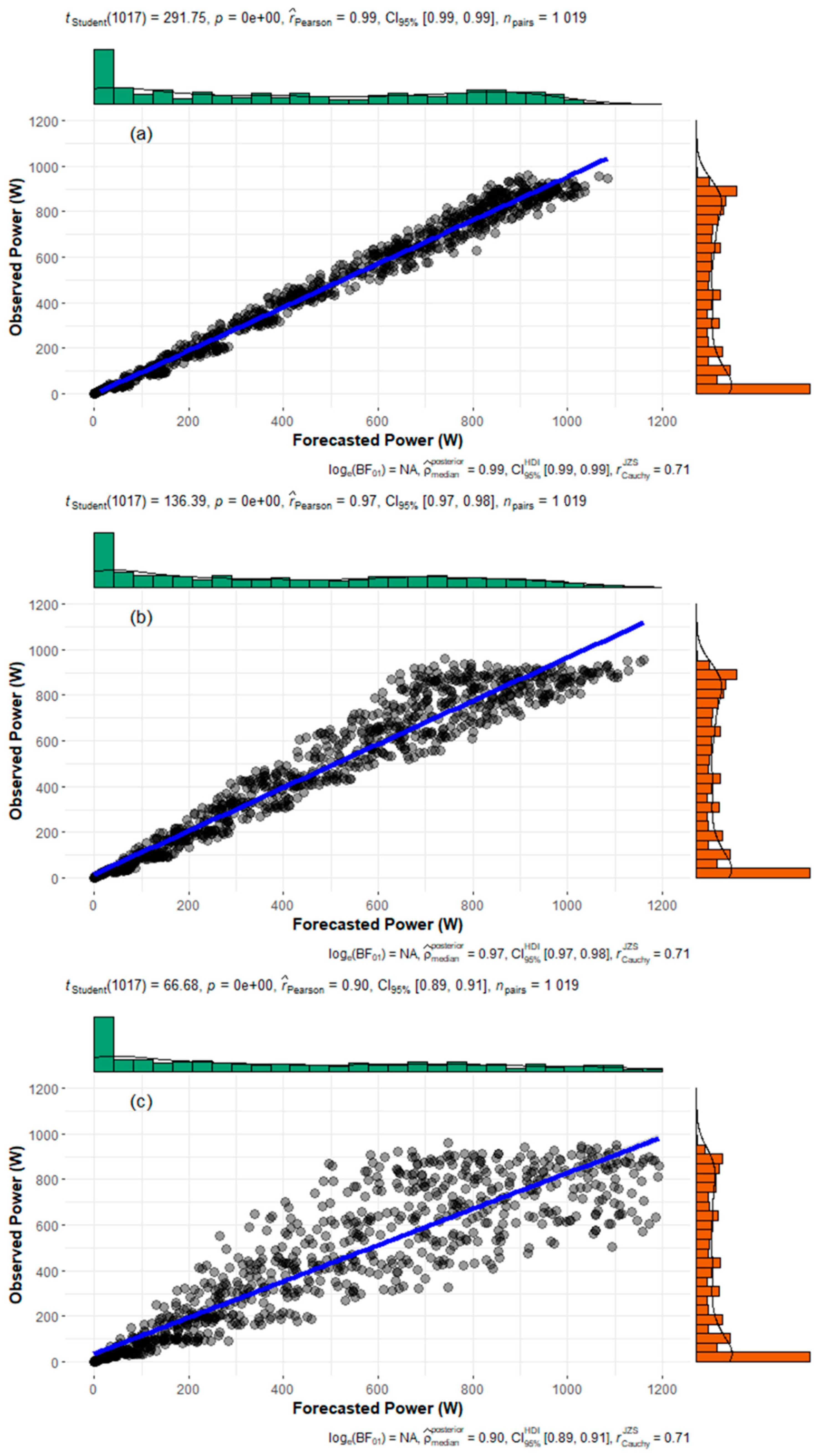
Furthermore, Figure 7 exhibits the scatterplots of the observed against the forecasted power obtained from all the investigated forecasting models. The comparison shows that the variability was exhibited by the forecasts of the BNN model with Pearson correlation (r) of r = 0.99, as depicted in Figure 7a. Slightly higher variability was exhibited by the SVR model with r = 0.97, shown in Figure 7b, while the highest scattering was obtained by the RT forecasts r = 0.90, depicted in Figure 7c. Additionally, the BNN model residuals are concentrated around the blue fitting line, indicating clos fit at all power levels. Conversely, the residuals of both the SVR and RT models present higher variability at high irradiance conditions where PV output is maximized.
Finally, the statistical significance of the nRMSE difference of all investigated models was evaluated by using the Wilcoxon signed-rank test [63], considering a significance level of 5%. The test was used to assess the statistical significance of the nRMSE differences between the models, by using all the hourly errors to investigate whether the observed difference in model skill is likely due to a difference of the models or statistical chance. As a result, after comparing every possible residual pair of the forecasting algorithms, the obtained results provided evidence that the differences between the investigated models are statistically significant (the differences are due to the models and not by chance) since the highest p value was obtained when comparing the BNN and SVR (p value equal to 0.037), indicating that the BNN model has a confidence interval of 96.3% over the SVR model.

4. Discussion

In this work, a comparative day-ahead forecasting performance analysis of different machine learning models was presented. Within this framework, the performed data-driven training regime analysis revealed useful information for the implementation of an accurate day-ahead PV production forecasting methodology with minimal input measured features. In summary, the following findings were obtained throughout the commenced analysis:
  • Accurate day-ahead PV production forecasts were achieved without utilizing onsite weather measurements by inputting data that were computed from NWP models and solar position algorithms ( G H I _ F , T amb _ F , φ s and α ) to machine learning models. The application of calculated input data compared to training with the respective on-site measured data provided maximum absolute improvements of up to 0.77% and 1.31% for the nRMSE and MAPE, respectively. This improvement is attributed to the correction of underlying biases of NWP forecasted data.
  • Training the machine learning models at larger timeframes resulted in lower errors. This is attributed to the generic functionality of data-driven algorithms of capturing hidden behaviors from larger amounts of data.
  • The application of irradiance filtering when training data-driven PV production forecasting models enhanced the performance of the constructed models. Specifically, the forecasting accuracy of all models was improved from the application of the irradiance condition filter (absolute difference in the range of 1.06–1.97% nRMSE and 0.71–2.22% MAPE when compared to the results without the application of an irradiance condition filter). The application of the high irradiance condition filter resulted in lower errors for all models rendering this filtering stage an important step in day-ahead data-driven methodologies. This can be attributed to the fact that low and medium irradiance conditions (<0.6 kW/m2) are associated with a higher power output dispersion (low-light and thermal effects), which in turn decreases the forecasting accuracy.
  • Overall, the adoption of BNN principles outperformed all other investigated models (SVR and RT). More specifically, the study showed that the optimally trained BNN consistently outperformed all other models exhibiting nRMSE lower than 5% (nRMSE = 4.53%), while the SVR and RT models provided in general less accurate results. Several reasons to explain this effect include the ability of BNNs to simulate multiple possible models with an associated probability distribution and to become more certain with increasing data shares. The BNN model was substantially more accurate compared to the SVR and RT models for all sky conditions. This renders BNN approaches applicable for forecasting studies and favorable over other elaborate and computer intensive techniques.
Furthermore, since the main objective of this study was to implement a unified methodology with minimal input features, the obtained results demonstrated that accurate day-ahead PV production forecasting machine learning models can be constructed by entirely inputting computed parameters and applying a high irradiance condition filter to a 1-year train set. It is important to mention that the results of the specific work were location- and system-specific, therefore by applying datasets from other systems and/or locations, the respective results might indicate variations.
The proposed generalized methodology can be applied to larger PV plants with identical results. This can be achieved by employing an intermediate PV power normalization step (normalize all power measurements to the rated capacity of the PV system) before commencing the training, which will enable forecasting of the PV power production irrespective to the capacity of the plant. At the output stage, the normalized power forecasts can be scaled up to the rated power of the investigated system. Optionally, the proposed method can operate on either the output data recorded from a monitoring system, smart meter at the point of interconnection (POI) and at the output of a central inverter. In this case no normalization is required since the model is directly trained using the power output of the entire plant.
Finally, this work focuses on the application of day-ahead PV production forecasting as an enabling cost-effective technology that will improve the flexibility and observability of the grid. According to the European Technology Innovation Platform for PV (ETIP PV) accurate day-ahead PV production forecasting is a necessity for utility operators for determining operation reserve requirements, for distribution system operators (DSOs) and microgrid operators for the optimal day-ahead flexible commitment of resources and PV plant operators for energy trading and management of storage systems [64]. As an example, a utility scale 10 MWp PV power plant located in regions with high irradiance (annual irradiation of 2000 kWh/m2) and participating in the wholesale market, produces 17,000 MWh/year (assuming a PR of 85%). An absolute forecasting improvement of 2% provides approximately 11,050 MWh/year of excess energy that is not curtailed due to forecasting errors. Moreover, this excess energy can be traded in the Energy market providing additional revenue of approximately €8M (at an Energy trading cost of 70 €/MWh).

5. Conclusions

Photovoltaic (PV) power production forecasting is an efficient cost-effective tool for grid management and a critical decisive function for system reliability at high PV shares. This paper presented a comparative analysis towards implementing a unified methodology for accurately forecasting the day-ahead production of PV power plants with minimal measured data. To this end, the method included the data acquisition, construction, and optimization of PV predictive models based on machine learning (Bayesian neural network (BNN), support vector regression (SVR) and regression tree (RT)) using different supervised learning regimes whereas their performance was verified using consistent metrics. The benchmarking was carried out using two-year field data from a test-bench PV system installed in Nicosia, Cyprus, enabling homogenous conditions for such evaluations.
The supervised learning analysis showed that high-performing models can be constructed by entirely utilizing data that were computed from numerical weather predictions (NWP) models and solar position algorithms. This is an important outcome since accurate forecasting models can be constructed in the absence of on-site weather measurements.
Additionally, the amount of training dataset timeframe was directly influencing the accuracy of the forecasts since increasing the train set duration improved the forecasting performance of all investigated techniques. For low resolution datasets the application of training all the models with train set portions comprising of random samples showed higher accuracies compared to the sequential data training regime.
Moreover, the application of an irradiance filter further improved the forecasting accuracies of all models. Specifically, the high irradiance filter further enhanced the performance of the BNN model that resulted to forecasting errors lower than 5%, demonstrating that the predictive accuracy of the models was enhanced by data filtering.
Finally, the comparative analysis of the optimally devised machine learning models showed that all the models achieved relative improvements over the reference model (SS results ranged from 53.71% to 78.33%). The performance accuracy of the forecasting models was stable at all sky conditions since the obtained normalized root mean square error (nRMSE) values exhibited similar magnitudes and variabilities. The optimally trained BNN outperformed all other models (SVR and RT) and consistently achieved the lowest forecasting errors (nRMSE = 4.53% and mean absolute percentage error (MAPE) = 3.17%), over the test set evaluation period. The ability of the BNN model to adapt to frequent fluctuations and its relatively low complexity and optimization with respect to the computational efficiency further highlight its overall performance.

Author Contributions

Conceptualization, S.T.; data curation, S.T. and M.K.; formal analysis, S.T. methodology, S.T. and G.M.; investigation, G.M., S.T. and C.S.; project administration, G.M. and G.E.G.; resources, G.E.G. and G.M.; software, S.T.; validation, M.T., S.T. and C.S.; visualization, S.T., M.T. and M.K.; writing—original draft, S.T.; writing—review and editing M.T., G.M., C.S. and G.E.G. All authors have read and agreed to the published version of the manuscript.

Funding

This work was funded through the ELECTRA project, which is co-financed by the European Regional Development Fund of the European Union under the grant agreement number INTEGRATED/0918/0071. The authors from the University of Cyprus would also like to acknowledge the financial support from the Research & Innovation Foundation of Cyprus.

Institutional Review Board Statement

Not applicable.

Informed Consent Statement

Not applicable.

Data Availability Statement

The data presented in this study are available on request from the corresponding author. The data are not publicly available due to privacy reasons.

Acknowledgments

Sandia National Laboratories is a multimission laboratory managed and operated by the National Technology & Engineering Solutions of Sandia, LLC, a wholly owned subsidiary of Honeywell International Inc., for the U.S. Department of Energy’s National Nuclear Security Administration under contract DE-NA0003525. This paper describes objective technical results and analysis. Any subjective views or opinions that might be expressed in the paper do not necessarily represent the views of the U.S. Department of Energy or the United States Government.

Conflicts of Interest

The authors declare no conflict of interest.

References

  1. International Energy Agency. Electricity Security in Tomorrow’s Power Systems. 2020. Available online: https://www.iea.org/articles/electricity-security-in-tomorrow-s-power-systems (accessed on 17 December 2020).
  2. International Energy Agency. Renewables 2019: Market Analysis and Forecast from 2019 to 2024. 2019. Available online: https://www.iea.org/reports/renewables-2019 (accessed on 10 December 2020).
  3. International Energy Agency. Introduction to System Integration of Renewables: Decarbonising while Meeting Growing Demand. 2020. Available online: https://www.iea.org/reports/introduction-to-system-integration-of-renewables (accessed on 15 November 2020).
  4. Sadeghian, H.; Wang, Z. A novel impact-assessment framework for distributed PV installations in low-voltage secondary networks. Renew. Energy 2020, 147, 2179–2194. [Google Scholar] [CrossRef]
  5. Mahoor, M.; Majzoobi, A.; Khodaei, A. Distribution asset management through coordinated microgrid scheduling. IET Smart Grid 2018, 1, 159–168. [Google Scholar] [CrossRef]
  6. International Renewable Energy Agency. Innovation Landscape for a Renewable-Powered Future. 2019. Available online: https://www.irena.org/publications/2019/Feb/Innovation-landscape-for-a-renewable-powered-future (accessed on 10 November 2020).
  7. Inman, R.H.; Pedro, H.T.C.; Coimbra, C.F.M. Solar forecasting methods for renewable energy integration. Prog. Energy Combust. Sci. 2013, 39, 535–576. [Google Scholar] [CrossRef]
  8. Das, U.K.; Tey, K.S.; Seyedmahmoudian, M.; Mekhilef, S.; Idris, M.Y.I.; Van Deventer, W.; Horanc, B.; Stojcevskid, A. Forecasting of photovoltaic power generation and model optimization: A review. Renew. Sustain. Energy Rev. 2018, 81, 912–928. [Google Scholar] [CrossRef]
  9. International Energy Agency. Photovoltaic and Solar Forecasting: State of Art. 2013. Available online: https://iea-pvps.org/key-topics/photovoltaics-and-solar-forecasting-state-of-art-report-t1401-2013/ (accessed on 5 December 2020).
  10. Alanzi, M.; Alanzi, A.; Khodaei, A. Long-Term Solar Generation Forecasting. In Proceedings of the IEEE/PES Transmission and Distribution Conference and Exposition (T&D), Dallas, TX, USA, 3–5 May 2016; pp. 1–5. [Google Scholar]
  11. National Centers for Environmental Information. Global Forecast System. 2020. Available online: https://www.ncdc.noaa.gov/data-access/model-data/model-datasets/global-forcast-system-gfs (accessed on 17 November 2020).
  12. Perez, R.; Lorenz, E.; Pelland, S.; Beauharnois, M.; Van Knowe, G.; Hemker, K.J.; Heinemann, D.; Remund, J.; Mller, S.; Traunmller, W.; et al. Comparison of numerical weather prediction solar irradiance forecasts in the US, Canada and Europe. Sol. Energy 2013, 94, 305–326. [Google Scholar] [CrossRef]
  13. Voyant, C.; Muselli, M.; Paoli, C.; Nivet, M. Numerical weather prediction (NWP) and hybrid ARMA/ANN model to predict global radiation. Energy 2012, 39, 341–355. [Google Scholar] [CrossRef] [Green Version]
  14. Lara-Fanego, V.; Ruiz-Arias, J.; Pozo-Vazquez, D.; Santos-Alamillos, F.; Tovar-Pescador, J. Evaluation of the WRF model solar irradiance forecasts in Andalusia (southern Spain). Sol. Energy 2012, 86, 2200–2217. [Google Scholar] [CrossRef]
  15. Mathiesen, P.; Collier, C.; Kleissl, J. A high-resolution, cloud-assimilating numerical weather prediction model for solar irradiance forecasting. Sol. Energy 2013, 92, 47–61. [Google Scholar]
  16. Pelland, S.; Galanis, G.; Kallos, G. Solar and photovoltaic forecasting through post-processing of the global environmental multiscale numerical weather prediction model. Prog. Photovolt. Res. Appl. 2013, 21, 284–296. [Google Scholar] [CrossRef]
  17. Ohtake, H.; Shimose, K.; Fonseca, J.; Takashima, T.; Oozeki, T.; Yamada, Y. Accuracy of the solar irradiance forecasts of the Japan Meteorological Agency mesoscale model for the Kanto region, Japan. Sol. Energy 2013, 98, 138–152. [Google Scholar] [CrossRef]
  18. National Center for Atmospheric Research. Weather Research and Forecasting Model. 2020. Available online: https://www.mmm.ucar.edu/weather-research-and-forecasting-model (accessed on 17 December 2020).
  19. Jimenez, P.A.; Hacker, J.P.; Dudhia, J.; Haupt, S.E.; Ruiz-Arias, J.A.; Gueymard, C.A.; Thompson, G.; Eidhammer, T.; Deng, A. WRF-Solar: Description and clear-sky assessment of an augmented NWP model for solar power prediction. Bull. Am. Meteorol. Soc. 2016, 97, 1249–1264. [Google Scholar] [CrossRef]
  20. Da Silva Fonseca, J.G.; Oozeki, T.; Ohtake, H.; Shimose, K.I.; Takashima, T.; Ogimoto, K. Forecasting regional photovoltaic power generation—A comparison of strategies to obtain one-day-ahead data. Energy Procedia 2014, 57, 1337–1345. [Google Scholar]
  21. Ashraf, I.; Chandra, A. Artificial neural network based models for forecasting electricity generation of grid connected solar PV power plant. Int. J. Glob. Energy Issues 2004, 21, 119–130. [Google Scholar] [CrossRef]
  22. Caputo, D.; Grimaccia, F.; Mussetta, M.; Zich, R.E. Photovoltaic plants predictive model by means of ANN trained by a hybrid evolutionary algorithm. In Proceedings of the 2010 International Joint Conference on Neural Networks (IJCNN), Barcelona, Spain, 18–23 July 2010; pp. 1–6. [Google Scholar]
  23. Kalogirou, S.A. Applications of artificial neural-networks for energy systems. Appl. Energy 2000, 67, 17–35. [Google Scholar] [CrossRef]
  24. Mellit, A.; Pavan, A.M. A 24-h forecast of solar irradiance using artificial neural network: Application for performance prediction of a grid-connected PV plant at Trieste, Italy. Sol. Energy 2010, 84, 807–821. [Google Scholar] [CrossRef]
  25. Almonacid, F.; Pérez-Higueras, P.J.; Fernández, E.F.; Hontoria, L. A methodology based on dynamic artificial neural network for short-term forecasting of the power output of a PV generator. Energy Convers. Manag. 2014, 85, 389–398. [Google Scholar] [CrossRef]
  26. Yona, A.; Senjyu, T.; Saber, A.Y.; Funabashi, T.; Sekine, H.; Kim, C.H. Application of neural network to 24-hour-ahead generating power forecasting for PV system. In Proceedings of the 2007 International Conference on Intelligent Systems Applications to Power Systems, Nigata, Japan, 5–8 November 2007; pp. 1–6. [Google Scholar]
  27. Zhang, Y.; Beaudin, M.; Taheri, R.; Zareipour, H.; Wood, D. Day-ahead power output forecasting for small-scale solar photovoltaic electricity generators. IEEE Trans. Smart Grid 2015, 6, 2253–2262. [Google Scholar] [CrossRef]
  28. Wang, S.; Zhang, N.; Zhao, Y.; Zhan, J. Photovoltaic system power forecasting based on combined grey model and BP neural network. In Proceedings of the 2011 International Conference on Electrical and Control Engineering, Yichang, China, 16–18 September 2011; pp. 1–6. [Google Scholar]
  29. Mellit, A.; Massi Pavan, A.; Lughi, V. Short-term forecasting of power production in a large-scale photovoltaic plant. Sol. Energy 2014, 105, 401–413. [Google Scholar] [CrossRef]
  30. Zamo, M.; Mestre, O.; Arbogast, P.; Pannekoucke, O. A benchmark of statistical regression methods for short-term forecasting of photovoltaic electricity production. Part I: Probabilistic forecast of daily production. Sol. Energy 2014, 105, 792–803. [Google Scholar] [CrossRef]
  31. Eseye, A.T.; Zhang, J.; Zheng, D. Short-term photovoltaic solar power forecasting using a hybrid Wavelet-PSO-SVM model based on SCADA and meteorological information. Renew. Energy 2018, 118, 357–367. [Google Scholar] [CrossRef]
  32. Preda, S.; Oprea, S.; Bâra, A.; Belciu, A. PV forecasting using support vector machine learning in a big data analytics context. Symmetry 2018, 10, 748. [Google Scholar] [CrossRef] [Green Version]
  33. Zendehboudia, A.; Baseerb, M.A.; Saidurcd, R. Application of support vector machine models for forecasting solar and wind energy resources: A review. J. Clean. Prod. 2018, 199, 272–285. [Google Scholar] [CrossRef]
  34. Zhu, H.; Lian, W.; Lu, L.; Dai, S.; Hu, Y. An improved forecasting method for photovoltaic power based on adaptive BP neural network with a scrolling time window. Energies 2017, 10, 1542. [Google Scholar] [CrossRef] [Green Version]
  35. Dumitru, C.; Gligor, A.; Enachescu, C. Solar photovoltaic energy production Forecast Using Neural Networks. Procedia Technol. 2016, 22, 808–815. [Google Scholar] [CrossRef] [Green Version]
  36. Liu, L.; Zhao, Y.; Chang, D.; Xie, J.; Ma, Z.; Sun, Q.; Yin, H.; Wennersten, R. Prediction of short-term PV power output and uncertainty analysis. Appl. Energy 2018, 228, 700–711. [Google Scholar] [CrossRef]
  37. Benali, L.; Notton, G.; Fouilloy, A.; Voyant, C.; Dizene, R. Solar radiation forecasting using artificial neural network and random forest methods: Application to normal beam, horizontal diffuse and global components. Renew. Energy 2019, 132, 871–884. [Google Scholar] [CrossRef]
  38. Prasad, R.; Ali, M.; Kwan, P.; Khan, H. Designing a multi-stage multivariate empirical mode decomposition coupled with ant colony optimization and random forest model to forecast monthly solar radiation. Appl. Energy 2019, 236, 778–792. [Google Scholar] [CrossRef]
  39. Torres, J.F.; Troncoso, A.; Koprinska, I.; Wang, Z.; Martínez-Álvarez, F. Big data solar power forecasting based on deep learning and multiple data sources. Expert Syst. 2019, 39, 1–14. [Google Scholar] [CrossRef]
  40. Wang, K.; Qi, X.; Liu, H. A comparison of day-ahead photovoltaic power forecasting models based on deep learning neural network. Appl. Energy 2019, 251, 1–14. [Google Scholar] [CrossRef]
  41. Abdel-Nasser, M.; Mahmoud, K. Accurate photovoltaic power forecasting models using deep LSTM-RNN. Neural Comput. Appl. 2017, 31, 2727–2740. [Google Scholar] [CrossRef]
  42. Wang, H.; Yi, H.; Peng, J.; Wang, G.; Liu, Y.; Jiang, H.; Liu, W. Deterministic and probabilistic forecasting of photovoltaic power based on deep convolutional neural network. Energy Convers. Manag. 2017, 153, 409–422. [Google Scholar] [CrossRef]
  43. Theocharides, S.; Makrides, G.; Georghiou, G.E.; Kyprianou, A. Machine learning algorithms for photovoltaic system power output prediction. In Proceedings of the 2018 IEEE International Energy Conference, Limassol, Cyprus, 3–7 June 2018; pp. 1–6. [Google Scholar]
  44. Glassley, W.; Kleissl, J.; Dam, C.P.; Shiu, H.; Huang, J. California Renewable Energy Forecasting, Resource Data and Mapping Executive Summary; Public Interest Energy Research (PIER) Program; California Energy Commission: Sacramento, CA, USA, 2010; pp. 1–135.
  45. Bermejo, J.H.; Fernández, J.F.; Polo, F.O.; Márquez, A.C. A review of the use of artificial neural network models for energy and reliability prediction. A study of the solar PV, hydraulic and wind energy sources. Appl. Sci. 2019, 9, 1844. [Google Scholar] [CrossRef] [Green Version]
  46. Raza, M.Q.; Nadarajah, M.; Ekanayake, C. On recent advances in PV output power forecast. Sol. Energy 2016, 136, 125–144. [Google Scholar] [CrossRef]
  47. Nespoli, A.; Ogliari, E.; Leva, S.; Massi Pavan, A.; Mellit, A.; Lughi, V.; Dolara, A. Day-Ahead Photovoltaic Forecasting: A Comparison of the Most Effective Techniques. Energies 2019, 12, 1621. [Google Scholar] [CrossRef] [Green Version]
  48. Chen, C.; Duan, S.; Cai, T.; Liu, B. Online 24-h solar power forecasting based on weather type classification using artificial neural network. Sol. Energy 2011, 85, 2856–2870. [Google Scholar] [CrossRef]
  49. Dolara, A.; Grimaccia, F.; Leva, S.; Mussetta, M.; Ogliari, E. A physical hybrid artificial neural network for short term forecasting of PV plant power output. Energies 2015, 8, 1138–1153. [Google Scholar] [CrossRef] [Green Version]
  50. IEC 61724-1. Photovoltaic System Performance—Part 1: Monitoring; IEC: Geneva, Switzerland, 2017. [Google Scholar]
  51. Reda, I.; Adreas, A. Solar position algorithm for solar radiation applications. Sol. Energy 2004, 76, 577–589. [Google Scholar] [CrossRef]
  52. R Core Team. R: A Language and Environment for Statistical Computing; R Foundation for Statistical Computing: Vienna, Austria, 2019. [Google Scholar]
  53. Livera, A.; Theristis, M.; Koumpli, E.; Theocharides, S.; Makrides, G.; Joshua, S.S.; Georghiou, G.E. Data processing and quality verification for improved photovoltaic performance and reliability analytics. Prog. Photovoltaics Res. Appl. 2020. [Google Scholar] [CrossRef]
  54. Theocharides, S.; Makrides, G.; Livera, A.; Theristis, M.; Kaimakis, P.; Georghiou, G.E. Day-ahead photovoltaic power production forecasting methodology based on machine learning and statistical post-processing. Appl. Energy 2020, 268, 1–14. [Google Scholar] [CrossRef]
  55. Jospin, L.; Buntine, W.; Boussaid, F.; Laga, H.; Bennamoun, M. Hands-on Bayesian neural networks—A tutorial for deep learning users. ACM Comput. Surv. 2020, 1, 1–35. [Google Scholar]
  56. Polson, N.; Sokolov, V. Deep learning: A Bayesian perspective. Bayesian Anal. 2017, 12, 1275–1304. [Google Scholar] [CrossRef]
  57. Zhou, Z. Ensemble Methods: Foundations and Algorithms, 1st ed.; Chapman and Hall/CRC: Boca Raton, FL, USA, 2012; pp. 1–236. [Google Scholar]
  58. MacKay, D.J.C. Bayesian Interpolation. Neural Comput. 1992, 4, 415–447. [Google Scholar] [CrossRef]
  59. Smola, A.J.; Schölkopf, B. A tutorial on support vector regression. Stat. Comput. 2004, 14, 199–222. [Google Scholar] [CrossRef] [Green Version]
  60. Gordon, A.D.; Breiman, L.; Friedman, J.H.; Olshen, R.A.; Stone, C.J. Classification and Regression Trees. Biometrics 1984, 40, 358–361. [Google Scholar] [CrossRef] [Green Version]
  61. Taylor, K.E. Summarizing multiple aspects of model performance in a single diagram. J. Geophys. Res. 2001, 106, 7183–7192. [Google Scholar] [CrossRef]
  62. Shapiro, S.S.; Wilk, M.B. An analysis of variance test for normality (complete samples). Biometrika 1965, 52, 591–611. [Google Scholar] [CrossRef]
  63. Wilcoxon, F. Individual comparisons by ranking methods. Biom. Bull. 1945, 1, 80–83. [Google Scholar] [CrossRef]
  64. European Technology and Innovation Platform. Accessing the Need for Better Forecasting and Observability of PV; ETIP PV—SEC II; European Union: Brussels, Belgium, 2017; pp. 1–21. [Google Scholar]
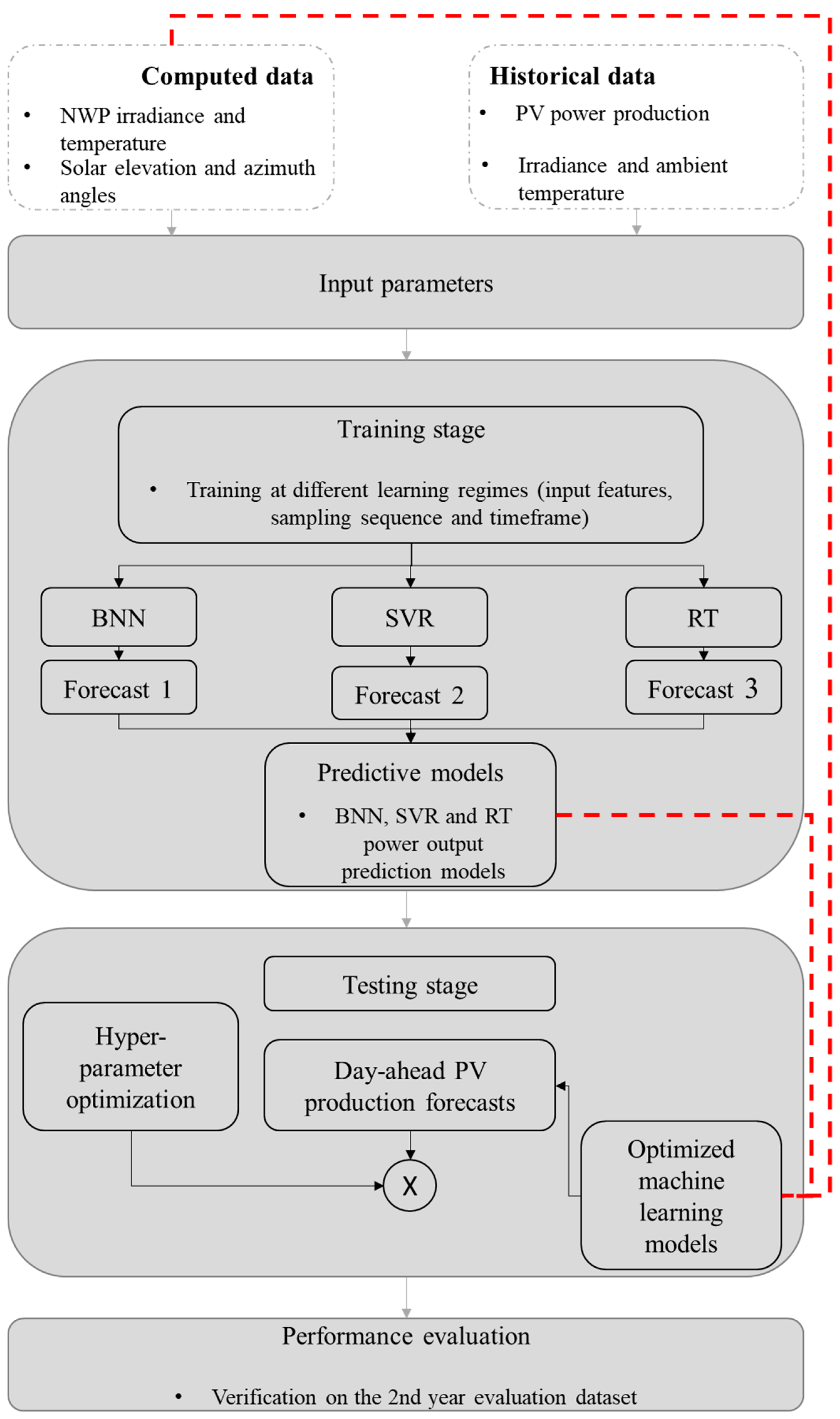
Figure 1. Flowchart of the proposed day-ahead photovoltaic (PV) production forecasting methodology.
Energies 14 01081 g001
Figure 2. Test-bench PV system comprising of a polycrystalline silicon (poly-c Si) photovoltaic (PV)string, sensor network and data acquisition (DAQ) monitoring system, at the FOSS Research Centre in Nicosia, Cyprus.
Energies 14 01081 g002
Figure 3. Test set nRMSE of the machine learning models at different train sets (10%, 30%, 50%, 70%, and 100% of the entire dataset) trained with: (a) Sequential measurements; (b) randomly sampled measurements.
Energies 14 01081 g003
Figure 4. Taylor diagram of the forecasted Bayesian neural network (BNN) (purple dot), support vector regression (SVR) (red dot), and regression tree (RT) (blue dot) against the observed power values (white dot), over the test set evaluation period.
Energies 14 01081 g004
Figure 5. Day-ahead photovoltaic (PV) power production forecasting accuracy given by the daily nRMSE when applying over the test set evaluation period the optimally trained machine learning models of: (a) Bayesian neural network (BNN); (b) support vector regression (SVR); (c) regression tree (RT).The red dashed line indicates the average nRMSE over the test set evaluation period.
Energies 14 01081 g005
Figure 6. Boxplot of daily nRMSE accuracy at different sky conditions over the test set evaluation period for the optimally trained machine learning models of: (a) Bayesian neural network (BNN); (b) support vector regression (SVR); (c) regression tree (RT). The red line indicates the median value.
Energies 14 01081 g006
Figure 7. Scatter plots of the observed against forecasted power for the: (a) Bayesian neural network (BNN); (b) support vector regression (SVR); (c) regression tree (RT). The blue line demonstrates the linear fit.
Energies 14 01081 g007
Table 1. Technical information of data acquisition (DAQ) system and sensor network.
ParameterManufacturer ModelManufacturer’s HeadquartersAccuracy
Data acquisitionCampbell Scientific CR1000Logan, UT, USA±0.06%
Ambient temperatureRotronic HC2A-S3Bassersdorf, Switzerland ±0.1 °C at 23 °C
In-plane irradianceKipp Zonen CMP11Delft, The Netherlands±2% expected daily accuracy, ±20 W/m2 for 1000 W/m2
DC voltageMuller Ziegler UgtGunzenhausen Germany±0.5%
DC currentMuller Ziegler IgtGunzenhausen Germany±0.5%
AC energyMuller Ziegler EZWGunzenhausen Germany±1%
Table 2. Train set features, data timeframe partition, and sampling regime.
InputsTimeframe PartitionSamplingOutput
G I , T amb , φ s and α 10–70% (at 20% resolution)Sequential/Random P mp
G I , T amb , φ s and α 100% (entire year)- P mp
G H I _ F , T amb _ F , φ s and α 10–70% (at 20% resolution)Sequential/Random P mp
G H I _ F , T amb _ F , φ s and α 100% (entire year)- P mp
Table 3. Day-ahead photovoltaic (PV) production forecasting accuracy comparison of different machine learning predictive models trained using measured historical data, over the test set evaluation period.
ModelnRMSE (%)MAPE (%)
BNN6.956.07
SVR8.517.92
RT8.978.12
Table 4. Day-ahead photovoltaic (PV) production forecasting accuracy comparison of the machine learning predictive models trained using computed historical data, over the test set evaluation period.
ModelnRMSE (%)MAPE (%)
BNN6.515.39
SVR7.746.61
RT8.436.98
Table 5. Day-ahead photovoltaic (PV) production forecasting accuracy comparison of the machine learning predictive models trained at different irradiance condition levels, over the test set evaluation period.
BNNSVRRT
IrradiancenRMSE (%)MAPE (%)nRMSE (%)MAPE (%)nRMSE (%)MAPE (%)
<600 W/m25.323.786.826.148.097.85
≥600 W/m24.533.176.375.837.376.27
No Filter6.515.397.746.618.436.98
Table 6. Performance accuracy (mean absolute percentage error (MAPE), root mean square error (RMSE), normalized RMSE (nRMSE), normalized mean biased error (nMBE), and skill score (SS)) of the different data-driven models over the test set evaluation period.
Performance Metrics
ModelsMAPE (%)RMSE (W)nRMSE (%)nMBE (%)SS (%)
BNN3.1753.224.532.8978.33
SVR5.8381.896.374.2663.14
RT6.2786.597.375.4253.71
Publisher’s Note: MDPI stays neutral with regard to jurisdictional claims in published maps and institutional affiliations.