
Photovoltaic Power Forecasting: Assessment of the Impact of Multiple Sources of Spatio-Temporal Data on Forecast Accuracy


Abstract
1. Introduction
2. Experimental Framework for Spatio-Temporal Forecasting
2.1. PV Power Data and Weather Forecasts
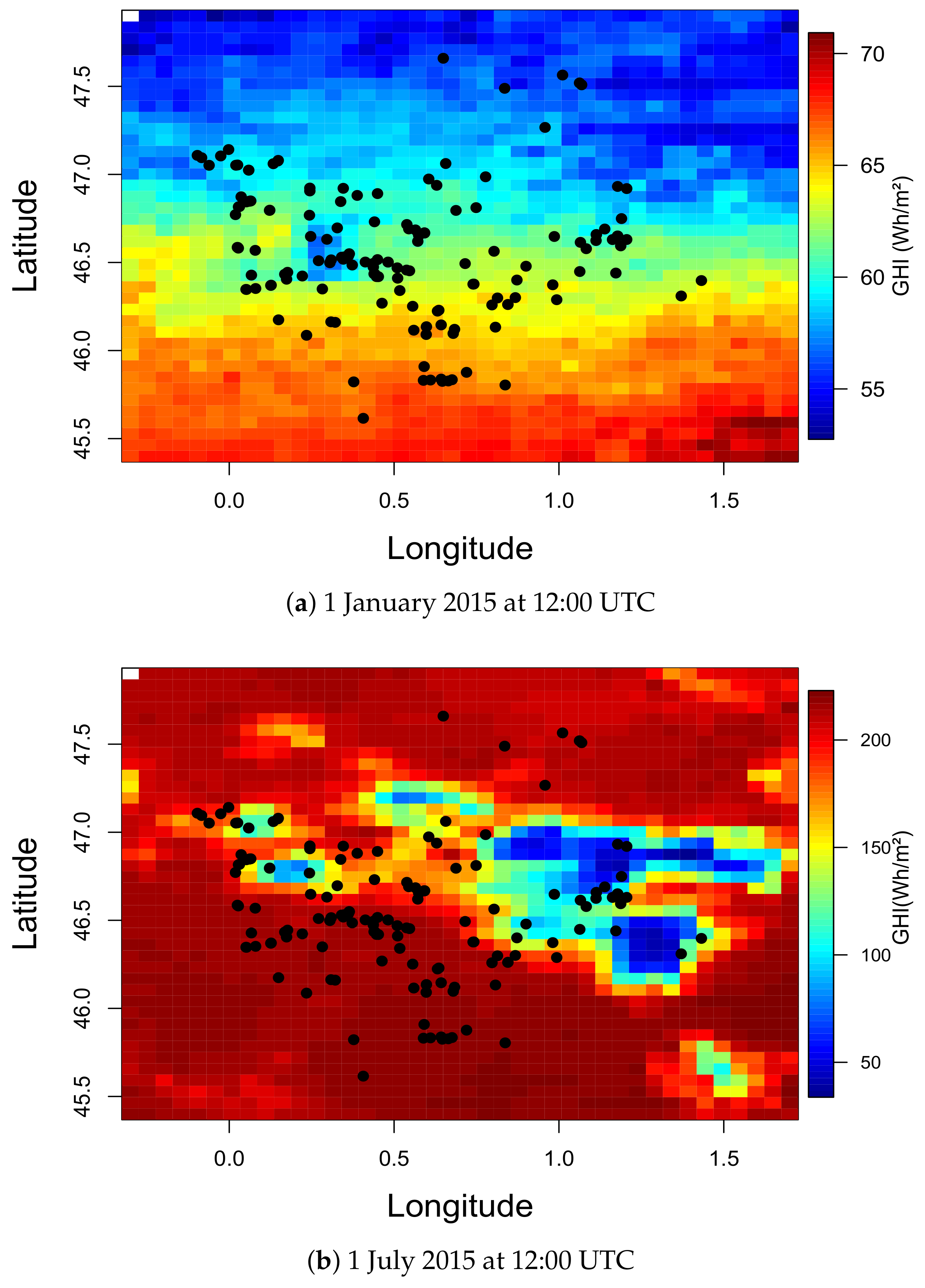
2.2. Satellite Images
3. Proposed Model
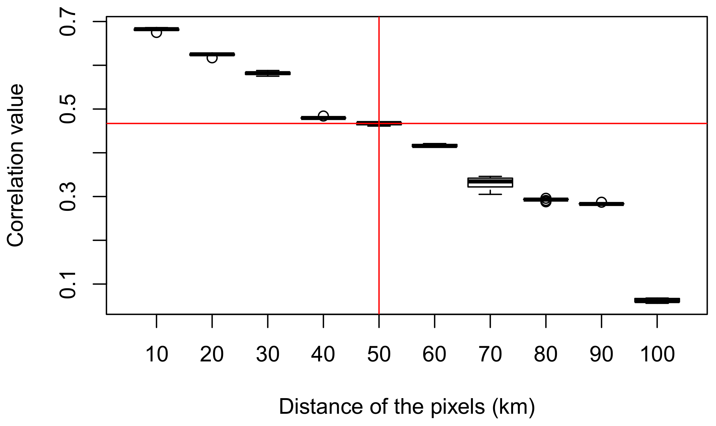
3.1. Identifying the Pixels of Interest
3.2. The Forecasting Model
3.3. Comparison of the Models
- The reference model is the autoregressive model AR which is a model exploiting only the temporal dependencies of the production data only from the site of interest :
- The first model we evaluate is the spatio-temporal model which exploits both temporal dependencies in the measurements but also spatial correlation between measurements of different power plants:
- The second model investigated is an enhancement of the “ST” model with the integration of local meteorological data. This new model is called a spatio-temporal model with conditioning ST(Z) as the parameters are estimated according to the value of the local meteorological variable Z used.
- The last models investigated are the spatio-temporal model which exploits satellite images, NWP forecasts or both.
4. Evaluation of the Forecasts
4.1. Variable Selection and Reduction of Dimension
4.2. Forecasting Performances
- for 15 min horizon, all the models show similar performances;
- for longer horizons the ST model outperforms the AR model;
- the integration of the local meteorological information reduce the MAE compared to when this info is not used;
- the model resulting from the combination of spatio-temporal and satellite data is the best model;
- the use of satellite data in combination with ST measured data results to more efficient forecasts for the short-term forecasting than the combination of ST and NWPs;
- the level of the observed errors is similar to the lowest observed in the literature.
- is the reference AR model
- For each power plants in Table A1 and for each model between the one presented in Section 3.2 (ST, ST(Z), ST+SAT and ST+NWP)
- —
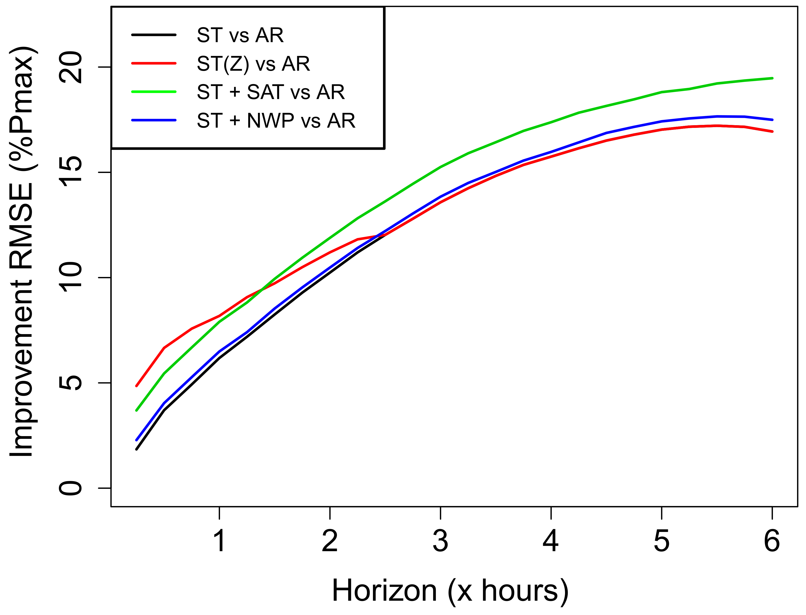
- For each hour of the forecasting horizon, compute on the testing set the RMSE improvement of model over reference model :
- Each line on Figure 8 represents the average improvement at each horizon over all the 9 power plants of a model (over ).

5. Conclusions
Author Contributions
Funding
Data Availability Statement
Acknowledgments
Conflicts of Interest
Abbreviations
| MDPI | Multidisciplinary Digital Publishing Institute |
| DOAJ | Directory of open access journals |
| TLA | Three letter acronym |
| LD | Linear dichroism |
Appendix A. Detailed Evaluation Results

| Power Plant | Criterion | AR | ST | ST(Z) | ST_SAT | ST_NWP |
|---|---|---|---|---|---|---|
| P1 | RMSE | 16.67 | 9.68 | 9.68 | 9.31 | 10.53 |
| MAE | 15.15 | 12.59 | 12.59 | 10.14 | 14.76 | |
| P2 | RMSE | 17.02 | 9.53 | 9.55 | 9.32 | 10.12 |
| MAE | 14.73 | 12.56 | 12.56 | 11.23 | 13.48 | |
| P3 | RMSE | 16.82 | 9.72 | 9.72 | 9.22 | 10.01 |
| MAE | 14.33 | 12.84 | 12.84 | 10.89 | 12.33 | |
| P4 | RMSE | 18.21 | 10.02 | 10.02 | 9.88 | 10.35 |
| MAE | 16.13 | 12.94 | 12.94 | 12.72 | 13.08 | |
| P5 | RMSE | 16.34 | 9.88 | 9.88 | 9.33 | 10.54 |
| MAE | 14.92 | 12.33 | 12.33 | 10.14 | 14.83 | |
| P6 | RMSE | 17.12 | 9.66 | 9.66 | 9.29 | 10.21 |
| MAE | 17.23 | 12.10 | 12.10 | 10.48 | 14.55 | |
| P7 | RMSE | 15.88 | 9.55 | 9.55 | 9.22 | 10.12 |
| MAE | 14.67 | 12.43 | 12.43 | 10.08 | 13.97 | |
| P8 | RMSE | 16.42 | 9.77 | 9.77 | 9.4 | 10.02 |
| MAE | 14.87 | 12.65 | 12.65 | 10.42 | 14.88 | |
| P9 | RMSE | 17.01 | 9.82 | 9.82 | 9.62 | 10.33 |
| MAE | 15.64 | 12.71 | 12.71 | 11.01 | 14.66 |
References
- Kariniotakis, G. Renewable Energy Forecasting: From Models to Applications; Woodhead Publishing: Cambridge, UK, 2017. [Google Scholar]
- Antonanzas, J.; Osorio, N.; Escobar, R.; Urraca, R.; Martinez-de Pison, F.J.; Antonanzas-Torres, F. Review of photovoltaic power forecasting. Sol. Energy 2016, 136, 78–111. [Google Scholar] [CrossRef]
- Sobri, S.; Koohi-Kamali, S.; Rahim, N.A. Solar photovoltaic generation forecasting methods: A review. Energy Convers. Manag. 2018, 156, 459–497. [Google Scholar] [CrossRef]
- Sperati, S.; Alessandrini, S.; Delle Monache, L. An application of the ECMWF Ensemble Prediction System for short-term solar power forecasting. Sol. Energy 2016, 133, 437–450. [Google Scholar] [CrossRef]
- Pierro, M.; Bucci, F.; De Felice, M.; Maggioni, E.; Moser, D.; Perotto, A.; Spada, F.; Cornaro, C. Multi-Model Ensemble for day ahead prediction of photovoltaic power generation. Sol. Energy 2016, 134, 132–146. [Google Scholar] [CrossRef]
- Liu, Y.; Shimada, S.; Yoshino, J.; Kobayashi, T.; Miwa, Y.; Furuta, K. Ensemble forecasting of solar irradiance by applying a mesoscale meteorological model. Sol. Energy 2016, 136, 597–605. [Google Scholar] [CrossRef]
- Alessandrini, S.; Delle Monache, L.; Sperati, S.; Cervone, G. An analog ensemble for short-term probabilistic solar power forecast. Appl. Energy 2015, 157, 95–110. [Google Scholar] [CrossRef]
- Zamo, M.; Mestre, O.; Arbogast, P.; Pannekoucke, O. A benchmark of statistical regression methods for short-term forecasting of photovoltaic electricity production. Part II: Probabilistic forecast of daily production. Sol. Energy 2014, 105, 804–816. [Google Scholar] [CrossRef]
- Nagy, G.I.; Barta, G.; Kazi, S.; Borbély, G.; Simon, G. GEFCom2014: Probabilistic solar and wind power forecasting using a generalized additive tree ensemble approach. Int. J. Forecast. 2016, 32, 1087–1093. [Google Scholar] [CrossRef]
- Huang, J.; Perry, M. A semi-empirical approach using gradient boosting and -nearest neighbors regression for GEFCom2014 probabilistic solar power forecasting. Int. J. Forecast. 2016, 32, 1081–1086. [Google Scholar] [CrossRef]
- Chu, Y.; Coimbra, C.F.M. Short-term probabilistic forecasts for Direct Normal Irradiance. Renew. Energy 2017, 101, 526–536. [Google Scholar] [CrossRef]
- Vagropoulos, S.I.; Kardakos, E.G.; Simoglou, C.K.; Bakirtzis, A.G.; Catalão, J.P.S. ANN-based scenario generation methodology for stochastic variables of electric power systems. Electr. Power Syst. Res. 2016, 134, 9–18. [Google Scholar] [CrossRef]
- Dolara, A.; Grimaccia, F.; Leva, S.; Mussetta, M.; Ogliari, E. A Physical Hybrid Artificial Neural Network for Short Term Forecasting of PV Plant Power Output. Energies 2015, 8, 1138. [Google Scholar] [CrossRef]
- Khodayar, M.; Kaynak, O.; Khodayar, M.E. Rough Deep Neural Architecture for Short-Term Wind Speed Forecasting. IEEE Trans. Ind. Inform. 2017, 13, 2770–2779. [Google Scholar] [CrossRef]
- Noia, M.; Ratto, C.F.; Festa, R. Solar irradiance estimation from geostationary satellite data: I. Statistical models. Sol. Energy 1993, 51, 449–456. [Google Scholar] [CrossRef]
- Noia, M.; Ratto, C.F.; Festa, R. Solar irradiance estimation from geostationary satellite data: II. Physical models. Sol. Energy 1993, 51, 457–465. [Google Scholar] [CrossRef]
- Ineichen, P. Comparison of eight clear sky broadband models against 16 independent data banks. Sol. Energy 2006, 80, 468–478. [Google Scholar] [CrossRef]
- Perez, R.; Moore, K.; Wilcox, S.; Renné, D.; Zelenka, A. Forecasting solar radiation—Preliminary evaluation of an approach based upon the national forecast database. Sol. Energy 2007, 81, 809–812. [Google Scholar] [CrossRef]
- Polo, J.; Wilbert, S.; Ruiz-Arias, J.A.; Meyer, R.; Gueymard, C.; Súri, M.; Martín, L.; Mieslinger, T.; Blanc, P.; Grant, I.; et al. Preliminary survey on site-adaptation techniques for satellite-derived and reanalysis solar radiation datasets. Sol. Energy 2016, 132, 25–37. [Google Scholar] [CrossRef]
- Blanc, P.; Remund, J.; Vallance, L. Short-term solar power forecasting based on satellite images. In Renewable Energy Forecasting; Kariniotakis, G., Ed.; Woodhead Publishing Series in Energy; Woodhead Publishing: Cambridge, UK, 2017; pp. 179–198. [Google Scholar] [CrossRef]
- Peng, Z.; Yu, D.; Huang, D.; Heiser, J.; Kalb, P. A hybrid approach to estimate the complex motions of clouds in sky images. Sol. Energy 2016, 138, 10–25. [Google Scholar] [CrossRef]
- Dong, Z.; Yang, D.; Reindl, T.; Walsh, W.M. Satellite image analysis and a hybrid ESSS/ANN model to forecast solar irradiance in the tropics. Energy Convers. Manag. 2014, 79, 66–73. [Google Scholar] [CrossRef]
- Bosch, J.L.; Kleissl, J. Cloud motion vectors from a network of ground sensors in a solar power plant. Sol. Energy 2013, 95, 13–20. [Google Scholar] [CrossRef]
- Rosiek, S.; Alonso-Montesinos, J.; Batlles, F. Online 3-h forecasting of the power output from a BIPV system using satellite observations and ANN. Electr. Power Energy Syst. 2018, 99, 261–272. [Google Scholar] [CrossRef]
- Linares-Rodriguez, A.; Quesada-Ruiz, S.; Pozo-Vazquez, D.; Tovar-Pescador, J. An evolutionary artificial neural network ensemble model for estimating hourly direct normal irradiances from meteosat imagery. Energy 2015, 91, 264–273. [Google Scholar] [CrossRef]
- Jang, H.S.; Bae, K.Y.; Park, H.S.; Sung, D.K. Solar Power Prediction Based on Satellite Images and Support Vector Machine. IEEE Trans. Sustain. Energy 2016, 7, 1255–1263. [Google Scholar] [CrossRef]
- Wolff, B.; Kühnert, J.; Lorenz, E.; Kramer, O.; Heinemann, D. Comparing support vector regression for PV power forecasting to a physical modeling approach using measurement, numerical weather prediction, and cloud motion data. Sol. Energy 2016, 135, 197–208. [Google Scholar] [CrossRef]
- Mazorra Aguiar, L.; Pereira, B.; David, M.; Díaz, F.; Lauret, P. Use of satellite data to improve solar radiation forecasting with Bayesian Artificial Neural Networks. Sol. Energy 2015, 122, 1309–1324. [Google Scholar] [CrossRef]
- Messner, J.W.; Pinson, P. Online adaptive lasso estimation in vector autoregressive models for high dimensional wind power forecasting. Int. J. Forecast. 2018, 35, 1485–1498. [Google Scholar]
- Dambreville, R.; Blanc, P.; Chanussot, J.; Boldo, D. Very short term forecasting of the Global Horizontal Irradiance using a spatio-temporal autoregressive model. Renew. Energy 2014, 72, 291–300. [Google Scholar] [CrossRef]
- Koster, D.; Minette, F.; Braun, C.; O’Nagy, O. Short-term and regionalized photovoltaic power forecasting, enhanced by reference systems, on the example of Luxembourg. Renew. Energy 2019, 132, 455–470. [Google Scholar] [CrossRef]
- Lorenz, E.; Kühnert, J.; Heinemann, D.; Nielsen, K.P.; Remund, J.; Müller, S.C. Comparison of global horizontal irradiance forecasts based on numerical weather prediction models with different spatio-temporal resolutions. Prog. Photovolt. Res. Appl. 2016, 24, 1626–1640. [Google Scholar] [CrossRef]
- Agoua, X.G.; Girard, R.; Kariniotakis, G. Short-Term Spatio-Temporal Forecasting of Photovoltaic Power Production. IEEE Trans. Sustain. Energy 2018, 9, 538–546. [Google Scholar] [CrossRef]
- Vernay, C.; Blanc, P.; Pitaval, S. Characterizing measurements campaigns for an innovative calibration approach of the global horizontal irradiation estimated by HelioClim-3. Renew. Energy 2013, 57, 339–347. [Google Scholar] [CrossRef]
- Blanc, P.; Gschwind, B.; Lefèvre, M.; Wald, L. The HelioClim Project: Surface Solar Irradiance Data for Climate Applications. Remote Sens. 2011, 3, 343–361. [Google Scholar] [CrossRef]
- Dambreville, R. Nowcasting and Very Short Term Forecasting of the Global Horizontal Irradiance at Ground Level: Application to Photovoltaic Output Forecasting. Ph.D. Thesis, Université de Grenoble, Saint-Martin-d’Hères, France, 2014. [Google Scholar]
- Wartenberg, D. Multivariate Spatial Correlation: A Method for Exploratory Geographical Analysis. Geogr. Anal. 1985, 17, 263–283. [Google Scholar] [CrossRef]
- Agoua, X.G.; Girard, R.; Kariniotakis, G. Probabilistic Model for Spatio-Temporal Photovoltaic Power Forecasting. IEEE Trans. Sustain. Energy 2019, 10, 780–789. [Google Scholar] [CrossRef]


| Horizons | Initial Number of Variables = 1351 | ||
|---|---|---|---|
| Number of Pixels Selected | Number of PV Plants Selected | Total Number of Variables Selected (Lags and Pixels Included) | |
| 15 min | 4 | 28 | 67 |
| 1 h | 4 | 22 | 64 |
| 3 h | 7 | 25 | 56 |
| Metric | Models | ||||
|---|---|---|---|---|---|
| MAE (% Pmax) | AR | ST | ST(Z) | ST + SAT | ST + NWP |
| 15 min | 2.75 | 2.69 | 2.62 | 2.53 | 2.69 |
| 1 h | 5.69 | 5.33 | 5.23 | 4.82 | 5.59 |
| 3 h | 11.81 | 10.21 | 10.21 | 8.66 | 11.61 |
| 6 h | 15.15 | 12.59 | 12.59 | 10.14 | 14.76 |
| Metric | Models | ||||
|---|---|---|---|---|---|
| RMSE (% Pmax) | AR | ST | ST(Z) | ST + SAT | ST + NWP |
| 15 min | 4.32 | 3.12 | 3.00 | 2.90 | 3.34 |
| 1 h | 8.34 | 6.72 | 6.5 | 6.30 | 6.90 |
| 3 h | 10.46 | 8.84 | 8.84 | 8.41 | 9.12 |
| 6 h | 16.67 | 9.68 | 9.68 | 9.31 | 10.53 |
Publisher’s Note: MDPI stays neutral with regard to jurisdictional claims in published maps and institutional affiliations. |
© 2021 by the authors. Licensee MDPI, Basel, Switzerland. This article is an open access article distributed under the terms and conditions of the Creative Commons Attribution (CC BY) license (http://creativecommons.org/licenses/by/4.0/).
Share and Cite
Agoua, X.G.; Girard, R.; Kariniotakis, G. Photovoltaic Power Forecasting: Assessment of the Impact of Multiple Sources of Spatio-Temporal Data on Forecast Accuracy. Energies 2021, 14, 1432. https://doi.org/10.3390/en14051432
Agoua XG, Girard R, Kariniotakis G. Photovoltaic Power Forecasting: Assessment of the Impact of Multiple Sources of Spatio-Temporal Data on Forecast Accuracy. Energies. 2021; 14(5):1432. https://doi.org/10.3390/en14051432
Chicago/Turabian StyleAgoua, Xwégnon Ghislain, Robin Girard, and Georges Kariniotakis. 2021. "Photovoltaic Power Forecasting: Assessment of the Impact of Multiple Sources of Spatio-Temporal Data on Forecast Accuracy" Energies 14, no. 5: 1432. https://doi.org/10.3390/en14051432
APA StyleAgoua, X. G., Girard, R., & Kariniotakis, G. (2021). Photovoltaic Power Forecasting: Assessment of the Impact of Multiple Sources of Spatio-Temporal Data on Forecast Accuracy. Energies, 14(5), 1432. https://doi.org/10.3390/en14051432