A Scalable Real-Time Non-Intrusive Load Monitoring System for the Estimation of Household Appliance Power Consumption

Abstract

Smart-meter technology advancements have resulted in the generation of massive volumes of information introducing new opportunities for energy services and data-driven business models. One such service is non-intrusive load monitoring (NILM). NILM is a process to break down the electricity consumption on an appliance level by analyzing the total aggregated data measurements monitored from a single point. Most prominent existing solutions use deep learning techniques resulting in models with millions of parameters and a high computational burden. Some of these solutions use the turn-on transient response of the target appliance to calculate its energy consumption, while others require the total operation cycle. In the latter case, disaggregation is performed either with delay (in the order of minutes) or only for past events. In this paper, a real-time NILM system is proposed. The scope of the proposed NILM algorithm is to detect the turning-on of a target appliance by processing the measured active power transient response and estimate its consumption in real-time. The proposed system consists of three main blocks, i.e., an event detection algorithm, a convolutional neural network classifier and a power estimation algorithm. Experimental results reveal that the proposed system can achieve promising results in real-time, presenting high computational and memory efficiency.

1. Introduction

Nowadays, the amount of data that is generated almost continuously is enormous. Once analyzed, they can reveal useful information in many different disciplines; economy, healthcare, and e-commerce, to name a few. In this context, the energy sector could not have been an exception. Traditionally, energy data was acquired at a few critical points of the power grid, usually at the transmission level, but the landscape has changed due to the advance in smart-metering technologies. Thousands of internet-of-things (IoT) endpoints are placed within the smart grid, providing energy utilities access to valuable data; thus, new opportunities have been created for energy services and data-driven business models [1,2,3,4,5]. Energy disaggregation is an example of such a service.

Energy disaggregation is the process of consumption breakdown at appliance or activity level for residential or commercial-industrial (C&I) users; in other words, it estimates the individual power consumption for all appliances contributing to the total mains power. This process can help energy utilities reveal useful information to support load forecasting and demand-side management programs. Regarding residential consumers, it can be used to provide accurate billing and meaningful feedback regarding their energy consumption as well as to improve the appliance efficiency (e.g., by detecting old devices and replace them with more efficient ones) [6].

There are two main possible energy disaggregation solutions: (a) Intrusive Load Monitoring (ILM) and (b) Non-Intrusive Load Monitoring (NILM). In ILM, i.e., a hardware-based approach, power meters are attached behind each target appliance. The large number of hardware devices required for ILM makes the installation process difficult and cost-inefficient but results in very accurate power estimates. On the other hand, NILM is a software-based approach. It requires a single meter for the total aggregated power, thus the installation process is simplified and the corresponding cost is reduced. However, since there is no information about the aggregated power appliances, appropriate algorithms should be created to perform energy decomposition.

The utilities should perform a large-scale deployment to support thousands of consumers to benefit as much as possible from energy disaggregation services; only then it is possible to extract useful information for business models. This large-scale deployment makes NILM far more favorable than ILM due to the low cost, installation simplicity and minimum hardware requirements. However, in many cases, NILM algorithms present high computational complexity and significant memory requirements. In this sense, utilities should either use high-end smart meters—or extra hardware attached to them—with powerful central processing units (CPUs) and sufficient memory. Alternatively, energy disaggregation must be performed in cloud services. In the latter case, the cost of cloud services increases with the number of consumers. To this end, utilities must adopt scalable solutions. Scalability can be more critical even than disaggregation accuracy. As it is realized, low computational and memory requirements are necessary to run the service on the edge with conventional microprocessors or minimize the cost of needed cloud services. Furthermore, to improve user experience, minimum feedback must be required; thus, the necessity for pre-trained generic appliance models is of utmost importance.

Several approaches have been proposed to cope with the NILM problem [7,8]. It was first introduced by Hart [9]. Hart’s approach was based on monitoring power changes (corresponding to the appliance turning-on/off events) of both active and reactive power signals. These power changes are grouped into clusters, with each cluster representing a state change of a target appliance. Since then, several works have investigated the NILM problem utilizing different sampling rates and techniques. Earlier approaches employed sampling rates lower than 1 Hz, where event detection (appliances turning-on/off) is impractical and probabilistic models, such as variants of hidden Markov models (HMM) were examined [10,11,12,13,14,15,16,17]. HMMs yield promising results but present disadvantages, e.g., high computational complexity when the number of appliances increases and difficulty in classifying appliances that present similar power consumption [18]. Due to these disadvantages, researchers have turned to alternative methods, including machine learning and deep learning techniques [18,19,20,21,22,23,24,25,26,27,28,29,30,31,32,33,34,35,36,37,38]. NILM approaches can be generally categorized as event-based and state-based.

Event-based solutions [33,34,35,36,37,38,39] leverage the information-rich transient response of an appliance turning-on. Specifically, they consist of two modules: (a) an event detection algorithm for discovering power changes corresponding to an appliance turning-on and (b) a classifier for identifying the appliance that caused the power change. This approach is based on the fact that turn-on transient responses contain more information regarding the operating device than steady states. However, in order to obtain this transient state information, high-resolution data is vital [33,34,35,36,37,38]. One widespread event-based method is the V-I trajectory, utilizing high-resolution voltage and current measurements. In [37,38], useful features are extracted from the V-I trajectories and neural networks are trained for classification. Other researchers depict the trajectories as binary images [34,35,36]. This visual representation solves the appliance recognition problem by exploiting computer vision techniques. Furthermore, transfer learning techniques have been investigated, as in [36] where an image classifier has been implemented based on AlexNet [40]. An important advantage of event-based approaches is the low complexity; only a few time instants corresponding to on/off events are processed. Furthermore, such approaches can detect an appliance turn-on event in real-time since information only from the transient state is required. However, high-resolution data of several kHz is essential, applying mainly to detect appliance turn-on/off events, without calculating power consumption.

On the other hand, state-based approaches [19,20,21,22,23,24,25,26,27] mainly require lower frequency data. These approaches do not detect state transitions. On the contrary, they parse all available data of a time-series, even if no events occur. In such approaches, the appliance must operate for at least some minutes to determine if it is on [20,22]. There are even cases where the appliance end-use has to be fully completed to estimate the power consumption [19,24]. In [19], three different neural network architectures were presented, i.e., (a) long short-term memory (LSTM) networks, (b) stacked denoising autoencoders, and (c) a regression algorithm to forecast the start time, stop time and average power demand of devices. In [21], a bidirectional LSTM cell was used; in [26] a deep convolutional neural network (CNN) that uses as input a time window of active power consumption and predicts the active power in the center of the window. In [23], the authors feed their network with active, reactive, and apparent power and current data. Furthermore, they use mainly CNN blocks in order to create a recurrent property similar to LSTMs. Finally, in [24], an attention-based deep neural network is introduced, inspired by deep learning techniques used in Natural Language Processing (NLP). State-based approaches use low-resolution data and predict the power consumption per appliance. However, they present higher computational complexity since all available data are used, thus cannot detect in real-time an appliance being turned-on/off.

The scope of this paper is to present a real-time event-based NILM methodology to detect an appliance turn-on event and calculate its power consumption in real-time. The proposed NILM design is built on top of three main blocks, i.e., an event detector, a CNN classifier and a power estimation algorithm. The main strengths of the proposed NILM system rely on the following:

• The proposed system can identify when an appliance is turned-on in real-time, based on its active power transient response sampled at 100 Hz; processing data of the total appliance operational duration is not required, as in [19,24].
• The proposed system is delay-free; once the appliance has been turned-on, the system can calculate its power in real-time.
• The combination of a machine learning model to detect appliance turning-on and a heuristic algorithm to estimate the power in real-time constitute a system light-weight, presenting less memory and CPU requirements than end-to-end deep learning models [19,23,24].
• The proposed NILM algorithm is automatic, thus, no feedback is required by the user.
• Data sampling rate of 100 Hz for active power measurements is used, contrary to several kHz in relevant works [33,34,35,41,42].

Generally, as it can be suggested from the above analysis, the proposed system constitutes a real-time scalable solution presenting minimum hardware requirements; thus, it can be integrated into low-cost chip-sets and, consequently, run on the edge.

The paper is structured as follows: In Section 2, the proposed methodology is presented. In Section 3, the dataset and the metrics used for evaluation are described. In Section 4, experimental validation results from real-life installations are analyzed and the performance of the system is compared to other state-of-the-art approaches. In Section 5, an industrial perspective regarding scalable real-time NILM services is discussed. Finally, Section 6 concludes the paper.

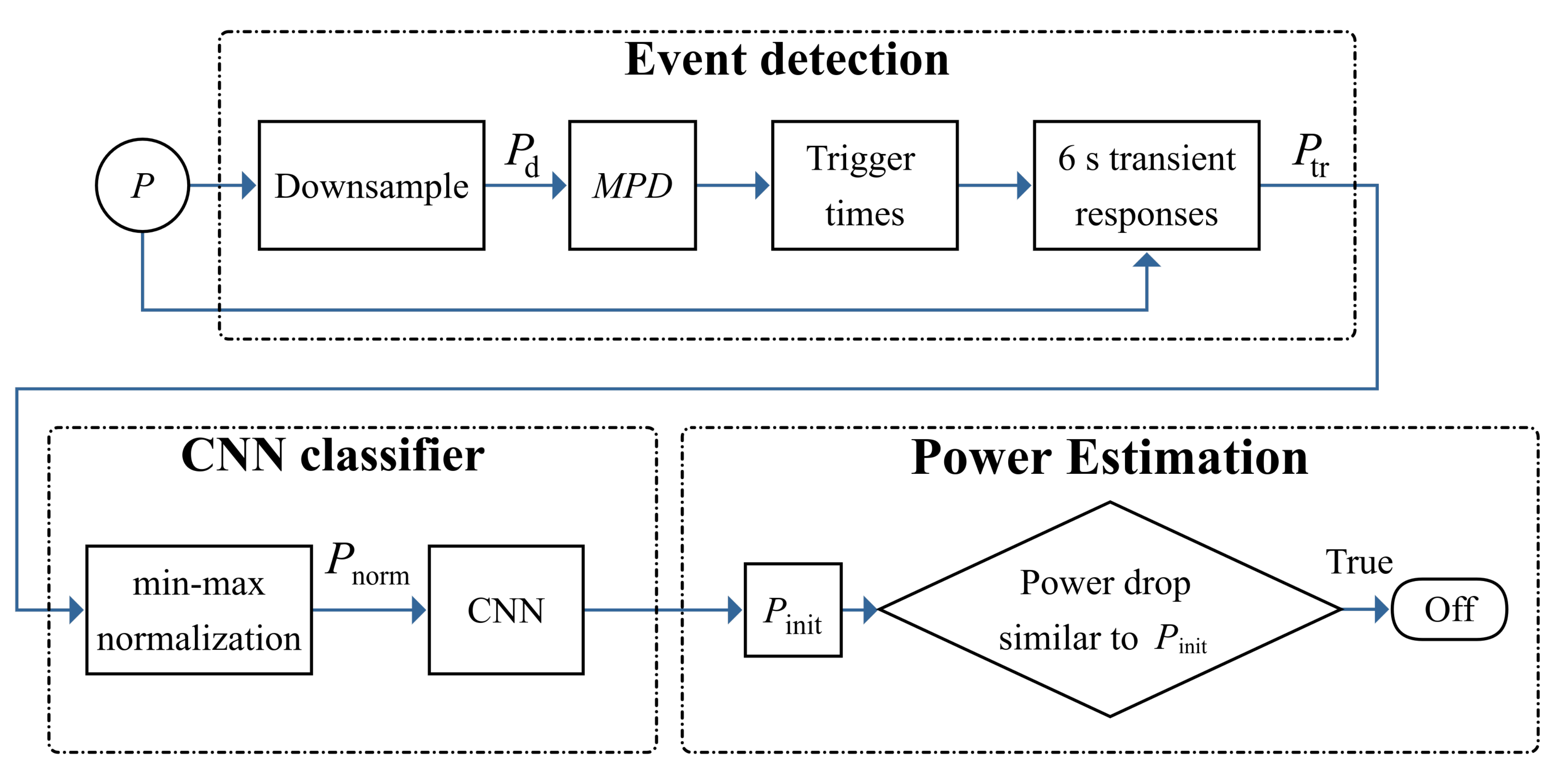
2. Proposed System

The proposed methodology comprises of three main parts: (a) an event-detection system to find active power changes corresponding to turn-on events, (b) a CNN binary classifier to determine if the turn-on event was caused by a specific target appliance or not, and (c) a power estimation algorithm to calculate in real-time the appliance power per second and consequently the energy consumption. An overview of the system in flowchart form is illustrated in Figure 1.

2.1. Event Detection

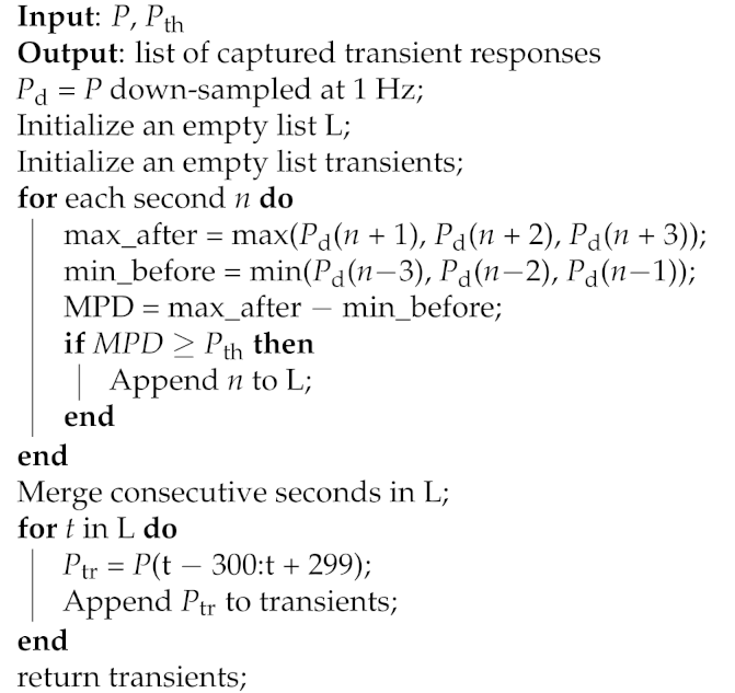
The event detection algorithm is used to identify the time instant (trigger time) when a sudden increase of active power occurs, indicating a possible turn-on event. The advantages of the proposed event detection algorithm are its simplicity and the fact that no pre-training is required.

Let us assume that the aggregated active power time-series at 100 Hz is P. The original signal P is down-sampled at 1 Hz by means of averaging, resulting into signal P_d. Down-sampling is applied for two main reasons: (a) the event detection algorithm becomes simpler, presenting less computational burden and (b) most of power changes are still easily identifiable assuming an 1 Hz sampling frequency. However, if two or more events occur almost simultaneously, e.g., in a period of less than a second, the algorithm detects these events as a single one. Considering that the probability of this scenario is very low, the frequency of 1 Hz has been selected. Next, the maximum power difference (MPD) for each second n is calculated as:

$$MPD\left(n\right)=max(P_d(n+1),P_d(n+2),P_d(n+3))-min(P_d(n-3),P_d(n-2),P_d(n-1)).$$

(1)

MPD shows the maximum difference in active power in a region around n, i.e., the maximum power during the first three seconds after n, minus the minimum power of the three first seconds before n. In this sense, the transient onset can be accurately determined since the real power increase may not appear immediately, but some seconds after n. To determine the trigger time candidates, MPD is compared with a threshold, P_th, which is determined in terms of the appliance rating power. This means that, at time instant n an event occurs if

$$\begin{array}{c}\hfill MPD\left(n\right)>P_{th}.\end{array}$$

(2)

At this point, it should be mentioned that trigger time candidates close in time are merged. For each trigger time, a 6 s window of the captured transient response, P_tr, is generated from P (100 × 6 = 600 samples). The pseudo-code for the process described is presented in Algorithm 1.

Algorithm 1: Event detection.

2.2. CNN Classifier

In the proposed methodology, the transient response generated by an appliance’s turning-on is used as the load signature for appliance classification [7]. Whenever a target appliance is turned on, a transient response can be detected in the aggregated active power waveform. Besides appliance classification, this load signature presents two additional advantages. Firstly, for a given appliance, the turn-on transient response pattern is unique and relates only to the operational characteristics of the appliance [43]. Consequently, the identification algorithm’s performance is independent of the simultaneous operation of other types of appliances, even when a large number of devices is considered [7,44]. Secondly, the proposed algorithm can successfully treat various types of appliances, even though presenting similar consumption levels at steady-state, since classification is performed based on the unique appliance transient characteristics instead of calculating steady-state features.

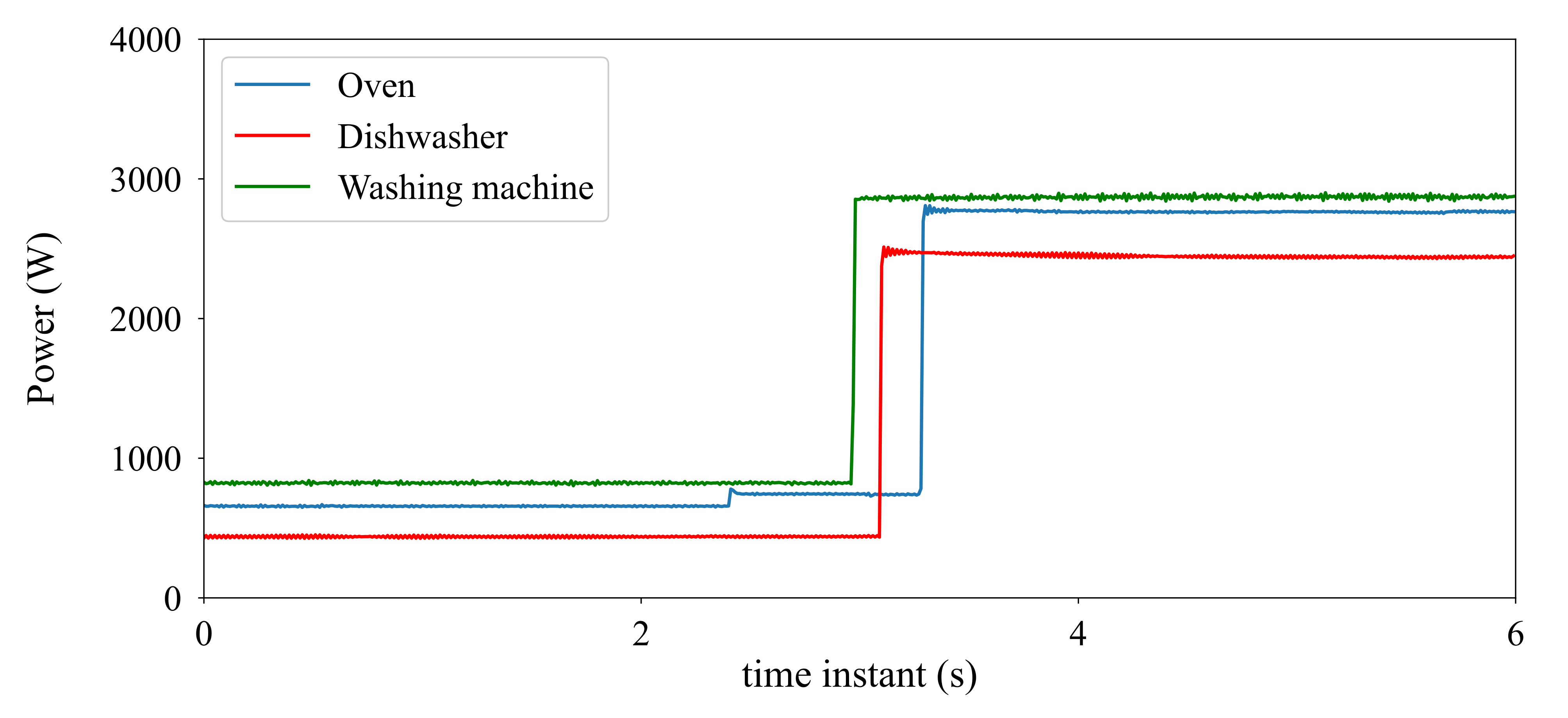
The same principle can detect specific operational states by identifying transient responses caused by a state transition regarding multi-state appliances. For example, for a washing machine or a dishwasher, the water heating process’s transient response can be used to identify this specific state, being of primary interest as the most energy-intensive process during an operation cycle.

In order to associate a given transient response, P_tr, with a specific target appliance behavior, a CNN classifier is utilized. In this sense, for each target appliance, a dedicated CNN classifier is used, identifying P_tr as positive when related to the target appliance or negative otherwise.

Different types of appliances generate transient responses with distinct characteristics, primarily when a high sampling frequency, e.g., at 100 Hz, is used. Suppose a user was initially given an example of such a response corresponding to a specific appliance. In that case, he/she could later recognize a new response of the same appliance by simple visual inspection. However, the implementation of such a recognition algorithm is not an easy task.

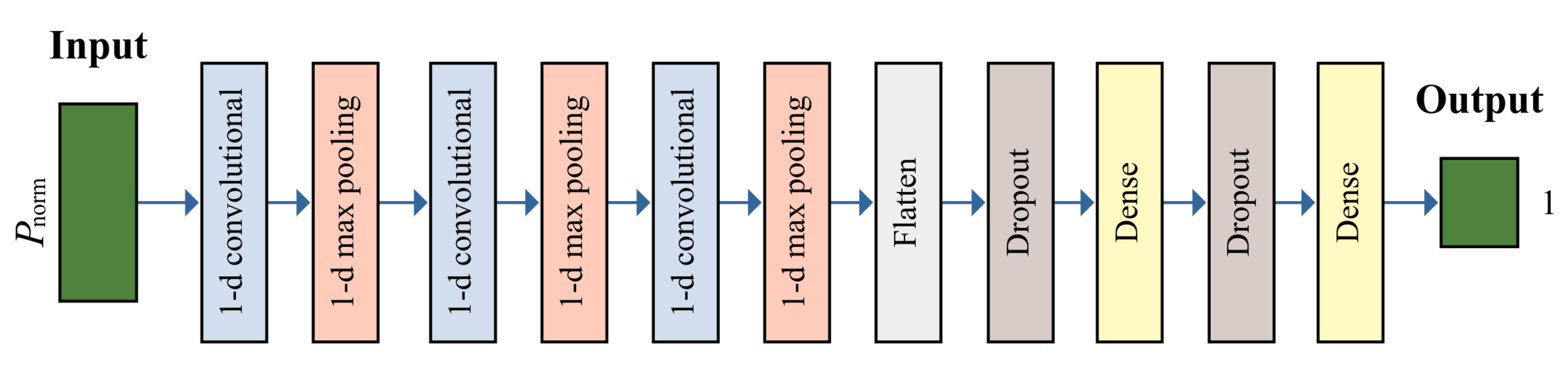
Inspired from the area of computer vision, where CNN models are used for image recognition, and classification [45], a similar approach has been adopted in this paper. Convolutional layers can automatically extract useful features from the input data without user supervision [45]. Thus, there is no need to implement specific algorithms; instead, by training a CNN model, the classification problem can be successfully solved. A block diagram of the proposed CNN architecture is depicted in Figure 2.

Initially, min-max normalization is applied to P_tr by means of (3); the resulting normalized vector, P_norm, is forwarded as input to the CNN model.

$$P_{\mathrm{norm}}=\frac{P_{tr}-min\left(P_{tr}\right)}{max\left(P_{tr}\right)-min\left(P_{tr}\right)}$$

(3)

Since the CNN input model is an one-dimensional signal, one-dimensional convolutional layers are used to extract the useful features from P_norm. In particular, three consecutive 1-d convolutional layers are used in combination with an 1-d max-pooling layer. All convolutional layer parameters have been set to 32 filters, kernel size equal to 3, strides equal to 1, ’same’ padding, and rectified linear unit (ReLU) activation function. The ReLU function is defined as

$$\mathrm{ReLU}\left(\mathrm{x}\right)=max(\mathrm{x},0)$$

(4)

for $x\in \mathbb{R}$. For max-pooling layers, the pool size was set to 2. Generally, at each 1-d convolutional layer, a number of filters is applied to the corresponding input, x_conv. Assuming that the size of x_conv is $M_{\mathrm{conv}}\times N_{\mathrm{conv}}$ and a single filter, f, is of $3\times N_{\mathrm{conv}}$, the output of the convolution between x_conv and f will be a $M_{\mathrm{conv}}\times 1$ matrix. The resulting y_conv is calculated as

$${\mathbf{y}}_{conv}\left(m\right)=max{(}\sum _{t=1}^3\sum _{n=1}^{N_{\mathrm{conv}}}{\mathbf{x}}_{conv}(m+t-2,n)\mathbf{f}(t,n),0{)}$$

(5)

for $m\in [1,\dots ,M_{\mathrm{conv}}]$, where x_conv(0, n) and x_conv(M_conv+1, n) are considered zero for any $n\in [1,\dots ,N_{\mathrm{conv}}]$ as a result of zero-padding. In our case, where 32 filters are used in a convolutional layer results y_conv, are stacked as columns, forming a $M_{\mathrm{conv}}\times 32$ matrix.

Each layer is followed by a max-pooling layer to down-sample the extracted features of the input signal. In this sense, a summarized version of the extracted features (half the size) is created, maintaining the most important features and is further used as input to the next layer. Assuming x_pool, with size $M_{\mathrm{pool}}\times N_{\mathrm{pool}}$ is the max-pooling layer input matrix, the output, y_pool, has a size of $(M_{\mathrm{pool}}/2)\times N_{\mathrm{pool}}$ and is calculated as

$${\mathbf{y}}_{pool}(m,n)=max({\mathbf{x}}_{pool}(2m-1,n),{\mathbf{x}}_{pool}(2m,n))$$

(6)

for $m\in [1,\dots ,M_{\mathrm{pool}}/2]$ and $n\in [1,\dots ,N_{\mathrm{pool}}]$.

Following the three convolutional/pooling pairs, a flattening layer is applied, transforming its input to a single vector by column-wise stacking. Finally, two dense layers are used of 20 and 1 output nodes, respectively. For the first dense layer, the ReLU activation function is applied; for the last layer, the sigmoid activation function defined in (7) for $x\in \mathbb{R}$ is used to compute the probability of the transient response to correspond to the positive class.

$$\mathrm{S}\left(\mathrm{x}\right)=\frac{1}{1+{\mathrm{e}}^{-\mathrm{x}}}$$

(7)

Generally speaking, a dense layer with $M_{\mathrm{dense}}$ input nodes and K output nodes includes two trainable parameters, i.e., a weight matrix, w, with size $M_{\mathrm{dense}}\times K$ and a bias vector, b, with size K. Given an input vector, x_dense, with $M_{\mathrm{dense}}$ elements, the output y_dense of size K is calculated as

$${\mathbf{y}}_{dense}\left(k\right)=F(\sum _{m=1}^{M_{\mathrm{dense}}}{\mathbf{x}}_{dense}\left(m\right)\mathbf{w}(m,k)+\mathbf{b}\left(k\right))$$

(8)

for $k\in [1,\dots ,K]$, where F is the corresponding activation function. Before each dense layer, a dropout layer [46] is used. Its value is set to 0.2 to prevent model over-fitting.

A standard backpropagation algorithm is used during training to optimize the binary cross-entropy loss between the predicted probabilities and the actual labels. Assuming that the predicted probabilities are $p_1,p_2,\dots ,p_B$ for B samples and the actual labels are $q_1,q_2,\dots ,q_B$, the binary cross-entropy loss is

$$L=-\frac{1}{B}\sum _{b=1}^B{[}{q}_b{log}_2{p}_b+(1-q_b){log}_2(1-p_b){]}.$$

(9)

The CNN classifier is trained for a maximum of 50 iterations. The Adamax optimizer [47] was selected assuming an initial learning rate of 0.01 and batch size 32. In order to avoid over-fitting, early stopping with patience is used. The training process stops once the validation accuracy does not improve after five consecutive iterations.

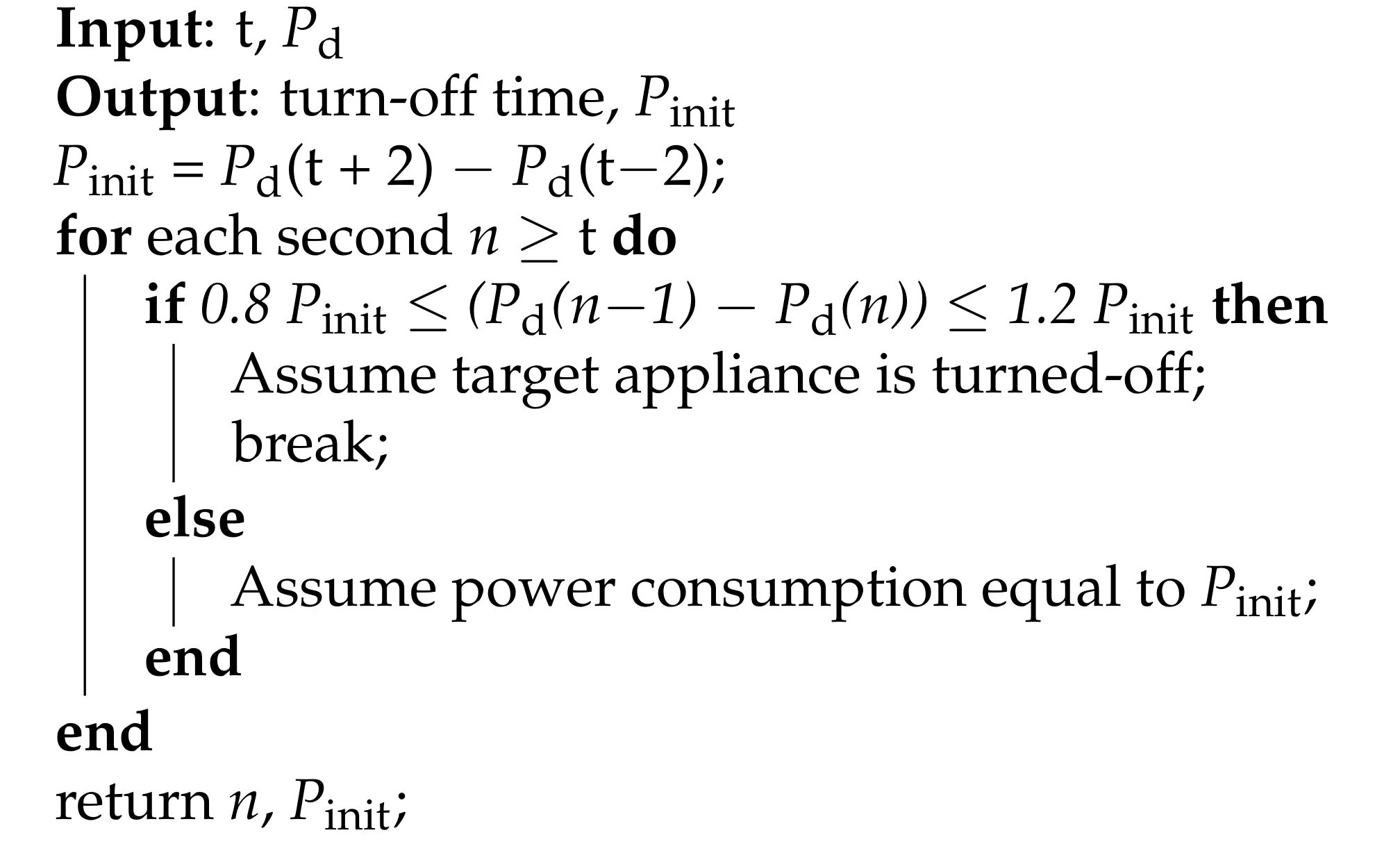
2.3. Consumed Energy Estimation Algorithm

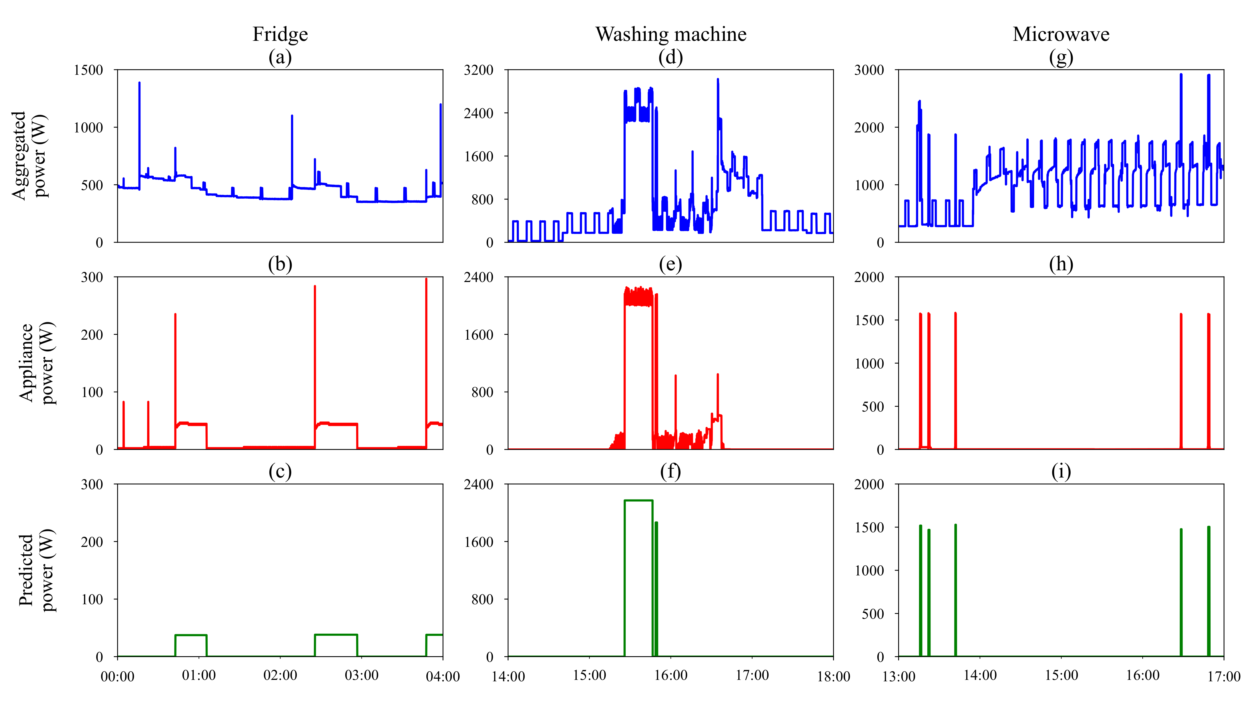
The last module is related to the real-power estimation of the target appliance. The implemented algorithm considers the appliance end-uses as pulses of constant power; this approximation is well-suited for single-state appliances such as microwave oven, kettle or toaster. In the case of appliances with operating cycles comprising of multiple pulses, the algorithm considers each pulse as a new appliance end-use and not as a single end-use event of several pulses. An example is the oven turning-on and off controlled by a thermostat and the dishwasher, where several water heating pulses may occur depending on the selected program. In this sense, the proposed algorithm performance may degrade for multi-state appliances. They are characterized by varying power consumption and cannot be approximated with a constant power pulse. However, such appliances present a predominant energy-intensive process during a full operating cycle while the rest operating states are less critical regarding the total energy consumption. For example, washing machine or dishwasher cycles include energy-intensive water heating processes and low energy-consuming processes, e.g., water pumping. Therefore, regarding multi-state appliances, the proposed power estimation algorithm focuses on the estimation of the energy-intensive processes neglecting the effect of the minor consuming ones.

When the CNN classifies a transient response as positive, it is implied that the appliance has been turned-on. The calculated power increase, P_init is considered equal to the appliance power consumption and assumed constant during the total time of operation of the appliance. When a power decrease between two consecutive seconds in P_d inside the interval [0.8 P_init, 1.2 P_init] is detected, the appliance is considered to be turned-off. The pseudo-code of the energy consumption estimation algorithm is shown in Algorithm 2, having as input the time (in seconds), t, when the target appliance is turned-on and P_d.

Algorithm 2: Energy consumption estimation.

3. Evaluation Methodology

3.1. Dataset

The proposed NILM system is based on the fact that each household appliance presents a transient response pattern with distinct characteristics, becoming more noticeable as the sampling frequency increases. In this paper, the selected sampling frequency is 100 Hz; at this frequency the transient characteristics are captured in contrast to lower sampling rates where such information may be lost. In Figure 3, turn-on transient responses at 100 Hz and 1 Hz for five appliances are depicted. It is evident that the frequency of 100 Hz reveals unique details that are lost when sampling at 1 Hz. More specifically, Figure 3a presents the turn-on response of a high-power consumption (~1.2 kW) fridge compressor with a duration of fewer than two seconds. Figure 3b visualizes the water heating process of a washing machine, which corresponds to a steep power step-up. Next, Figure 3c illustrates the transient response of a microwave oven as a high-power spike followed by a smooth power increase. In Figure 3d, a stove turn-on presenting a smooth and convex power increase is shown, and finally, in Figure 3e visualizes the transient response from a heat pump dryer appliance, including a high-power spike at motor starting time.

An extensive set of transient responses for each target appliance is required to train the CNN classifier. For this purpose, a private dataset that includes transient responses of different household appliances sampled at 100 Hz from different installations is used. The type of appliance and the number of samples for each case are summarized in

Table 1. Private dataset: Number of transient responses for the appliances of interest.

Appliance	Number of Transient Responses
Fridge	132
Dishwasher	171
Heat pump	202
Washing machine	135
Oven	82
Stove	148
Heat pump dryer (drum spinning)	54
Heat pump dryer (heating)	42
Microwave	290

. Note that, the duration of the transient responses contained in the dataset ranges from 12 s to 1 min.

2

In this study, three appliances are selected to test the proposed methodology’s performance, i.e., fridge, washing machine, and microwave oven. Pulses can approximate the end-use of these appliances without significant error in power estimation. Furthermore, such appliances are considered typical for most households, corresponding to substantial total energy consumption. The selected appliances represent a larger group of appliances since both single-state and multi-state appliances are considered. Additionally, detailed results regarding the analysis of such appliances can be found in several relevant works [19,20,22,25,26,27]; thus, a comprehensive comparative analysis can be performed. Finally, low energy-consuming appliances such as game consoles and phone chargers have not been investigated, being of trivial importance and hard to be identified in terms of NILM algorithm application [19].

For each target appliance, a binary classifier is implemented and trained. During training, the transient responses of the appliance under consideration are labeled positive; the responses corresponding to a different appliance are labeled negative. Balancing of the positive and negative classes is performed in order to prevent bias towards the class with the most samples; the number of negative responses is the same as the number of positive ones. A training/validation/testing split is used assuming a ratio of 60%/20%/20% to avoid over-fitting for each class separately.

However, because the number of samples per appliance is small, augmentation techniques are used. These techniques aim to increase the number as well as the diversity of the training samples by artificially introducing variations in existing transient responses. Specifically, for each transient response, 15 samples with the required length of 6 s are created. Assuming that the time-series that contains a response is z, each one of the 15 samples is generated by means of the following steps:

• Considering that the transient response starts at index s of z, a random number u in the interval [s − 500, s − 100] is selected, following uniform distribution. The selected sample is equal to z from index u to index u + 599.
• White Gaussian noise with mean value (μ) equal to 0 and standard deviation (σ) equal to 1 is added to the sample; 10 W maximum power is considered.

The number of samples for training, validation and testing the sets per appliance is shown in

Table 2. Number of positive samples per set.

Appliance	Training	Validation	Testing
Fridge	2400	780	780
Washing machine	2430	810	810
Microwave	5220	1740	1740

.

3.2. Performance Metrics

The proposed methodology is evaluated in terms of the event detection algorithm, the CNN classifiers as well as the overall system performance. For each case, different metrics are used.

3.2.1. Metrics for Event Detection Evaluation

For the event detection algorithm the true positive rate ($TPR=TP/(TP+FN)$), the false positive rate ($FPR=FP/(FP+TN)$) and false negative rate ($FNR=FN/(TP+FN)$) are calculated; TP, FN, FP and TN are the number of true positives, false negatives, false positives and true negatives, respectively. Here, a sample (a time instant) is positive if it is an actual event (there is an appliance turning-on or off) and negative if not.

3.2.2. Metrics for Classifier Evaluation

To evaluate the classifier, the most common metrics used in classification and NILM problems are adopted [18,29,32,34,35]. Specifically, the accuracy, precision, recall and F₁-score, defined in (10)–(13), respectively, are calculated

$$accuracy={\displaystyle \frac{TP+TN}{TP+TN+FP+FN}}$$

(10)

$$precision={\displaystyle \frac{TP}{TP+FP}}$$

(11)

$$recall={\displaystyle \frac{TP}{TP+FN}}$$

(12)

$$F_1=2·{\displaystyle \frac{precision·recall}{precision+recall}}.$$

(13)

In this context, for a transient response classifier, a sample (i.e., transient response of 6 s) is positive if the transient response corresponds to the target appliance. Otherwise, it is assumed negative.

3.2.3. Metrics for Overall NILM System Evaluation

The overall proposed NILM system is tested by using the same metrics as previously, i.e., accuracy, precision, recall, and F₁-score to evaluate the predicted status of the appliance (ON or OFF). Thus, a sample (i.e., a time instant) is considered positive if the appliance is ON and negative if not. It should be mentioned that an appliance is considered turned-on if the measured active power is higher than 5 W. Additionally, for energy estimation, the mean absolute error (MAE) and the root mean square error (RMSE) in (14) and (15), respectively, are computed

$$MAE=\frac{1}{N}\sum _{n=1}^N|y\left[n\right]-\widehat{y}\left[n\right]|$$

(14)

$$RMSE=\sqrt{{\displaystyle \frac{1}{N}}\sum _{n=1}^N{(y\left[n\right]-\widehat{y}\left[n\right])}^2}$$

(15)

where y[n] and ŷ[n] is the original and the estimated power response with N samples. Moreover, the relative error in total energy (RE), defined in (16), is calculated

$$RE=\frac{|E-\widehat{E}|}{max(E,\widehat{E})}$$

(16)

where E and Ê is the original and the estimated total energy consumption of the appliance.

4. Results

In this section, experimental validation results are analyzed considering data from real-world installations. The Building-Level fully-labeled dataset for Electricity Disaggregation (BLUED) [48] is used to test the applicability of the proposed event-detection algorithm. Energy consumption data from three household installations are also used to evaluate the performance of the proposed methodology; common metrics are employed and results are compared with those obtained from other state-of-the-art methods proposed in the literature. Finally, the computational and memory efficiency of the proposed system is discussed.

4.1. Event Detection Evaluation

The BLUED dataset contains aggregate voltage/current and active power data, sampled at 12 kHz and 60 Hz, respectively, from a 2-phase household in Pittsburgh, USA. The recording duration is eight days. The time instants when a turn-on or turn-off event occurred are also reported in the dataset. In particular, for testing the proposed event-detection algorithm, the active power measurements of phase A, at 1 Hz, from 11:58:32 20 October 2011, to 09:29:55 21 October 2011, are used. In fact, during this period, 125 events have occurred, including six pairs of simultaneous events. The proposed algorithm detects the simultaneous events as well as two near-simultaneous turn-off events as single events, respectively. Finally, one false event is detected; an appliance power drop, was incorrectly identified as an appliance turning-off, while the appliance being still in operation. In summary, 118 out of the 125 events have been correctly detected by the proposed event-detection algorithm. In Figure 4, the active power and the detected events for the period from 18:30:00 to 20:30:00 are shown.

The TPR, FPR and FNR metrics are calculated and compared to other more complex solutions [32,49,50] in

Table 3. Event detection evaluation.

Reference	TPR	FPR	FNR
Proposed	94.400%	0.003%	5.600%
[32]	94.000%	0.088%	6.000%
[49]	96.700%	0.810%	3.300%
[50]	94.130%	0.260%	5.870%

. It can be seen that the proposed algorithm can achieve good results while being simple and computationally efficient.

4.2. Classification Evaluation

To evaluate the classifiers performance regarding the three target appliances, the private testing sets mentioned in Section 3.1 are used. The calculated accuracy, precision, recall and F₁-score results are summarized in

Table 4. Classification results.

Appliance	Accuracy	Precision	Recall	F1-Score
Fridge	0.978	0.984	0.972	0.978
Washing machine	0.872	0.875	0.867	0.871
Microwave	0.992	0.986	0.999	0.992

.

It is evident that the proposed classification algorithm presents high performance regarding the microwave and the fridge. These appliances are related to transient response patterns presenting specific characteristics, thus can be identified with high confidence. However, this is not the case for the washing machine, since the turn-on transient response is a simple steep step-up waveform. Similar patterns are also related to the heating processes of most of the household appliances, e.g., dishwasher, oven and generally appliances that use resistive elements for heating as shown in Figure 5. This illustrates the relatively lower scores obtained for the washing machine metrics compared to the other appliances.

4.3. Application on Residential Households

The overall performance of the proposed methodology is tested on a private dataset. This dataset includes three 3-phase power supply households located in the Netherlands. For each household, aggregated active power per phase was measured at 100 Hz along with power consumption of selected appliances for 15 days. For evaluation purposes, the proposed NILM system is applied only when the target appliance is connected.

Figure 6 presents the results for each target appliance, assuming an operational duration of four hours. Specifically, the aggregated power is colored in blue. The actual target appliance power measured with plugwise meters is colored in red. The target appliance power, as estimated by the proposed methodology, is colored in green.

The accuracy, precision, recall, F₁-score, MAE, RMSE and RE are calculated as well as their average considering the three households for 15 days. Results for the fridge, washing machine and microwave oven are shown in

Table 5. Results for fridge.

House	Accuracy	Precision	Recall	F1-Score	MAE (W)	RMSE (W)	E (kWh)	$\hat{\mathit{E}}$ (kWh)	RE
1	0.86	0.94	0.77	0.85	12.97	38.67	14.26	11.74	0.18
2	0.89	0.96	0.74	0.84	7.05	17.14	6.19	4.24	0.32
3	0.98	1.00	0.90	0.95	3.68	12.89	4.74	5.05	0.06
Average	0.91	0.97	0.80	0.88	7.90	22.90	-	-	0.19

,

Table 6. Results for washing machine.

House	Accuracy	Precision	Recall	F1-Score	MAE (W)	RMSE (W)	E (kWh)	$\hat{\mathit{E}}$ (kWh)	RE
1	0.94	0.99	0.24	0.39	20.86	168.96	19.85	12.83	0.35
2	0.97	0.94	0.24	0.38	10.02	116.83	10.44	8.44	0.19
3	0.93	0.42	0.13	0.20	24.27	183.42	7.27	12.61	0.42
Average	0.95	0.78	0.20	0.32	18.38	156.40	-	-	0.32

and

Table 7. Results for microwave.

House	Accuracy	Precision	Recall	F1-Score	MAE (W)	RMSE (W)	E (kWh)	$\hat{\mathit{E}}$ (kWh)	RE
1	1.00	0.94	0.52	0.67	1.28	36.55	2.16	2.13	0.01
2	1.00	0.99	0.46	0.63	1.08	37.63	2.10	1.90	0.10
3	0.99	0.82	0.47	0.60	2.61	57.27	2.19	2.57	0.15
Average	1.00	0.92	0.48	0.63	1.66	43.82	-	-	0.09

, respectively. It can be generally observed that the proposed algorithm presents high accuracy regarding the power and energy estimates of the fridge and the microwave. On the contrary, the microwave oven recall metric is low. This can be attributed to the fact that the proposed methodology considers this appliance standby mode of operation as OFF. In fact, the power consumption during this period is low, thus, of trivial importance regarding energy consumption calculations. Regarding the washing machine results, the NILM system is designed to detect only the most energy-intensive process during the washing machine operation cycle, i.e., water heating mode of operation. For the rest of the operational cycles (non-detected), i.e., water pumping, drum spinning, rinsing, the appliance status is assumed OFF. The partial detection of the washing machine appliance is evident in Figure 6, resulting into low recall scores. Moreover, in the third household, the calculated low precision is due to the operation of appliances presenting similar transient response patterns, being misclassified as washing machine end-uses.

4.4. Comparison with Other Methods

The performance of the proposed methodology is compared to other NILM-based energy consumption estimation systems. The average MAE, RE, precision, recall, F₁-score and accuracy calculations obtained by the proposed method are summarized in

Table 8. Comparison results among existing non-intrusive load monitoring (NILM) solutions for fridge identification and energy consumption estimation.

Reference	Method	Sampling Frequency	Dataset	MAE	RE	Precision	Recall	F1-Score	Accuracy
Proposed		100 Hz	private	7.90	0.19	0.97	0.80	0.88	0.91
[19]	Autoencoder	0.167 Hz	UK-DALE	26.00	0.38	0.85	0.88	0.87	0.90
[19]	CNN	0.167 Hz	UK-DALE	18.00	0.13	0.79	0.86	0.82	0.87
[19]	LSTM	0.167 Hz	UK-DALE	36.00	0.25	0.72	0.77	0.74	0.81
[20]	LSTM	0.167 Hz	UK-DALE	51.00	0.21	0.45	0.51	0.47	0.60
[20]	GRU	0.167 Hz	UK-DALE	51.00	0.26	0.46	0.75	0.57	0.60
[20]	seq2point	0.167 Hz	UK-DALE	51.00	0.29	0.42	0.74	0.53	0.54
[21]	LSTM	0.333 Hz	REDD	-	-	0.91	0.96	0.93	-
[22]	WGRU	0.167 Hz	UK-DALE	28.46	0.13	-	-	0.82	-
[22]	SAEDdot	0.167 Hz	UK-DALE	35.25	0.60	-	-	0.62	-
[22]	SAEDadd	0.167 Hz	UK-DALE	32.31	0.65	-	-	0.66	-
[25]	PCNN AE	0.167 Hz	UK-DALE	3.46	-	-	-	-	-
[25]	PCNN LSTM	0.167 Hz	UK-DALE	3.22	-	-	-	-	-
[26]	seq2seq	0.167 Hz	UK-DALE	24.49	-	-	-	-	-
[26]	seq2point	0.167 Hz	UK-DALE	20.89	-	-	-	-	-
[27]	UNet	0.167 Hz	UK-DALE	15.12	-	-	-	-	-

Note: GRU stands for gated recurrent units, seq2point/seq2seq for sequence-to-point/sequence-to-sequence, WGRU for window GRU, SAEDdot/SAEDadd for self-attentive energy disaggregation with ‘additive’/‘dot’ attention mechanism, PCNN AE for parallel CNN autoencoder.

,

Table 9. Comparison results among existing NILM solutions for washing machine identification and energy consumption estimation.

Reference	Method	Sampling Frequency	Dataset	MAE	RE	Precision	Recall	F1-score	Accuracy
Proposed		100 Hz	private	18.38	0.32	0.78	0.20	0.32	0.95
[19]	Autoencoder	0.167 Hz	UK-DALE	24.00	0.48	0.07	1.00	0.13	0.82
[19]	CNN	0.167 Hz	UK-DALE	11.00	0.74	0.29	0.24	0.27	0.98
[19]	LSTM	0.167 Hz	UK-DALE	109.00	0.91	0.01	0.73	0.03	0.23
[20]	LSTM	0.167 Hz	UK-DALE	25.00	0.35	0.16	0.56	0.24	0.95
[20]	GRU	0.167 Hz	UK-DALE	30.00	0.58	0.22	0.54	0.31	0.96
[20]	seq2point	0.167 Hz	UK-DALE	17.00	0.28	0.26	0.55	0.35	0.97
[22]	WGRU	0.167 Hz	UK-DALE	10.45	0.43	-	-	0.34	-
[22]	SAEDdot	0.167 Hz	UK-DALE	13.10	0.34	-	-	0.30	-
[22]	SAEDadd	0.167 Hz	UK-DALE	22.01	0.53	-	-	0.30	-
[25]	PCNN AE	0.167 Hz	UK-DALE	83.40	-	-	-	-	-
[25]	PCNN LSTM	0.167 Hz	UK-DALE	73.16	-	-	-	-	-
[26]	seq2seq	0.167 Hz	UK-DALE	10.15	-	-	-	-	-
[26]	seq2point	0.167 Hz	UK-DALE	12.66	-	-	-	-	-
[27]	UNet	0.167 Hz	UK-DALE	11.51	-	-	-	-	-

and

Table 10. Comparison results among existing NILM solutions for microwave identification and energy consumption estimation.

Reference	Method	Sampling Frequency	Dataset	MAE	RE	Precision	Recall	F1-Score	Accuracy
Proposed		100 Hz	private	1.66	0.09	0.92	0.48	0.63	1.00
[19]	Autoencoder	0.167 Hz	UK-DALE	9.00	0.73	0.15	0.94	0.26	0.99
[19]	CNN	0.167 Hz	UK-DALE	6.00	0.50	0.14	0.40	0.21	0.99
[19]	LSTM	0.167 Hz	UK-DALE	20.00	0.88	0.07	0.99	0.13	0.98
[20]	LSTM	0.167 Hz	UK-DALE	86.00	0.10	0.01	0.45	0.02	0.93
[20]	GRU	0.167 Hz	UK-DALE	97.00	0.07	0.02	0.75	0.04	0.93
[20]	seq2point	0.167 Hz	UK-DALE	103.00	0.16	0.01	0.79	0.03	0.91
[21]	LSTM	0.333 Hz	REDD	-	-	0.50	0.05	0.09	-
[22]	WGRU	0.167 Hz	UK-DALE	4.36	0.25	-	-	0.44	-
[22]	SAEDdot	0.167 Hz	UK-DALE	5.97	0.19	-	-	0.25	-
[22]	SAEDadd	0.167 Hz	UK-DALE	5.98	0.17	-	-	0.26	-
[25]	PCNN AE	0.167 Hz	UK-DALE	27.50	-	-	-	-	-
[25]	PCNN LSTM	0.167 Hz	UK-DALE	9.42	-	-	-	-	-
[26]	seq2seq	0.167 Hz	UK-DALE	13.62	-	-	-	-	-
[26]	seq2point	0.167 Hz	UK-DALE	8.67	-	-	-	-	-
[27]	UNet	0.167 Hz	UK-DALE	6.48	-	-	-	-	-

regarding the fridge, washing machine and microwave, respectively. The corresponding results (where available) reported in the relevant literature are also presented as well as the associated NILM technique, sampling frequency, and testing dataset. Note that, most of the literature state-of-the-art methods have been tested by using the well-known UK Domestic Appliance-Level Electricity (UK-DALE) [51] dataset. This dataset includes aggregated active power and appliance measurements of 0.167 Hz for several months, recorded for a small number of household installations. Moreover, the Reference Energy Disaggregation Data Set (REDD) [52] has been used in [21] to evaluate the LSTM algorithm performance; the sampling frequency is 1 Hz for mains and 0.333 Hz for the appliances. The proposed NILM system is tested by using an 100-Hz private dataset, since high-frequency sampling data are not provided in the above mentioned public datasets. It is important to stress out that in order to conduct a fair comparison between the different approaches, all metrics should be taken into consideration. However, this is not possible, since results for all metrics calculations are not always provided in the corresponding literature. Therefore, a direct comparison should be carried out with caution.

From the results of Table 8 it can be seen that the proposed algorithm presents a high performance on most metrics. In particular, the method presents the third-best MAE, being inferior only to PCNN AE and PCNN LSTM. Regarding energy estimation, the RE metric is low (equal to 0.19), thus the proposed method is outperformed only by the CNN [19] and the WGRU [22] algorithms. Finally, the proposed solution presents the highest precision in terms of status estimation. In particular, the fridge status has been falsely identified as ON (real status was OFF) for the minimum of cases from all examined NILM solutions. On the other hand, the proposed method presents moderate performance in terms of recall (0.80), since the Autoencoder, CNN [19] and LSTM [21] algorithms achieve better results. This is mainly attributed to the proposed power estimation algorithm design. The fridge status may be falsely considered OFF prior to an actual turning-off, due to similar power step-down recordings, caused by appliances different from the target one. A possible solution is to determine the fridge duration pulse. However, this is practically infeasible since the fridge duration pulse varies significantly due to temperature difference inside and outside the appliance. Finally, by ranking all methods in terms of the F₁-score and accuracy, it can be realized that the proposed method is the second-best and first, respectively, among all examined solutions (where the corresponding metrics were available).

By analysing the washing machine results in Table 9, it can be observed that the proposed method presents relatively high MAE; seven out of the fourteen examined methods perform better. Regarding energy estimation the proposed method can be considered as the second-best in terms of RE, following the seq2point implementation [20]. Moreover, the proposed method presents the highest precision and the lowest recall among the examined solutions. This is due to the fact that the proposed system is specifically designed to detect the most energy-intensive and lower-duration process of the appliance, i.e., heating. The rest of the washing machine operation cycles, e.g., drum-spinning and rinsing are not taken into account as low energy-consumption longer-duration processes; thus, being of less importance. This implies that the proposed NILM system can accurately estimate the washing-machine energy consumption (low RE value) but predicts the appliance idle status (no water heating process) as OFF, resulting into low recall and high MAE. Some of the current state-of-the-art NILM systems can indeed detect these low energy-intensive processes. However, this results into an increased number of FP and consequently to low precision. Note that, the low precision (although the highest among the examined solutions) is attributed to the fact that the transient response of the heating process is similar to that of other household appliances; thus, may lead to an increased number of FP predictions. Finally, the F₁-score and accuracy metrics set the proposed method as the third- and fourth-best, respectively, among the examined solutions (where metrics were available).

Finally, regarding the microwave oven (Table 10), the proposed method outperforms the examined NILM methods presenting the lowest MAE and RE as well as the highest precision, F₁-score and accuracy. Better results by other methods are observed only in terms of recall. This is due to the fact that the proposed system can not detect the microwave oven standby mode of operation. However, the power consumption during this period can be considered negligible. It is also important to note, that in NILM and from a user-experience point of view, precision is considered more important than recall; missing an appliance event is preferable than detecting an appliance event that has not actually occurred. In this sense, missing standby modes is more favored than predicting false microwave end-uses. The superiority of the proposed method for the analysis of the microwave oven is based on the following: (a) the microwave transient response pattern is unique, thus, it can be easily identified, and (b) the microwave oven end-use duration is short, varying from few seconds to minutes; thus, the number of the possible turning-off events caused from other appliances that may degrade the power estimation algorithm performance is very limited.

4.5. Computational and Memory Efficiency

The proposed methodology is designed to be memory and computationally efficient. The first part, i.e., the event detector, calculates the power difference over time. The second part, i.e., the classifier, is triggered only when a significant power step-up is detected. If the classifier detects a target appliance, the power estimation algorithm is enabled. This event-based approach can be considered computationally efficient compared to other solutions operating continuously, i.e., even no turning-on event occurs. Furthermore, the transient response classifier consists of 54,377 parameters. This is a small number compared to other end-to-end deep learning models requiring a number of parameters in the order of millions, e.g., the model parameters proposed in [19] range from 1 million to more than 150 million parameters. Therefore, the proposed NILM system can be considered as memory efficient.

The only drawback is the use of 100 Hz active power data to recognize appliance turning-on when a transient occurs. However, this feature is important to enable the real-time application of the proposed NILM system, contrary to other approaches requiring power data of more extended periods (minutes to hours) in order to identify which appliance is operating. Moreover, it must be noted that the 100 Hz time-series is used only when an event is detected, and only a 6 s window is extracted. Based on the above, it is evident that the proposed system can operate on the edge without the need of high-end microprocessors.

5. Discussion—Towards Scalable Real-Time NILM Services

As already reported, the proposed methodology is implemented as a real-time scalable solution with minimum hardware requirements, thus allowing utilities to perform a large-scale deployment. However, some criteria need to be met from an industry perspective before massively adopting such a service. Coming up with the correct blend of characteristics is not a trivial issue. So, it is no surprise that no real-time NILM solution based on sub-second energy data resolution has been rolled out in scale (>50 K end-users) globally yet. In this section, four necessary criteria are investigated and we examine if the proposed methodology meets them or not.

• First of all, as expected, comes the accuracy metric. Accuracy usually refers to a weights-based combination of (i) correctly detected events, (ii) precise energy consumption estimation for the detected appliance events and (iii) minimized FP. Energy companies and electricity consumers usually trust a NILM service when its accuracy exceeds 90% and when they are not receiving reports for appliances/activities never actually occurred.
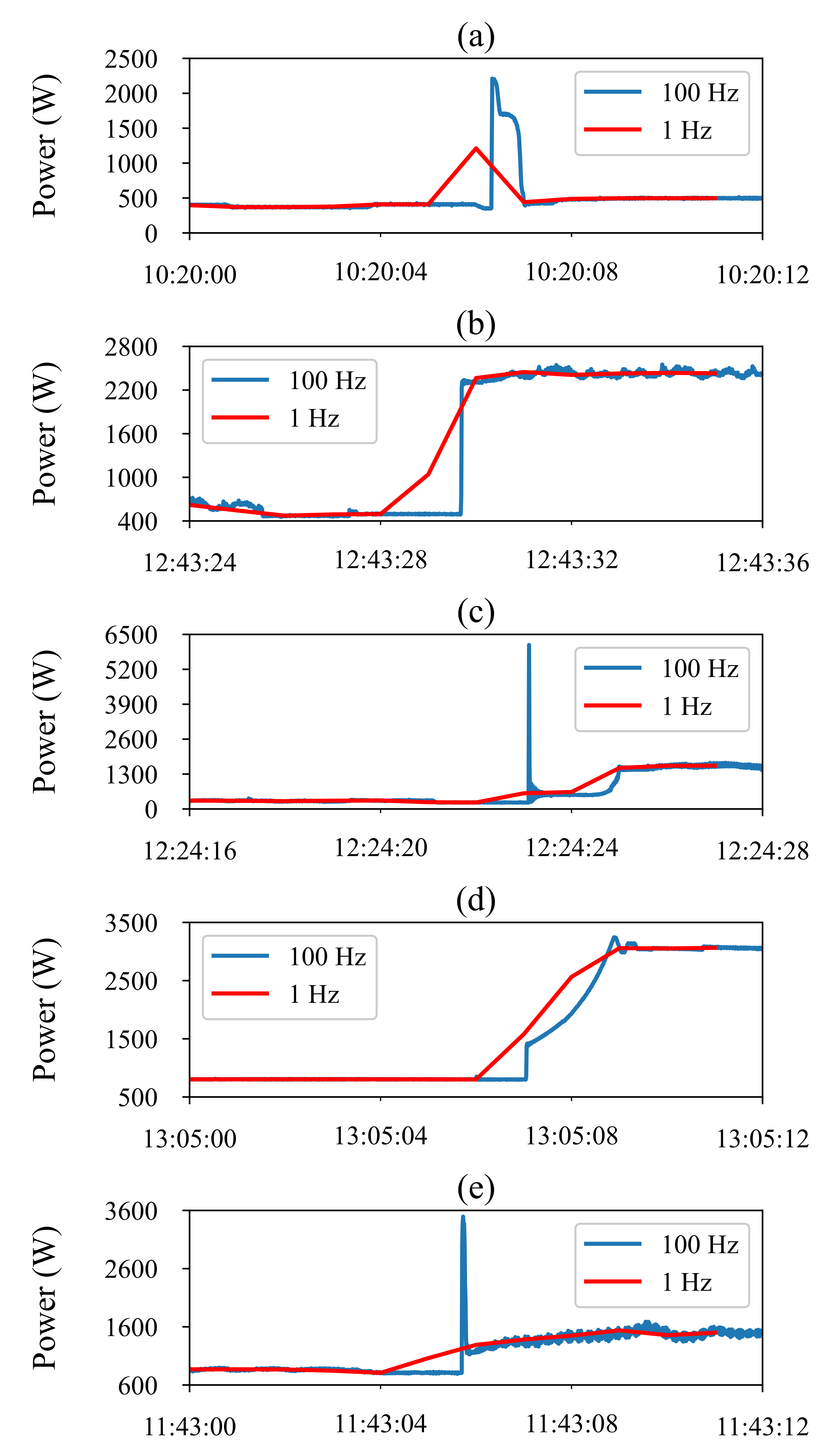
• Second comes the data resolution and as a result the data volumes required for an accurate NILM output. As mentioned above in Section 3, for real-time appliance identification sub-second data granularity is needed. Note that, most of the solutions presented in literature deal with kHz or even MHz of data. Considering as a rule of thumb that 1-s resolution data from separate phases in a 3-phase installation result in almost 1 GB of data being produced per year, we realize that moving into the kHz resolution areas makes data parsing, storing and analysing a rather complicated, costly and therefore non-scalable option.
• Next in the list comes the computational/RAM efficiency of such a service. Although the recent trend was to move everything to the cloud, now NILM vendors and energy companies realise that such a decision is not always the most cost-effective; the opposite actually. Running for example the whole service for ~100 k end users on the cloud can increase cloud operation costs that much, that there is no business case that can be built on top of a NILM layer, no matter how accurate that is. So, the key to unlock scalability opportunities here is to built a system that is so efficient that can run on the edge instead of the cloud.
• Strictly connected to the hardware constraints of the previous point comes the hardware cost. Traditionally sub-second data can be acquired only via a din meter hardware installed in the metering cabinet (it’s only recently that a few smart-meter manufacturers make >1 Hz resolutions available through their S1 port [53]). On the other hand, utilities and energy retail companies see NILM as a great customer engagement tool on top of which they can build value-added services and they usually tend to offer that as a freemium service. As a result, hardware cost has to be as low as possible and ideally within the companies customer retention and acquisition budgets.

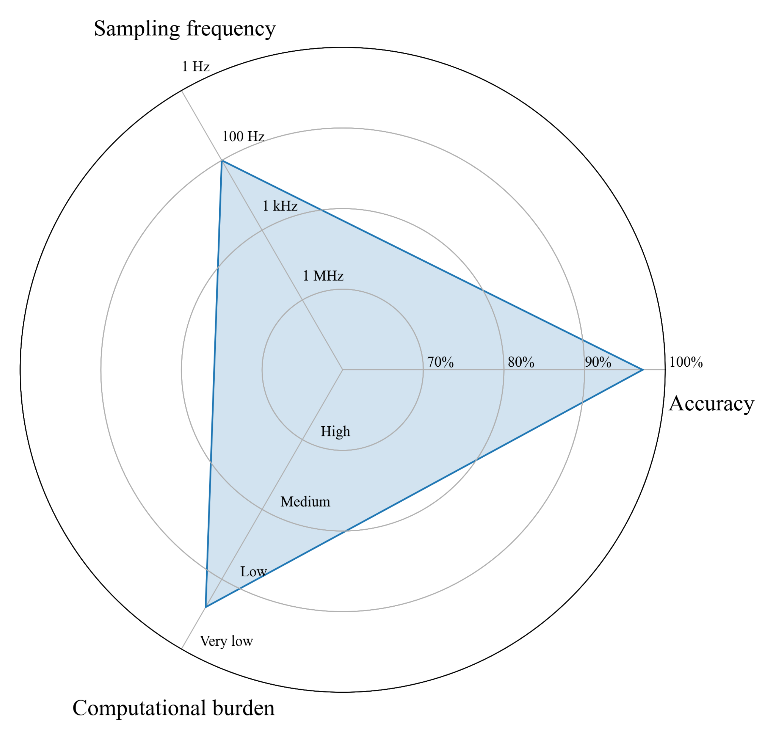
In Figure 7, three of the criteria mentioned above are analyzed for the proposed system, i.e., accuracy, sampling frequency, and computational burden. As we can see, scalability-related criteria #1 and #2 are met; the proposed system presents accuracy higher than 90% in all examined cases by utilizing the sampling frequency of 100 Hz (see results in Section 4). Although this frequency is high, it is still considerably lower than a resolution of several kHz used in most state-of-the-art real-time implementations [33,34,35,39]. To that end, it is an excellent “do a lot with a little” decision to take. Regarding criterion #3, i.e., computational and memory efficiency, as demonstrated in Section 4.5, optimized design can efficiently run on the edge and even on low-cost chip-sets. Specifically, in Figure 7, it is assumed that the “High” value refers to expensive algorithms, incorporating several parameters that cannot be easily integrated into a low-cost microprocessor. On the other hand, the “Very Low” value refers to low computational complexity algorithms that can be integrated and run in a low-cost microprocessor. The proposed system is between the “Low” and “Very Low” area. Criterion #4 is expected to be met as a consequence of #3. However, such an investigation falls out of the scope of this paper.

6. Conclusions

In this paper, a novel real-time event-based energy disaggregation methodology is introduced. Initially, a simple event-detection algorithm is proposed to find time instants when an appliance is turned-on and extract transient responses at 100 Hz. Next, a convolutional neural network classifier identifies if a transient response was caused by a target appliance. Finally, a power estimation algorithm is implemented considering appliance end-uses as pulses of constant power. Experimental results show a promising performance for specific appliances.

Unlike most relevant papers in the literature, the proposed non-intrusive load monitoring system can identify in real-time when an appliance is turned-on based on its information-rich transient response sampled at 100 Hz. Furthermore, it is delay-free since, once a target appliance has been turned-on, the active power can be directly calculated. Moreover, the system is computational and memory-efficient and can be integrated into smart meters.

The proposed approach can be used for a significant number of appliances with negligible error. However, energy consumption of specific appliances, e.g., heat pump, tumble dryer, including many states of operation, cannot be calculated by the proposed methodology. For such cases, dedicated algorithms should be implemented. As future steps, a more robust power estimation algorithm will be examined for multi-state appliance uses. Additionally, the proposed methodology will be tested on more types of appliances.

References

1. Wang, Y.; Chen, Q.; Hong, T.; Kang, C. Review of Smart Meter Data Analytics: Applications, Methodologies, and Challenges. IEEE Trans. Smart Grid 2019, 10, 3125–3148. [Google Scholar] [CrossRef] [Green Version]
2. Hayes, B.P.; Prodanovic, M. State Forecasting and Operational Planning for Distribution Network Energy Management Systems. IEEE Trans. Smart Grid 2016, 7, 1002–1011. [Google Scholar] [CrossRef]
3. Huang, Y.; Wang, L.; Guo, W.; Kang, Q.; Wu, Q. Chance Constrained Optimization in a Home Energy Management System. IEEE Trans. Smart Grid 2018, 9, 252–260. [Google Scholar] [CrossRef]
4. Buzau, M.M.; Tejedor-Aguilera, J.; Cruz-Romero, P.; Gómez-Expósito, A. Detection of Non-Technical Losses Using Smart Meter Data and Supervised Learning. IEEE Trans. Smart Grid 2019, 10, 2661–2670. [Google Scholar] [CrossRef]
5. Chakraborty, S.; Das, S. Application of Smart Meters in High Impedance Fault Detection on Distribution Systems. IEEE Trans. Smart Grid 2019, 10, 3465–3473. [Google Scholar] [CrossRef]
6. Chatzigeorgiou, I.; Andreou, G. A systematic review on feedback research for residential energy behavior change through mobile and web interfaces. Renew. Sust. Energ. Rev. 2021, 135, 110187. [Google Scholar] [CrossRef]
7. Nalmpantis, C.; Vrakas, D. Machine learning approaches for non-intrusive load monitoring: From qualitative to quantitative comparation. Artif. Intel. Rev. 2018, 52. [Google Scholar] [CrossRef]
8. Ruano, A.; Hernandez, A.; Ureña, J.; Ruano, M.; Garcia, J. NILM Techniques for Intelligent Home Energy Management and Ambient Assisted Living: A Review. Energies 2019, 12, 2203. [Google Scholar] [CrossRef] [Green Version]
9. Hart, G.W. Non-intrusive appliance load monitoring. Proc. IEEE 1992, 80, 1870–1891. [Google Scholar] [CrossRef]
10. Kolter, J.Z.; Jaakkola, T. Approximate Inference in Additive Factorial HMMs with Application to Energy Disaggregation. In Proceedings of the Fifteenth International Conference on Artificial Intelligence and Statistics, La Palma, Canary Islands, 21–23 April 2012; Volume 22, pp. 1472–1482. Available online: http://proceedings.mlr.press/v22/zico12.html (accessed on 15 January 2021).
11. Zoha, A.; Gluhak, A.; Nati, M.; Imran, M.A. Low-power appliance monitoring using Factorial Hidden Markov Models. In Proceedings of the 2013 IEEE Eighth International Conference on Intelligent Sensors, Sensor Networks and Information Processing, Melbourne, VIC, Australia, 2–5 April 2013; pp. 527–532. [Google Scholar] [CrossRef] [Green Version]
12. Bonfigli, R.; Principi, E.; Fagiani, M.; Severini, M.; Squartini, S.; Piazza, F. Non-intrusive load monitoring by using active and reactive power in additive Factorial Hidden Markov Models. Appl. Energy 2017, 208, 1590–1607. [Google Scholar] [CrossRef]
13. Lu, T.; Xu, Z.; Huang, B. An Event-Based Nonintrusive Load Monitoring Approach: Using the Simplified Viterbi Algorithm. IEEE Pervasive Comput. 2017, 16, 54–61. [Google Scholar] [CrossRef]
14. Ji, T.Y.; Liu, L.; Wang, T.S.; Lin, W.B.; Li, M.S.; Wu, Q.H. Non-Intrusive Load Monitoring Using Additive Factorial Approximate Maximum a Posteriori Based on Iterative Fuzzy c-Means. IEEE Trans. Smart Grid 2019, 10, 6667–6677. [Google Scholar] [CrossRef]
15. Makonin, S.; Popowich, F.; Bajic, I.V.; Gill, B.; Bartram, L. Exploiting HMM Sparsity to Perform Online Real-Time Nonintrusive Load Monitoring. IEEE Trans. Smart Grid 2016, 7, 2575–2585. [Google Scholar] [CrossRef]
16. Kong, W.; Dong, Z.Y.; Hill, D.J.; Ma, J.; Zhao, J.H.; Luo, F.J. A Hierarchical Hidden Markov Model Framework for Home Appliance Modeling. IEEE Trans. Smart Grid 2018, 9, 3079–3090. [Google Scholar] [CrossRef]
17. Mueller, J.A.; Kimball, J.W. Accurate Energy Use Estimation for Nonintrusive Load Monitoring in Systems of Known Devices. IEEE Trans. Smart Grid 2018, 9, 2797–2808. [Google Scholar] [CrossRef]
18. Kim, J.; Le, T.T.H.; Kim, H. Non-intrusive Load Monitoring Based on Advanced Deep Learning and Novel Signature. Comput. Intel. Neurosc. 2017, 2017, 4216281. [Google Scholar] [CrossRef]
19. Kelly, J.; Knottenbelt, W. Neural NILM. In Proceedings of the 2nd ACM International Conference on Embedded Systems for Energy-Efficient Built Environments—BuildSys’15, Seoul, Korea, 4–5 November 2015. [Google Scholar] [CrossRef] [Green Version]
20. Krystalakos, O.; Nalmpantis, C.; Vrakas, D. Sliding Window Approach for Online Energy Disaggregation Using Artificial Neural Networks. In Proceedings of the 10th Hellenic Conference on Artificial Intelligence, SETN ’18, Patra, Greece, 9–15 July 2018; Association for Computing Machinery: New York, NY, USA, 2018. [Google Scholar] [CrossRef]
21. Mauch, L.; Yang, B. A new approach for supervised power disaggregation by using a deep recurrent LSTM network. In Proceedings of the 2015 IEEE Global Conference on Signal and Information Processing (GlobalSIP), Orlando, FL, USA, 14–16 December 2015; pp. 63–67. [Google Scholar] [CrossRef]
22. Virtsionis Gkalinikis, N.; Nalmpantis, C.; Vrakas, D. Attention in Recurrent Neural Networks for Energy Disaggregation. In Discovery Science; Appice, A., Tsoumakas, G., Manolopoulos, Y., Matwin, S., Eds.; Springer International Publishing: Cham, Switzerland, 2020; pp. 551–565. [Google Scholar] [CrossRef]
23. Kaselimi, M.; Protopapadakis, E.; Voulodimos, A.; Doulamis, N.; Doulamis, A. Multi-Channel Recurrent Convolutional Neural Networks for Energy Disaggregation. IEEE Access 2019, 7, 81047–81056. [Google Scholar] [CrossRef]
24. Sudoso, A.M.; Piccialli, V. Non-Intrusive Load Monitoring with an Attention-based Deep Neural Network. arXiv 2019, arXiv:1912.00759. [Google Scholar]
25. He, W.; Chai, Y. An Empirical Study on Energy Disaggregation via Deep Learning. In Proceedings of the 2016 2nd International Conference on Artificial Intelligence and Industrial Engineering (AIIE 2016), Beijing, China, 20–21 November 2016; Atlantis Press: Amsterdam, The Netherlands, 2016; pp. 338–342. [Google Scholar] [CrossRef] [Green Version]
26. Zhang, C.; Zhong, M.; Wang, Z.; Goddard, N.; Sutton, C. Sequence-to-point learning with neural networks for non-intrusive load monitoring. arXiv 2016, arXiv:1612.09106. [Google Scholar]
27. Faustine, A.; Pereira, L.; Bousbiat, H.; Kulkarni, S. UNet-NILM: A Deep Neural Network for Multi-Tasks Appliances State Detection and Power Estimation in NILM. In Proceedings of the 5th International Workshop on Non-Intrusive Load Monitoring; NILM’20; Association for Computing Machinery: New York, NY, USA, 2020; pp. 84–88. [Google Scholar] [CrossRef]
28. Devlin, M.A.; Hayes, B.P. Non-Intrusive Load Monitoring and Classification of Activities of Daily Living Using Residential Smart Meter Data. IEEE Trans. Consum. Electron. 2019, 65, 339–348. [Google Scholar] [CrossRef]
29. Penha, D.; Castro, A. Home Appliance Identification for NILM Systems Based on Deep Neural Networks. Int. J. Artif. Intell. Appl. 2018, 9, 69–80. [Google Scholar] [CrossRef]
30. Kong, W.; Dong, Z.Y.; Wang, B.; Zhao, J.; Huang, J. A Practical Solution for Non-Intrusive Type II Load Monitoring Based on Deep Learning and Post-Processing. IEEE Trans. Smart Grid 2020, 11, 148–160. [Google Scholar] [CrossRef]
31. Cui, G.; Liu, B.; Luan, W.; Yu, Y. Estimation of Target Appliance Electricity Consumption Using Background Filtering. IEEE Trans. Smart Grid 2019, 10, 5920–5929. [Google Scholar] [CrossRef]
32. Alcalá, J.; Ureña, J.; Hernández, Á.; Gualda, D. Event-Based Energy Disaggregation Algorithm for Activity Monitoring From a Single-Point Sensor. IEEE Trans. Instrum. Meas. 2017, 66, 2615–2626. [Google Scholar] [CrossRef]
33. Faustine, A.; Pereira, L. Improved Appliance Classification in Non-Intrusive Load Monitoring Using Weighted Recurrence Graph and Convolutional Neural Networks. Energies 2020, 13, 3374. [Google Scholar] [CrossRef]
34. Yang, D.; Gao, X.; Kong, L.; Pang, Y.; Zhou, B. An Event-Driven Convolutional Neural Architecture for Non-Intrusive Load Monitoring of Residential Appliance. IEEE Trans. Consum. Electron. 2020, 66, 173–182. [Google Scholar] [CrossRef]
35. De Baets, L.; Ruyssinck, J.; Develder, C.; Dhaene, T.; Deschrijver, D. Appliance classification using VI trajectories and convolutional neural networks. Energ. Build. 2018, 158, 32–36. [Google Scholar] [CrossRef] [Green Version]
36. Liu, Y.; Wang, X.; You, W. Non-Intrusive Load Monitoring by Voltage—Current Trajectory Enabled Transfer Learning. IEEE Trans. Smart Grid 2019, 10, 5609–5619. [Google Scholar] [CrossRef]
37. Hassan, T.; Javed, F.; Arshad, N. An Empirical Investigation of V-I Trajectory Based Load Signatures for Non-Intrusive Load Monitoring. IEEE Trans. Smart Grid 2014, 5, 870–878. [Google Scholar] [CrossRef] [Green Version]
38. Du, L.; He, D.; Harley, R.G.; Habetler, T.G. Electric Load Classification by Binary Voltage—Current Trajectory Mapping. IEEE Trans. Smart Grid 2016, 7, 358–365. [Google Scholar] [CrossRef]
39. Faustine, A.; Pereira, L. Multi-Label Learning for Appliance Recognition in NILM Using Fryze-Current Decomposition and Convolutional Neural Network. Energies 2020, 13, 4154. [Google Scholar] [CrossRef]
40. Krizhevsky, A.; Sutskever, I.; Hinton, G. ImageNet Classification with Deep Convolutional Neural Networks. Neural Inf. Process Syst. 2012, 25. [Google Scholar] [CrossRef]
41. Chang, H.H.; Lin, L.S.; Chen, N.; Lee, W.J. Particle Swarm Optimization based non-intrusive demand monitoring and load identification in smart meters. In Proceedings of the 2012 IEEE Industry Applications Society Annual Meeting, Las Vegas, NV, USA, 7–11 October 2012; pp. 1–8. [Google Scholar] [CrossRef]
42. Chang, H.H.; Chen, K.L.; Tsai, Y.P.; Lee, W.J. A New Measurement Method for Power Signatures of Nonintrusive Demand Monitoring and Load Identification. IEEE Trans. Ind. Appl. 2012, 48, 764–771. [Google Scholar] [CrossRef]
43. Zoha, A.; Gluhak, A.; Imran, M.; Rajasegarar, S. Non-Intrusive Load Monitoring Approaches for Disaggregated Energy Sensing: A Survey. Sensors 2012, 12, 16838–16866. [Google Scholar] [CrossRef] [Green Version]
44. Revuelta Herrero, J.; Lozano Murciego, A.; Barriuso, A.; Hernández de la Iglesia, D.; Villarrubia, G.; Corchado Rodríguez, J.; Carreira, R. Non Intrusive Load Monitoring (NILM): A State of the Art. In Trends in Cyber-Physical Multi-Agent Systems; Springer International Publishing: Cham, Switzerland, 2018; pp. 125–138. [Google Scholar] [CrossRef]
45. LeCun, Y.; Bengio, Y.; Hinton, G. Deep Learning. Nature 2015, 521, 436–444. [Google Scholar] [CrossRef]
46. Srivastava, N.; Hinton, G.; Krizhevsky, A.; Sutskever, I.; Salakhutdinov, R. Dropout: A Simple Way to Prevent Neural Networks from Overfitting. J. Mach. Learn. Res. 2014, 15, 1929–1958. Available online: http://jmlr.org/papers/v15/srivastava14a.html (accessed on 15 January 2021).
47. Kingma, D.P.; Ba, J. Adam: A Method for Stochastic Optimization. arXiv 2017, arXiv:1412.6980. [Google Scholar]
48. Anderson, K.; Ocneanu, A.; Benitez, D.; Carlson, D.; Rowe, A.; Bergés, M. BLUED: A Fully Labeled Public Dataset for Event-Based Non-Intrusive Load Monitoring Research. In Proceedings of the 2nd KDD Workshop on Data Mining Applications in Sustainability (SustKDD), Beijing, China, 12 August 2012. [Google Scholar]
49. Lu, M.; Li, Z. A Hybrid Event Detection Approach for Non-Intrusive Load Monitoring. IEEE Trans. Smart Grid 2020, 11, 528–540. [Google Scholar] [CrossRef] [Green Version]
50. Bergés, M.; Goldman, E.; Matthews, H.; Soibelman, L.; Anderson, K. User-Centered Nonintrusive Electricity Load Monitoring for Residential Buildings. J. Comput. Civ. Eng. 2011, 25, 471–480. [Google Scholar] [CrossRef]
51. Kelly, J.; Knottenbelt, W. The UK-DALE dataset, domestic appliance-level electricity demand and whole-house demand from five UK homes. Sci. Data 2015, 2. [Google Scholar] [CrossRef] [Green Version]
52. Kolter, J.; Johnson, M. REDD: A Public Data Set for Energy Disaggregation Research. In Proceedings of the SustKDD Workshop on Data Mining Applications in Sustainability, San Diego, CA, USA, 21 August 2011. [Google Scholar]
53. Fluvius. User Ports of Smart Meters Explanatory Note on the Possibilities for Product Developers; Technical Report; Melle, Belgium, 2019; Available online: https://www.fluvius.be/sites/fluvius/files/2019-07/1901-fluvius-technical-specification-user-ports-digital-meter.pdf (accessed on 15 January 2021).
Figure 1. Proposed system flowchart.
Energies 14 00767 g001
Figure 2. Convolutional neural network (CNN) block diagram.
Energies 14 00767 g002
Figure 3. Comparison of the turn-on transient response with sampling frequency at 100 Hz and 1 Hz for (a) fridge, (b) washing machine, (c) microwave oven, (d) stove and (e) heat pump dryer.
Energies 14 00767 g003
Figure 4. Event detection in a real household on a given day.
Energies 14 00767 g004
Figure 5. Turn-on transient responses from different household appliances.
Energies 14 00767 g005
Figure 6. Power estimation for the selected appliances in real households. Time-series of (a) aggregated power, (b) actual target appliance power, (c) estimated power for fridge; (d) aggregated power, (e) actual target appliance power, (f) estimated power for washing machine; (g) aggregated power, (h) actual target appliance power, (i) estimated power for microwave.
Energies 14 00767 g006
Figure 7. Scalability evaluation of the proposed implementation.
Energies 14 00767 g007