Improving Non-Intrusive Load Disaggregation through an Attention-Based Deep Neural Network


Abstract
1. Introduction
2. NILM Problem
3. Encoder–Decoder with Attention Mechanism
3.1. Attention Mechanism
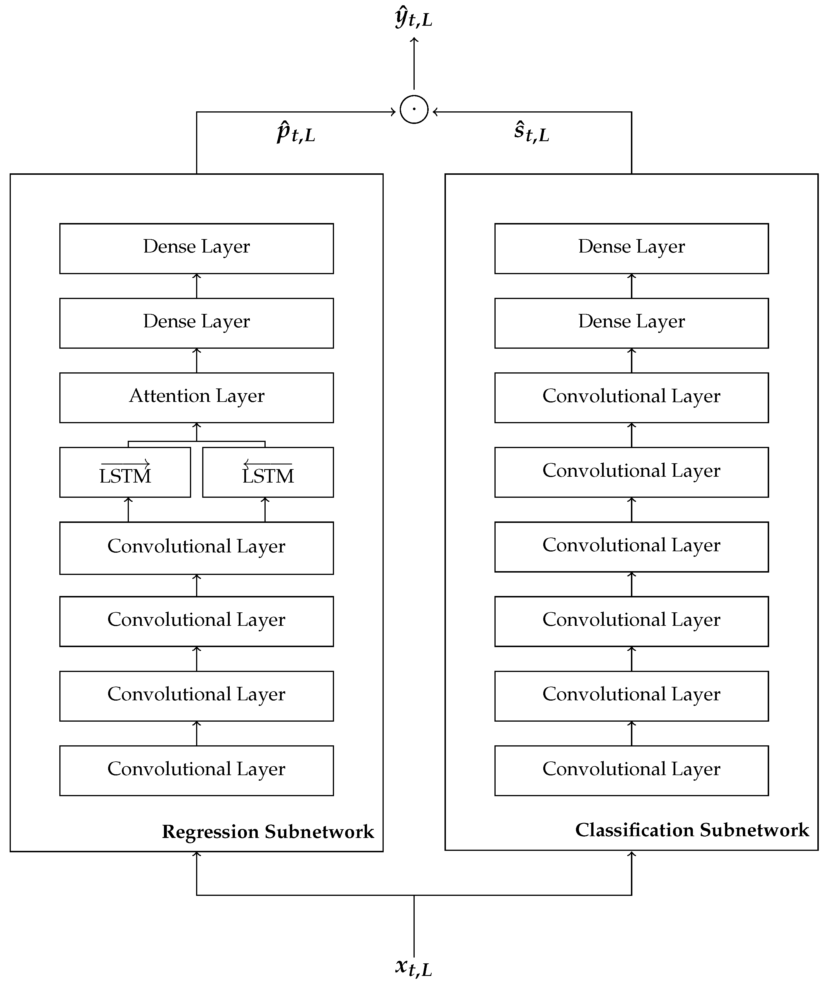
3.2. Model Design
3.3. Network Topology
- Input (sequence length L determined by the appliance duration)
- Conv1D (convolutional layer with F filters, kernel size K, stride 1, and ReLU activation function)
- Conv1D (convolutional layer with F filters, kernel size K, stride 1, and ReLU activation function)
- Conv1D (convolutional layer with F filters, kernel size K, stride 1, and ReLU activation function)
- Conv1D (convolutional layer with F filters, kernel size K, stride 1, and ReLU activation function)
- BiLSTM (bidirectional LSTM with H units, and tangent hyperbolic activation function)
- Attention (single layer feed-forward neural network with H units, and tangent hyperbolic activation function)
- Dense (fully connected layer with H units, and ReLU activation function)
- Dense (fully connected layer with L units, and linear activation function)
- Output (sequence length L)
- Input (sequence length L determined by the appliance duration)
- Conv1D (convolutional layer with 30 filters, kernel size 10, stride 1, and ReLU activation function)
- Conv1D (convolutional layer with 30 filters, kernel size 8, stride 1, and ReLU activation function)
- Conv1D (convolutional layer with 40 filters, kernel size 6, stride 1, and ReLU activation function)
- Conv1D (convolutional layer with 50 filters, kernel size 5, stride 1, and ReLU activation function)
- Conv1D (convolutional layer with 50 filters, kernel size 5, stride 1, and ReLU activation function)
- Conv1D (convolutional layer with 50 filters, kernel size 5, stride 1, and ReLU activation function)
- Dense (fully connected layer with 1024 units, and ReLU activation function)
- Dense (fully connected layer with L units, and sigmoid activation function)
- Output (sequence length L)
4. Experiments
4.1. Datasets
4.2. Metrics
4.3. Network Setup
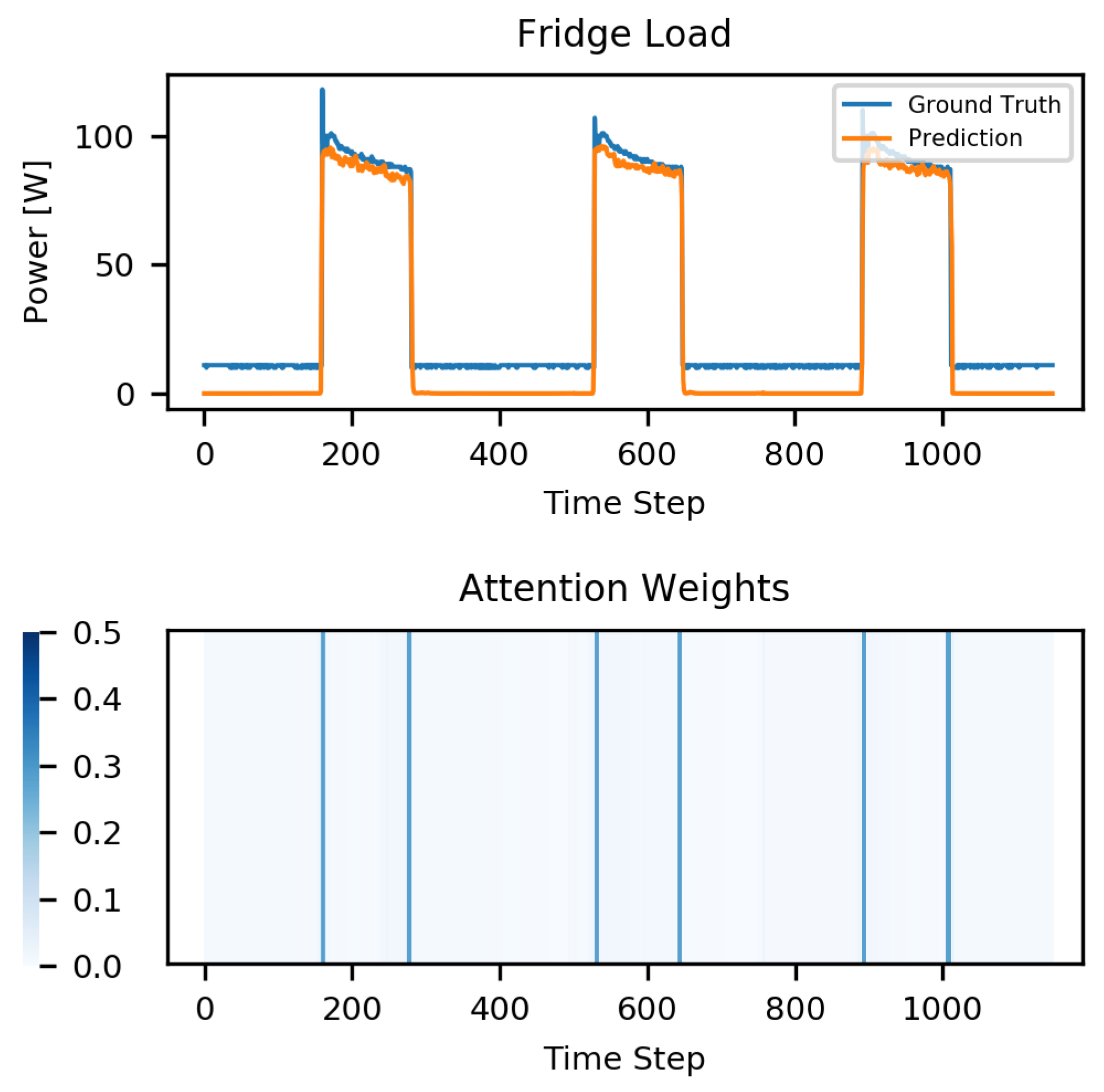
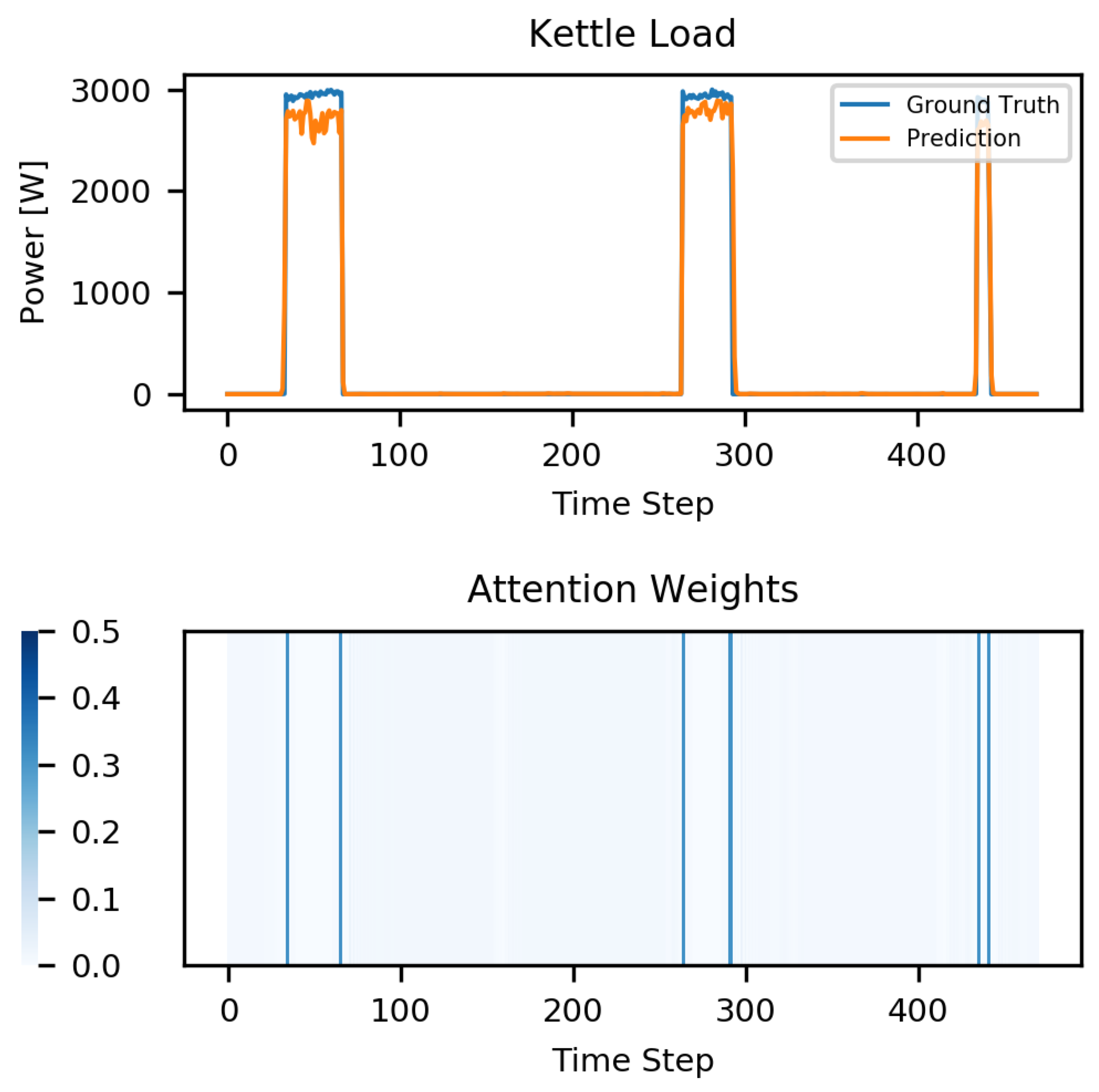
4.4. Results
5. Conclusions
Author Contributions
Funding
Institutional Review Board Statement
Informed Consent Statement
Data Availability Statement
Conflicts of Interest
References
- Hart, G.W. Nonintrusive appliance load monitoring. Proc. IEEE 1992, 80, 1870–1891. [Google Scholar] [CrossRef]
- Ruano, A.; Hernandez, A.; Ureña, J.; Ruano, M.; Garcia, J. NILM techniques for intelligent home energy management and ambient assisted living: A review. Energies 2019, 12, 2203. [Google Scholar] [CrossRef]
- de Souza, W.A.; Garcia, F.D.; Marafão, F.P.; Da Silva, L.C.P.; Simões, M.G. Load disaggregation using microscopic power features and pattern recognition. Energies 2019, 12, 2641. [Google Scholar] [CrossRef]
- Faustine, A.; Mvungi, N.H.; Kaijage, S.; Michael, K. A survey on non-intrusive load monitoring methodies and techniques for energy disaggregation problem. arXiv 2017, arXiv:1703.00785. [Google Scholar]
- Rahimpour, A.; Qi, H.; Fugate, D.; Kuruganti, T. Non-Intrusive Energy Disaggregation Using Non-Negative Matrix Factorization With Sum-to-k Constraint. IEEE Trans. Power Syst. 2017, 32, 4430–4441. [Google Scholar] [CrossRef]
- Kolter, J.Z.; Jaakkola, T. Approximate inference in additive factorial hmms with application to energy disaggregation. In Proceedings of the Fifteenth International Conference on Artificial Intelligence and Statistics, La Palma, Spain, 21–23 April 2012; pp. 1472–1482. [Google Scholar]
- Makonin, S.; Popowich, F.; Bajić, I.V.; Gill, B.; Bartram, L. Exploiting HMM sparsity to perform online real-time nonintrusive load monitoring. IEEE Trans. Smart Grid 2015, 7, 2575–2585. [Google Scholar] [CrossRef]
- Nashrullah, E.; Halim, A. Performance Evaluation of Superstate HMM with Median Filter For Appliance Energy Disaggregation. In Proceedings of the 2019 6th International Conference on Electrical Engineering, Computer Science and Informatics (EECSI), Bandung, Indonesia, 18–20 September 2019; pp. 374–379. [Google Scholar]
- Basu, K.; Debusschere, V.; Bacha, S.; Maulik, U.; Bondyopadhyay, S. Nonintrusive load monitoring: A temporal multilabel classification approach. IEEE Trans. Ind. Inform. 2014, 11, 262–270. [Google Scholar] [CrossRef]
- Singhal, V.; Maggu, J.; Majumdar, A. Simultaneous detection of multiple appliances from smart-meter measurements via multi-label consistent deep dictionary learning and deep transform learning. IEEE Trans. Smart Grid 2018, 10, 2969–2978. [Google Scholar] [CrossRef]
- Singh, S.; Majumdar, A. Non-Intrusive Load Monitoring via Multi-Label Sparse Representation-Based Classification. IEEE Trans. Smart Grid 2019, 11, 1799–1801. [Google Scholar] [CrossRef]
- Faustine, A.; Pereira, L. Multi-Label Learning for Appliance Recognition in NILM Using Fryze-Current Decomposition and Convolutional Neural Network. Energies 2020, 13, 4154. [Google Scholar] [CrossRef]
- Kelly, J.; Knottenbelt, W. Neural nilm: Deep neural networks applied to energy disaggregation. In Proceedings of the 2nd ACM International Conference on Embedded Systems for Energy-Efficient Built Environments, Seoul, Korea, 4–5 November 2015; pp. 55–64. [Google Scholar]
- He, W.; Chai, Y. An Empirical Study on Energy Disaggregation via Deep Learning. In Proceedings of the 2016 2nd International Conference on Artificial Intelligence and Industrial Engineering (AIIE 2016), Beijing, China, 20–21 November 2016. [Google Scholar]
- Zhang, C.; Zhong, M.; Wang, Z.; Goddard, N.; Sutton, C. Sequence-to-point learning with neural networks for non-intrusive load monitoring. In Proceedings of the Thirty-Second AAAI Conference on Artificial Intelligence, New Orleans, LA, USA, 2–7 February 2018. [Google Scholar]
- Bonfigli, R.; Felicetti, A.; Principi, E.; Fagiani, M.; Squartini, S.; Piazza, F. Denoising autoencoders for non-intrusive load monitoring: Improvements and comparative evaluation. Energy Build. 2018, 158, 1461–1474. [Google Scholar] [CrossRef]
- Shin, C.; Joo, S.; Yim, J.; Lee, H.; Moon, T.; Rhee, W. Subtask gated networks for non-intrusive load monitoring. In Proceedings of the AAAI Conference on Artificial Intelligence, Honolulu, HI, USA, 27 January–1 February 2019; Volume 33, pp. 1150–1157. [Google Scholar]
- Chen, K.; Zhang, Y.; Wang, Q.; Hu, J.; Fan, H.; He, J. Scale-and Context-Aware Convolutional Non-intrusive Load Monitoring. IEEE Trans. Power Syst. 2019, 35, 2362–2373. [Google Scholar] [CrossRef]
- Kong, W.; Dong, Z.Y.; Wang, B.; Zhao, J.; Huang, J. A Practical Solution for Non-Intrusive Type II Load Monitoring Based on Deep Learning and Post-Processing. IEEE Trans. Smart Grid 2020, 11, 148–160. [Google Scholar] [CrossRef]
- Wang, K.; Zhong, H.; Yu, N.; Xia, Q. Nonintrusive Load Monitoring based on Sequence-to-sequence Model With Attention Mechanism. Zhongguo Dianji Gongcheng Xuebao/Proc. Chin. Soc. Electr. Eng. 2019, 39, 75–83. [Google Scholar] [CrossRef]
- Bahdanau, D.; Cho, K.; Bengio, Y. Neural machine translation by jointly learning to align and translate. arXiv 2014, arXiv:1409.0473. [Google Scholar]
- Sutskever, I.; Vinyals, O.; Le, Q.V. Sequence to sequence learning with neural networks. In Advances in Neural Information Processing Systems 27, Proceedings of the 27th International Conference on Neural Information Processing Systems, December 2014, Pages 3104–3112; Montreal, Canada 2014; Ghahramani, Z., Welling, M., Cortes, C., Lawrence, N., Weinberger, K.Q., Eds.; MIT Press: Cambridge, MA, USA, 2014; pp. 3104–3112. [Google Scholar]
- Cho, K.; Van Merriënboer, B.; Bahdanau, D.; Bengio, Y. On the properties of neural machine translation: Encoder-decoder approaches. arXiv 2014, arXiv:1409.1259. [Google Scholar]
- Young, T.; Hazarika, D.; Poria, S.; Cambria, E. Recent trends in deep learning based natural language processing. IEEE Comput. Intell. Mag. 2018, 13, 55–75. [Google Scholar] [CrossRef]
- Raffel, C.; Ellis, D.P. Feed-forward networks with attention can solve some long-term memory problems. arXiv 2015, arXiv:1512.08756. [Google Scholar]
- Kolter, J.Z.; Johnson, M.J. REDD: A public data set for energy disaggregation research. In Proceedings of the Workshop on Data Mining Applications in Sustainability (SIGKDD), San Diego, CA, USA, 21–24 August 2011; Volume 25, pp. 59–62. [Google Scholar]
- Kelly, J.; Knottenbelt, W. The UK-DALE dataset, domestic appliance-level electricity demand and whole-house demand from five UK homes. Sci. Data 2015, 2, 150007. [Google Scholar] [CrossRef] [PubMed]
- Sutskever, I.; Martens, J.; Dahl, G.; Hinton, G. On the importance of initialization and momentum in deep learning. In Proceedings of the International Conference on Machine Learning, Atlanta, GA, USA, 16–21 June 2013; pp. 1139–1147. [Google Scholar]
- Caruana, R.; Lawrence, S.; Giles, L. Overfitting in Neural Nets: Backpropagation, Conjugate Gradient, and Early Stopping. In Proceedings of the 13th International Conference on Neural Information Processing Systems; MIT Press: Cambridge, MA, USA, 2000; pp. 381–387. [Google Scholar]
- Paszke, A.; Gross, S.; Chintala, S.; Chanan, G.; Yang, E.; DeVito, Z.; Lin, Z.; Desmaison, A.; Antiga, L.; Lerer, A. Automatic Differentiation in PyTorch. In Proceedings of the NIPS Autodiff Workshop, Long Beach, CA, USA, 9 December 2017. [Google Scholar]
- Batra, N.; Kelly, J.; Parson, O.; Dutta, H.; Knottenbelt, W.; Rogers, A.; Singh, A.; Srivastava, M. NILMTK: An open source toolkit for non-intrusive load monitoring. In Proceedings of the 5th International Conference on Future Energy Systems, Cambridge, UK, 11–13 June 2014; pp. 265–276. [Google Scholar]


| Dataset | DW | FR | KE | MW | WM |
|---|---|---|---|---|---|
| REDD | 2304 | 496 | - | 128 | - |
| UK-DALE | 1536 | 512 | 128 | 288 | 1024 |
| Model | Metric | DW | FR | MW | Overall |
|---|---|---|---|---|---|
| FHMM [31] | MAE | 101.30 | 98.67 | 87.00 | 95.66 |
| SAE | 93.64 | 46.73 | 65.03 | 68.47 | |
| F1 (%) | 12.93 | 35.12 | 11.97 | 20.01 | |
| DAE [16] | MAE | 26.18 | 29.11 | 23.26 | 26.18 |
| SAE | 21.46 | 20.97 | 19.14 | 20.52 | |
| F1 (%) | 48.81 | 74.76 | 18.54 | 47.37 | |
| Seq2Point [15] | MAE | 24.44 | 26.01 | 27.13 | 25.86 |
| SAE | 22.87 | 16.24 | 18.89 | 19.33 | |
| F1 (%) | 47.66 | 75.12 | 17.43 | 46.74 | |
| S2SwA [20] | MAE | 23.48 | 25.98 | 24.27 | 24.57 |
| SAE | 22.64 | 17.26 | 16.19 | 18.69 | |
| F1 (%) | 49.32 | 76.98 | 19.31 | 48.57 | |
| SGN [17] | MAE | 15.77 | 26.11 | 16.95 | 19.61 |
| SAE | 15.22 | 17.28 | 12.49 | 15.00 | |
| F1 (%) | 58.78 | 80.09 | 44.98 | 61.28 | |
| SCANet [18] | MAE | 10.14 | 21.77 | 13.75 | 15.22 |
| SAE | 8.12 | 14.05 | 9.97 | 10.71 | |
| F1 (%) | 69.21 | 83.12 | 57.43 | 69.92 | |
| Proposed LDwA | MAE | 8.65 | 19.81 | 11.17 | 13.21 |
| SAE | 6.94 | 13.23 | 7.12 | 9.10 | |
| F1 (%) | 74.41 | 86.76 | 69.01 | 76.73 |
| Model | Metric | DW | FR | KE | MW | WM | Overall |
|---|---|---|---|---|---|---|---|
| FHMM [31] | MAE | 48.25 | 60.93 | 38.02 | 43.63 | 67.91 | 51.75 |
| SAE | 46.04 | 51.90 | 35.41 | 41.52 | 64.15 | 47.80 | |
| F1 (%) | 11.79 | 33.52 | 9.35 | 3.44 | 4.10 | 12.44 | |
| DAE [16] | MAE | 22.18 | 17.72 | 10.87 | 12.87 | 13.64 | 15.46 |
| SAE | 18.24 | 8.74 | 7.95 | 9.99 | 10.67 | 11.12 | |
| F1 (%) | 54.88 | 75.98 | 93.43 | 31.32 | 24.54 | 56.03 | |
| Seq2Point [15] | MAE | 15.96 | 17.48 | 10.81 | 12.47 | 10.87 | 13.52 |
| SAE | 10.65 | 8.01 | 5.30 | 10.33 | 8.69 | 8.60 | |
| F1 (%) | 50.92 | 80.32 | 94.88 | 45.41 | 49.11 | 64.13 | |
| S2SwA [20] | MAE | 14.96 | 16.47 | 12.02 | 10.37 | 9.87 | 12.74 |
| SAE | 10.68 | 7.81 | 5.78 | 8.33 | 8.09 | 8.14 | |
| F1 (%) | 53.67 | 79.04 | 94.62 | 47.99 | 45.79 | 64.22 | |
| SGN [17] | MAE | 10.91 | 16.27 | 8.09 | 5.62 | 9.74 | 10.13 |
| SAE | 7.86 | 6.61 | 5.03 | 4.32 | 7.14 | 6.20 | |
| F1 (%) | 60.02 | 84.43 | 96.32 | 58.55 | 61.12 | 72.09 | |
| SCANet [18] | MAE | 8.71 | 15.16 | 6.14 | 4.82 | 8.48 | 8.67 |
| SAE | 4.86 | 6.54 | 4.03 | 3.81 | 5.77 | 5.00 | |
| F1 (%) | 63.30 | 85.77 | 98.89 | 62.22 | 63.09 | 74.65 | |
| Proposed LDwA | MAE | 6.57 | 13.24 | 5.69 | 3.79 | 7.26 | 7.31 |
| SAE | 3.91 | 6.02 | 3.74 | 2.98 | 4.87 | 4.30 | |
| F1 (%) | 68.99 | 87.01 | 99.81 | 67.55 | 71.94 | 79.06 |
Publisher’s Note: MDPI stays neutral with regard to jurisdictional claims in published maps and institutional affiliations. |
© 2021 by the authors. Licensee MDPI, Basel, Switzerland. This article is an open access article distributed under the terms and conditions of the Creative Commons Attribution (CC BY) license (http://creativecommons.org/licenses/by/4.0/).
Share and Cite
Piccialli, V.; Sudoso, A.M. Improving Non-Intrusive Load Disaggregation through an Attention-Based Deep Neural Network. Energies 2021, 14, 847. https://doi.org/10.3390/en14040847
Piccialli V, Sudoso AM. Improving Non-Intrusive Load Disaggregation through an Attention-Based Deep Neural Network. Energies. 2021; 14(4):847. https://doi.org/10.3390/en14040847
Chicago/Turabian StylePiccialli, Veronica, and Antonio M. Sudoso. 2021. "Improving Non-Intrusive Load Disaggregation through an Attention-Based Deep Neural Network" Energies 14, no. 4: 847. https://doi.org/10.3390/en14040847
APA StylePiccialli, V., & Sudoso, A. M. (2021). Improving Non-Intrusive Load Disaggregation through an Attention-Based Deep Neural Network. Energies, 14(4), 847. https://doi.org/10.3390/en14040847