Huber-Based Robust Unscented Kalman Filter Distributed Drive Electric Vehicle State Observation

Abstract

Accurate and real-time acquisition of vehicle state parameters is key to improving the performance of vehicle control systems. To improve the accuracy of state parameter estimation for distributed drive electric vehicles, an unscented Kalman filter (UKF) algorithm combined with the Huber method is proposed. In this paper, we introduce the nonlinear modified Dugoff tire model, build a nonlinear three-degrees-of-freedom time-varying parametric vehicle dynamics model, and extend the vehicle mass, the height of the center of gravity, and the yaw moment of inertia, which are significantly influenced by the driving state, into the vehicle state vector. The vehicle state parameter observer was designed using an unscented Kalman filter framework. The Huber cost function was introduced to correct the measured noise and state covariance in real-time to improve the robustness of the observer. The simulation verification of a double-lane change and straight-line driving conditions at constant speed was carried out using the Simulink/Carsim platform. The results show that observation using the Huber-based robust unscented Kalman filter (HRUKF) more realistically reflects the vehicle state in real-time, effectively suppresses the influence of abnormal error and noise, and obtains high observation accuracy.

1. Introduction

Due to the development of vehicle intelligence in recent years, an increasing number of active safety control systems have been widely used in vehicles, including electronic body stability systems, electronic brake-force distribution systems, drive anti-skid systems, and active steering systems. However, a stable and reliable control system does not only lie in the robustness of the control algorithm, but also relies on the accurate acquisition of key vehicle dynamic state parameters. Unlike conventional vehicles, distributed-drive electric vehicles are driven independently by four motors, and changes in the vehicle mass, the yaw moment of inertia, and the height of the center of gravity directly affect the vehicle driving state; for example, changes in the vehicle mass directly affect the vehicle’s economy and handling stability, and a change in the height of the center of mass has a significant impact on the vehicle’s roll stability. The amount of lateral load transfer is also affected by changes in the vehicle mass and the height of the center of gravity, thus affecting the vehicle driving state vector, and the MAP characteristics of the vehicle drive motor efficiency are related to the motor speed and torque. Therefore, for the characteristics of distributed drive electric vehicles, more accurate state parameters must be obtained, and the estimation and identification of these state parameters are particularly important. Estimation of vehicle condition parameters is necessary, because many condition parameters are not directly measured or obtained by sensors due to sensor price limitations and current technology constraints. At present, the widely studied estimates mainly include the vehicle sideslip angle, yaw rate, longitudinal velocity, tire force, and peak road adhesion coefficient, which do not involve the identification of the vehicle parameters [1,2,3]. The accurate identification of vehicle parameters is an important part in the design process of the vehicle active safety control system, and its accuracy and robustness directly affect the effectiveness of the controller. The change in these parameters affects the convergence of the controller. If the controller diverges when the vehicle is running at high speed, it can lead to serious traffic safety accidents. Thus, the acquisition of the vehicle’s own parameters and the improvement of the robustness of the controller are particularly important. Huang et al. proposed an adaptive unscented Kalman filter (UKF) to estimate the vehicle state, including state vectors such as velocity, yaw rate, and vehicle sideslip angle [4]. Wielitzka et al. designed a joint observer of an unscented Kalman filter to estimate the vehicle mass, vehicle sideslip angle, and yaw moment of inertia, which effectively improved the estimation accuracy of vehicle state parameters [5]. Jiang et al. combined recursive least squares algorithm (RLS) and KF algorithms to estimate vehicle parameters and states, respectively, using RLS for vehicle mass, road slope, the height of the center of gravity, and suspension stiffness, and a dual extended Kalman filter (EKF) for vehicle load transfer and tire vertical force, effectively improving the robustness of the observer [6]. Hong et al. estimated the center-of-mass position, the vehicle mass, and the yaw moment of inertia based on a double Kalman filter, but did not consider the effect of the height of the center of gravity [7]. BOADA et al. performed parameter identification based on a double Kalman filter for road slope, tire lateral deflection stiffness, suspension stiffness, and the height of the center of gravity [8]. The above-mentioned paper uses a variety of methods to identify the vehicle state parameters, but it is difficult to achieve effective estimation for systems with strong nonlinearity using these methods, and the vehicle state vectors considered for parameter estimation are small. The vehicle’s own parameters, including mass, yaw moment of inertia, and the height of the center of gravity, directly affect the lateral tire forces, which in turn affect the vehicle’s lateral and longitudinal velocity, acceleration, sideslip angle, yaw rate, and other state vectors.

The Kalman filter has successfully been applied in many fields as an optimal minimum norm estimation. However, the standard Kalman filter is only applicable to linear systems, and the vehicle system, as a strong nonlinear system, cannot be directly applied to the standard Kalman filter framework. One method is to linearize the nonlinear system, such as the extended Kalman filter (EKF); however, the EKF method can only achieve first-order Taylor accuracy and requires solving the Jacobian matrix, which can be difficult when the model is complex. Another method uses statistical linearization to approximate nonlinear equations, such as the unscented transform (UT) method used by the unscented Kalman filter, which approximates the probability density distribution for nonlinear functions without solving the complex Jacobian matrix. In addition, the estimation accuracy can reach the second-order accuracy of the Taylor series expansion [9,10], with advantages of high computational accuracy and good stability. Thus, the UKF algorithm is chosen as the basis of vehicle state parameter estimation in this paper [9,10].

In 1964, Huber proposed a method based on minimizing the error of the paradigm, the Huber method, to improve the robustness of the algorithm under the noise of the perturbing Gaussian distribution, by minimizing the error asymptotically. This approach is more robust than the paradigm-based estimation method [11]. L. Chang et al. introduced the Huber method into the UKF framework to study the UKF algorithm under a non-Gaussian probability distribution and used the Huber cost function to modify the standard UKF measurement update equation. Numerical simulations proved the effectiveness of the algorithm [12]. Jing Hou et al. designed a Huber-based robust cubature Kalman filter (CKF) observer for state of charge (SOC) state observation of batteries, which enhances the robustness to values of current and voltage measurements caused by abnormal operation [13]. Lu Xiong et al. designed an algorithm for the autonomous underwater vehicle (AUV) terrain matching problem based on the Huber method in combination with UKF, and the results show that the substitution of the Huber method into the UKF framework can effectively improve the robustness of the algorithm [14]. Currently, the Huber method is often used in the CKF framework and is widely used in battery SOC, power grid system state estimation, combined INS/DVL navigation, and target tracking. However, it has not yet been used in distributed drive electric vehicle (EV) state parameter estimation [15,16,17,18]. In this study, the Huber method is introduced into the UKF vehicle state parameter estimation framework to correct for the measured noise and state covariance in real-time, which reduces the convergence time and improves the robustness and estimation accuracy of the algorithm. This study used distributed drive electric vehicles as the research object. The main stages were to consider the variation caused by the interaction of vehicle mass, height of the center of gravity, and yaw moment of inertia; expand the above vehicle parameters into the vehicle state vector; design an observer that can simultaneously estimate the vehicle state and parameters; and introduce the Huber method into the UKF vehicle state parameter estimation framework to correct the measurement noise and state covariance in real-time. The result was to reduce the convergence time and improve the robustness and estimation accuracy of the algorithm.

2. Nonlinear Time-Varying Parametric Vehicle Dynamics Model

2.1. Vehicle Model

The parameters of the vehicle during the driving process, including the height of the center of mass and the moment of inertia, are affected by the driving state of the vehicle and the vehicle load. The change of the height of the center of gravity of the vehicle is particularly important for the vehicle’s stability control. The vehicle dynamics model studied in this paper is shown in Figure 1. The origin of the defined vehicle coordinate system is located at the center of gravity (CG), and the forward direction of the vehicle is defined as the positive axis direction; the left side is the positive direction of the y-axis, and the positive direction of the z-axis is perpendicular to the ground. It is assumed that the pitch, vertical, and roll motions of the vehicle are ignored, and the influence of the suspension system is ignored. Furthermore, the influence of the camber angle and the return torque of the wheels on the dynamics of the vehicle is ignored. This is the state parameter required for vehicle stability control. We established a three-degrees-of-freedom dynamic model of a distributed drive electric vehicle with nonlinear time-varying parameters including yaw, longitudinal, and lateral motion [19]. The vehicle dynamics equations are as follows.

The equation of the longitudinal motion is:

$$m(t)({\dot{V}}_x-V_y\dot{\psi })={\displaystyle \sum _{i,j=1}^2{F}_{xij}}=m(t)a_x$$

(1)

$${\displaystyle \sum _{i,j=1}^2{F}_{xij}}=F_{x11}\cos {\delta }_{11}+F_{x12}\cos {\delta }_{12}-F_{y11}\sin {\delta }_{11}-F_{y12}\sin {\delta }_{12}+F_{x21}+F_{x22}$$

(2)

The equation of the lateral motion is:

$$m(t)({\dot{V}}_y-V_x\dot{\psi })={\displaystyle \sum _{i,j=1}^2{F}_{yij}}=m(t)a_y$$

(3)

$${\displaystyle \sum _{i,j=1}^2{F}_{yij}}=F_{x11}\sin {\delta }_{11}+F_{x12}\sin {\delta }_{12}+F_{y11}\cos {\delta }_{11}+F_{y12}\cos {\delta }_{12}+F_{y21}+F_{y22}$$

(4)

The equation of the yaw motion is:

$$I_{zz}(t)\ddot{\psi }={\displaystyle \sum _{i,j=1}^2{M}_z{}_{ij}}$$

(5)

$$\begin{array}{r}{\displaystyle \sum _{i,j=1}^2{M}_z{}_{ij}}=a(F_{y11}\cos {\delta }_{11}+F_{y12}\cos {\delta }_{12})+a(F_{x11}\sin {\delta }_{11}+F_{x12}\sin {\delta }_{12})-\\ \frac{w}{2}(F_{y11}\sin {\delta }_{11}-F_{y12}\sin {\delta }_{12})+\frac{w}{2}(F_{x11}\cos {\delta }_{11}-F_{x12}\cos {\delta }_{12})-\\ b(F_{y21}+F_{y22})+\frac{w}{2}(F_{x21}-F_{x22})\end{array}$$

(6)

where $V_x$, $V_y$ are the longitudinal and lateral velocities; $\dot{\psi }$ is the yaw rate of the vehicle; $a_x$ and $a_y$ are longitudinal acceleration and lateral acceleration, respectively; $F_{xij}$ and $F_{yij}$ are longitudinal and lateral forces of the four wheels, respectively, where $ij$ is 11, 12, 21, and 22, which represent the front left, front right, rear left, and rear right wheel, respectively. $M_z$ represents the yaw moment of the vehicle; m is the vehicle mass; w is the track width; a and b are the distances from the gravity center to the front and the rear axles, respectively; L is the wheelbase; $I_{zz}$ is the moment of inertia of the vehicle around the axis; and ${\delta }_{11}$ and ${\delta }_{12}$ are the steering angles of the left and right front wheels, respectively.

When the vehicle is turned, the longitudinal force and the lateral force of the tire are affected by the transfer of the vertical load by the following equation:

$$\begin{array}{c}{F}_{z1j}=\frac{b}{2L}m(t)g-\frac{h_g(t)}{2L}m(t)a_x\mp \frac{b{h}_g(t)}{Lw}m(t)a_y\\ F_{z2j}=\frac{a}{2L}m(t)g+\frac{h_g(t)}{2L}m(t)a_x\pm \frac{a{h}_g(t)}{Lw}m(t)a_y\end{array}\}$$

(7)

where $h_g$ is the height of the center of gravity, and $F_{z1j}$ and $F_{z2j}$ are the vertical load of the left front wheel and the right front wheel, respectively.

The sideslip angle of the tire is calculated as follows:

$$\begin{array}{c}{\alpha }_{1j}=\delta -\arctan (\frac{V_y+a\dot{\psi }}{V_x\mp w\dot{\psi }/2})\\ {\alpha }_{2j}=-\arctan (\frac{V_y-b\dot{\psi }}{V_x\pm w\dot{\psi }/2})\end{array}\}$$

(8)

where ${\alpha }_{1j}$ and ${\alpha }_{2j}$ are the sideslip angle of the front tire and the rear tires, respectively.

2.2. Tire Model

As a typical component of a ground vehicle, tires transfer the vehicle forces and torques to the road through the tire’s grounding area, and their performance directly affects the vehicle dynamic characteristics. In the current theoretical research, the Magic Formula tire model and the Dugoff tire model are mainly used. However, the Dugoff tire model was chosen in this study because the MF model requires a large number of tests to obtain the empirical parameters. The Dugoff tire model has no peak point, and the maximum value is smaller than the maximum value of the MF model. As the slip rate increases, the difference between the longitudinal forces of the Dugoff tire model and the MF model increases, and as the tire slip angle increases, the difference between the lateral forces of the two models also increases [20,21]. In view of the above points, the modified Dugoff tire model was used for modeling, and can be described by:

$$F_{xij}=C_{xij}\frac{\tan {\alpha }_{ij}}{1+{\lambda }_{ij}}f({\sigma }_{ij}){\varphi }_{xij}$$

(9)

$$F_{yij}=C_{yij}\frac{\tan {\alpha }_{ij}}{1+{\lambda }_{ij}}f({\sigma }_{ij}){\varphi }_{yij}$$

(10)

$${\sigma }_{ij}=\frac{{\mu }_{ij\max }{F}_{zij}(1+{\lambda }_{ij})}{2\sqrt{{(C_{xij}{\lambda }_{ij})}^2+{(C_{yij}\tan {\alpha }_{ij})}^2}}$$

(11)

$${\varphi }_{xij}=(1.15-0.75{\mu }_{ij\max }){\lambda }_{ij}^2-(1.63-0.75{\mu }_{ij\max }){\lambda }_{ij}+1.27$$

(12)

$${\varphi }_{yij}=(-1.6+{\mu }_{ij\max })\tan {\alpha }_{ij}+1.155$$

(13)

$$f({\sigma }_{ij})=\{\begin{array}{c}{\sigma }_{ij}(2-{\sigma }_{ij})\\ 1\end{array}\begin{array}{c}({\sigma }_{ij}\le 1)\\ ({\sigma }_{ij}>1)\end{array}$$

(14)

$${\lambda }_{ij}=\frac{R{\omega }_{ij}-V_x}{\max (R{\omega }_{ij},V_x)}$$

(15)

where $C_{xij}$ and $C_{yij}$ are the longitudinal and lateral stiffness of the four tires, respectively; ${\mu }_{ij\max }$ is the pavement peak adhesion coefficient; ${\varphi }_{xij}$ and ${\varphi }_{yij}$ are the longitudinal and lateral correction coefficients of the tires, respectively; and ${\lambda }_{ij}$ is the slip rate.

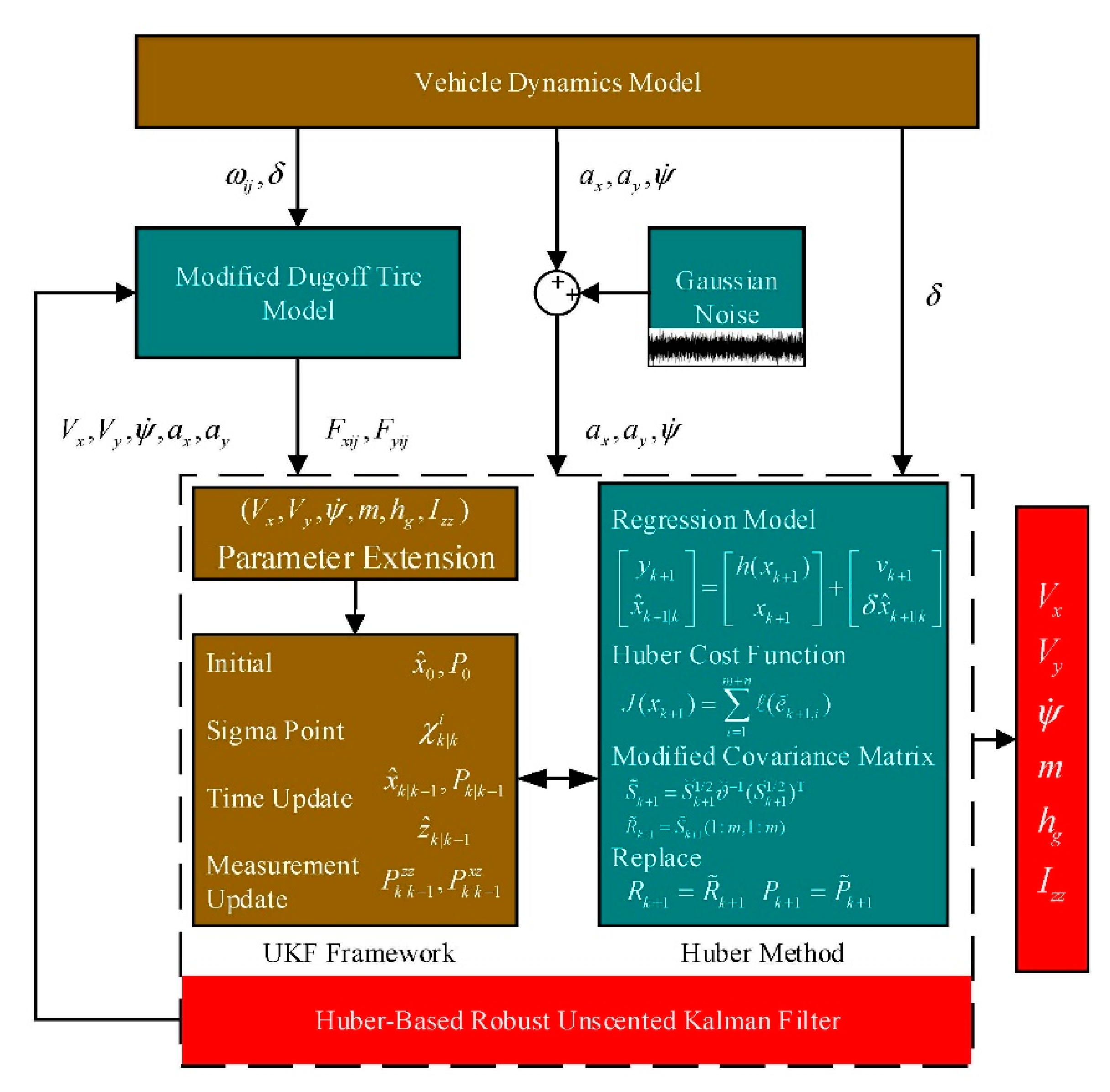
3. Huber-Based Robust Unscented Kalman Filter (HRUKF)

To design a Huber-based robust unscented Kalman filter state observer, the corresponding state and observation quantities were selected, the state and observation equations of the nonlinear observer were constructed, and the Huber method was substituted into the UKF framework. The corresponding technical flow chart is shown in Figure 2.

3.1. System Equations and Observation Equations

Parameters such as mass, the moment of inertia, and the height of the center of mass are susceptible to changes in force while the vehicle is in motion, which changes the response of the vehicle dynamic system. The vehicle’s own structural parameters, including track width and wheelbase, are not susceptible to large changes due to external influences. In this paper, three vehicle parameters, namely, the vehicle mass m, the Yaw moment of inertia $I_{zz}$, and the height of the center of gravity $h_g$, are extended to the vehicle state vector using the above nonlinear time-varying vehicle dynamics model.

The state variables of the vehicle system equation are as follows:

$$x={(V_x,V_y,\dot{\psi },m,h_g,I_{zz})}^{\mathrm{T}}$$

(16)

Equations (1)–(16) can be combined to the obtain vehicle system model:

$$\dot{x}(t)={(l_1,l_2,l_3,l_4,l_5,l_6)}^{\mathrm{T}}$$

(17)

where:

$$\begin{array}{c}{l}_1=(F_{x11}\cos {\delta }_{11}+F_{x12}\cos {\delta }_{12}-F_{y11}\sin {\delta }_{11}-F_{y12}\sin {\delta }_{12}+F_{x21}+F_{x22})/m(t)+V_y\dot{\psi };\\ l_2=(F_{x11}\sin {\delta }_{11}+F_{x12}\sin {\delta }_{12}+F_{y11}\cos {\delta }_{11}+F_{y12}\cos {\delta }_{12}+F_{y21}+F_{y22})/m(t)-V_x\dot{\psi };\\ \begin{array}{l}{l}_3=(a{\displaystyle \sum _{j-1}^2(F_{y1j}\cos {\delta }_{1j}+F_{x1j}\sin {\delta }_{1j})}-\frac{w}{2}(F_{y11}\sin {\delta }_{11}-F_{y12}\sin {\delta }_{12})+\\ \frac{w}{2}(F_{x11}\cos {\delta }_{11}-F_{x12}\cos {\delta }_{12})-b(F_{y21}+F_{y22})+\frac{w}{2}(F_{x21}-F_{x22}))/I_{zz}(t);\end{array}\end{array}$$

(18)

$l_4=0$; $l_5=0$; $l_6=0$.

The vehicle longitudinal and lateral acceleration and yaw rate are easily obtained by the distributed drive electric vehicle’s own sensors, and so are used as observables:

$$z(t)={(a_{\mathrm{x}},a_{\mathrm{y}},\dot{\psi })}^{\mathrm{T}}$$

(19)

The system input is:

$$u={(\delta ,{\omega }_{11},{\omega }_{12},{\omega }_{13},{\omega }_{14})}^{\mathrm{T}}$$

(20)

where ω_ij is the angular velocity of wheel rotation, obtained from the wheel speed sensor, and δ is the steering wheel angle. Following the establishment of initial values, the UKF observation system was designed.

3.2. Unscented Kalman Filter Framework

To extend the Huber method from the linear to the nonlinear case, the UKF algorithm using the UT combined with the standard Kalman filter applied to the nonlinear vehicle dynamics equations, the equation of state and observation for a nonlinear vehicle discrete system are as follows:

$$x_{k+1}=f(x_k)+{\omega }_k$$

(21)

$$y_k=h(x_{k+1})+v_{k+1}$$

(22)

where $f(\cdot )$ and $h(\cdot )$ represent the non-linear transition function and observation function. The contained variables are the state vector and the observation vector of the vehicle, as shown in Section 3.1. Among these, the value ranges of state noise ${\omega }_k$ and measurement noise $v_k$ are ${\omega }_k~N(0,Q_{k-1})$ and $v_k~N(0,R_{k-1})$, respectively.

The sigma point set and the corresponding weights are calculated as follows:

$${\chi }_{k|k}^0={\widehat{x}}_{k|k}$$

(23)

$${\chi }_{k|k}^{\mathrm{i}}={\widehat{x}}_{k|k}+{(\sqrt{(n+\lambda )P_{k|k}})}_i$$

(24)

$${\chi }_{k|k}^{i+n}={\widehat{x}}_{k|k}-{(\sqrt{(n+\lambda )P_{k|k}})}_{i+n}$$

(25)

$${\omega }_0^{(m)}=\lambda /(n+\lambda )$$

(26)

$${\omega }_0^{(c)}=\lambda /(n+\lambda )+(1-{\alpha }^2+\beta )$$

(27)

$${\omega }_i^{(m)}=\lambda /(n+\lambda )={\omega }_i^{(c)}$$

(28)

where ${\chi }_k$ is the sigma point of ${\widehat{x}}_{k|k}$; ${(\sqrt{(n+\lambda )P_{k|k}})}_i$ is the ith column of the square root of the matrix; λ is the scaling factor; $\lambda =\alpha (n+k)-n$, α affects the distribution of the sigma point around the mean value of the state, generally taking $(1\le \alpha \le {10}^{-4})$; k is the quadratic scaling factor, which generally equals 0; β contains the x priori estimate of the state, β = 2 is optimal for the case where the mean values of the state and the updated estimate are Gaussian; ${\omega }_i^{(m)}$ and ${\omega }_i^{(c)}$ represent the distribution of the mean values of the state and the updated estimate. Statistical weights were estimated for the covariance. Based on the vehicle system derived above, the observation equations, and the principle of UT, the unscented Kalman filter procedure is as follows [21,22,23,24,25,26,]:

Initialization:

$${\widehat{x}}_0=E[x_0]$$

(29)

$$P_0={E[(x_0-{\widehat{x}}_0)(x_0-{\widehat{x}}_0)]}^{\mathrm{T}}$$

(30)

Sigma point calculation and time update:

$$\begin{array}{r}{\chi }_{k|k}^{\mathrm{i}}=[{\widehat{x}}_{k-1},{\widehat{x}}_{k-1}+\sqrt{(n+\lambda )P_{k-1}},\\ {\widehat{x}}_{k-1}-\sqrt{(n+\lambda )P_{k-1}}]\end{array}$$

(31)

$${\chi }_{k|k-1}^i=f({\chi }_{k-1}^i)$$

(32)

$${\widehat{x}}_{k|k-1}={\displaystyle \sum _{i=0}^{2n}}{\omega }_i^{(m)}{\chi }_{k|k-1}^i$$

(33)

$$P_{k|k-1}={\displaystyle \sum _{i=0}^{2n}}{\omega }_i^{(c)}[{\chi }_{k|k-1}^i-{\widehat{x}}_{k|k-1}]{[{\chi }_{k|k-1}^i-{\widehat{x}}_{k|k-1}]}^{\mathrm{T}}$$

(34)

$$P_{k|k-1}=P_{k|k-1}+Q_k$$

(35)

$$Z_{k|k-1}^i=h({\chi }_{k|k-1}^i)$$

(36)

$${\widehat{z}}_{k|k-1}=f({\chi }_{k-1}^i)$$

(37)

Measurement update:

$$P_{k|k-1}^{zz}={\displaystyle \sum _{i=0}^{2n}}{\omega }_i^{(c)}[Z_{k|k-1}^i-{\widehat{z}}_{k|k-1}]{[Z_{k|k-1}^i-{\widehat{z}}_{k|k-1}]}^{\mathrm{T}}$$

(38)

$$P_{k|k-1}^{zz}=P_{k|k-1}^{zz}+R_k$$

(39)

$$P_{k|k-1}^{xz}={\displaystyle \sum _{i=0}^{2n}}{\omega }_i^{(c)}[{\chi }_{k|k-1}^i-{\widehat{x}}_{k|k-1}]{[Z_{k|k-1}^i-{\widehat{z}}_{k|k-1}]}^{\mathrm{T}}$$

(40)

$$K=P_{k|k-1}^{xz}{(P_{k|k-1}^{zz})}^{-1}$$

(41)

$${\widehat{x}}_{k|k}={\widehat{x}}_{k|k}+K(z_k-{\widehat{z}}_{k|k-1})$$

(42)

$$P_{k|k}=P_{k|k-1}-K(P_{k|k-1}^{zz})K^{\mathrm{T}}$$

(43)

where $Q_k$ and $R_k$ are the variance of system noise and measured noise, respectively.

3.3. HRUKF Algorithm Derivation

Based on the above UKF derivation process, by applying the Huber method to the UKF framework, a nonlinear regression model is constructed as follows:

$$\left[\begin{array}{c}{y}_{k+1}\\ {\widehat{x}}_{k+1|k}\end{array}\right]=\left[\begin{array}{c}h(x_{k+1})\\ x_{k+1}\end{array}\right]+\left[\begin{array}{c}{v}_{k+1}\\ \delta {\widehat{x}}_{k+1|k}\end{array}\right]$$

(44)

where ${\widehat{x}}_{k+1|k}$ is the state prediction and its covariance is $P_{k+1|k}$; ${\delta }_{k+1|k}$ is the error between the true state and the state prediction. The correlation quantity is defined as follows:

$${\stackrel{⌣}{S}}_{k+1}=\left[\begin{array}{cc}{R}_{k+1}& 0\\ 0& P_{k+1|k}\end{array}\right]$$

(45)

$${\stackrel{⌣}{z}}_{k+1}={\stackrel{⌣}{S}}_{k+1}^{-1/2}\left[\begin{array}{c}{y}_{k+1}\\ {\widehat{x}}_{k+1|k}\end{array}\right]$$

(46)

$$g(x_{k+1})={\stackrel{⌣}{S}}_{k+1}^{-1/2}\left[\begin{array}{c}h(x_{k+1})\\ x_{k+1}\end{array}\right]$$

(47)

$${\stackrel{⌣}{\xi }}_{k+1}={\stackrel{⌣}{S}}_{k+1}^{-1/2}\left[\begin{array}{c}{v}_{k+1}\\ \delta {\widehat{x}}_{k+1|k}\end{array}\right]$$

(48)

It can be seen from the above formula that ${\stackrel{⌣}{\xi }}_{k+1}$ is an identity matrix, and the above equations can be integrated to obtain:

$${\stackrel{⌣}{z}}_{k+1}=g(x_{k+1})+{\stackrel{⌣}{\xi }}_{k+1}$$

(49)

Define Huber cost function:

$$J(x_{k+1})={\displaystyle \sum _{i=1}^{m+n}\ell ({\stackrel{⌣}{e}}_{k+1,i})}$$

(50)

$$\ell (\tau )=\{\begin{array}{cc}{\tau }^2/2,& \left|\tau \right|\le \gamma \\ \gamma \left|\tau \right|-{\gamma }^2/2,& \left|\tau \right|>\gamma \end{array}$$

(51)

where residual vector ${\stackrel{⌣}{e}}_{k+1}={\stackrel{⌣}{z}}_{k+1}-g(x_{k+1})$; ${\stackrel{⌣}{e}}_{k+1,i}$ is the ith column of the residual vector ${\stackrel{⌣}{e}}_{k+1}$; $\gamma$ is the tuning factor, generally $\gamma =1.345$. For the smaller $\tau$, the Huber function has the characteristic of $l_2$ norm, so the estimation accuracy under Gaussian noise is guaranteed; for the larger $\tau$, the Huber function grows slowly and can suppress the influence of outliers and noise. The Huber cost function combines the advantages of $l_1$ and $l_2$ norms, and its algorithm is more robust [16,17]. Defining $\stackrel{⌣}{\mathsf{\Theta }}({\stackrel{⌣}{e}}_{k+1,i})=;({\stackrel{⌣}{e}}_{k+1,i})$, the partial derivative of the residual vector can be found to determine the minimum value of the above formula:

$${\displaystyle \sum _i^{m+n}\stackrel{⌣}{\mathsf{\Theta }}({\stackrel{⌣}{e}}_{k+1,i})\frac{\partial {\stackrel{⌣}{e}}_{k+1,i}}{\partial x_i}=0}$$

(52)

Definition $\vartheta ({\stackrel{⌣}{e}}_{k+1,i})=\mathsf{\Theta }({\stackrel{⌣}{e}}_{k+1,i})/{\stackrel{⌣}{e}}_{k+1,i}$:

$$\stackrel{⌣}{\vartheta }({\stackrel{⌣}{e}}_{k+1,i})=\{\begin{array}{c}1,\\ \mathrm{sgn}({\stackrel{⌣}{e}}_{k+1,i})\gamma /{\stackrel{⌣}{e}}_{k+1,i},\end{array}\begin{array}{c}\left|{\stackrel{⌣}{e}}_{k+1,i}\right|\le \gamma \\ \left|{\stackrel{⌣}{e}}_{k+1,i}\right|>\gamma \end{array}$$

(53)

Let $\stackrel{⌣}{\vartheta }=\mathrm{diag}[\vartheta ({\stackrel{⌣}{e}}_{k+1,i})]$, and then use $\stackrel{⌣}{\vartheta }$ to recalculate the measurement information. In this study, the weighted residual covariance matrix was recalculated based on the residual value, and the following method was used to update the measurement information:

$${\tilde{S}}_{k+1}={\stackrel{⌣}{S}}_{k+1}^{1/2}{\stackrel{⌣}{\vartheta }}^{-1}{({\stackrel{⌣}{S}}_{k+1}^{1/2})}^{\mathrm{T}}$$

(54)

where ${\stackrel{⌣}{S}}_{k+1}$ represents the modified covariance matrix, ${\delta }_{k+1|k}$ is 0. The state vector corresponding to ${\tilde{S}}_{k+1}$ and ${\stackrel{⌣}{S}}_{k+1}$ remains unchanged; at this time:

$$\begin{array}{l}{\tilde{S}}_{k+1}^x={\tilde{S}}_{k+1}(m+1:m+n,m+1:m+n)=\\ {\stackrel{⌣}{S}}_{k+1}(m+1:m+n,m+1:m+n)=P_{k+1|k}\end{array}$$

(55)

The modified measurement covariance matrix ${\tilde{R}}_{k+1}$ is calculated as follows:

$${\tilde{R}}_{k+1}={\tilde{S}}_{k+1}(1:m,1:m)$$

(56)

The derivation from UKF to HRUKF is completed by introducing the above non-linear regression problem between the predicted state and the observations into the standard UKF, i.e., the resulting ${\tilde{R}}_k$ substitution $R_k$ into the standard UKF measurement update process. This completes the design of the observation system.

4. Simulation Results and Analysis

To verify the feasibility and effectiveness of the HRUKF algorithm in vehicle state observation, a Simulink–Carsim co-simulation platform for distributed driving electric vehicle state estimation was built in the MATLAB/Simulink environment. Carsim, which is professional vehicle dynamics software, retains the actual vehicle dynamics characteristics. The vehicle dynamics model provided in the software contains the body, tires, suspension, powertrain, and aerodynamic system. However, Carsim does not yet include a distributed drive-related power source system; hence, the distributed drive system of the electric vehicle was built in the form of an external interface. The HRUKF observer system was built in MATLAB/Simulink, and Carsim interacted with Simulink through the Carsim–Sfunction interface. In this study, the B-Class, Hatchback model in Carsim version 8.02 was selected for simulation, and the parameters of the vehicle model used are shown in

Table 1. Vehicle data.

Vehicle Parameters	Variable(s)	Unit	Value(s)
Vehicle mass	m	kg	1350
Distance from c.g. to front axles	a	m	1.056
Distance from c.g. to rear axles	b	m	1.555
Front/rear track width	w	m	1.54
Height of center of gravity	$h_g$	m	0.54
Moment of inertia around the Z axis at c.g.	$I_{zz}$	$\mathrm{kg}\cdot {\mathrm{m}}^2$	2523
Wheel Effective Radius	R	m	0.310
Steering ratio	i	−	25
Tire longitudinal stiffness	$C_x$	kN/rad	40
Tire lateral stiffness	$C_y$	kN/rad	60

. In the simulation experiments, the effect of the HRUKF state observer was compared with the standard UKF observer, and the input parameters were maintained the same as those of the vehicle model to evaluate the effect of both observers under the same working conditions. The initial speed of the vehicle was set to 60 km/h, and the pavement adhesion coefficient was 0.85 for asphalt pavement.

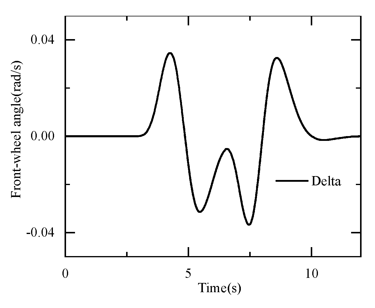
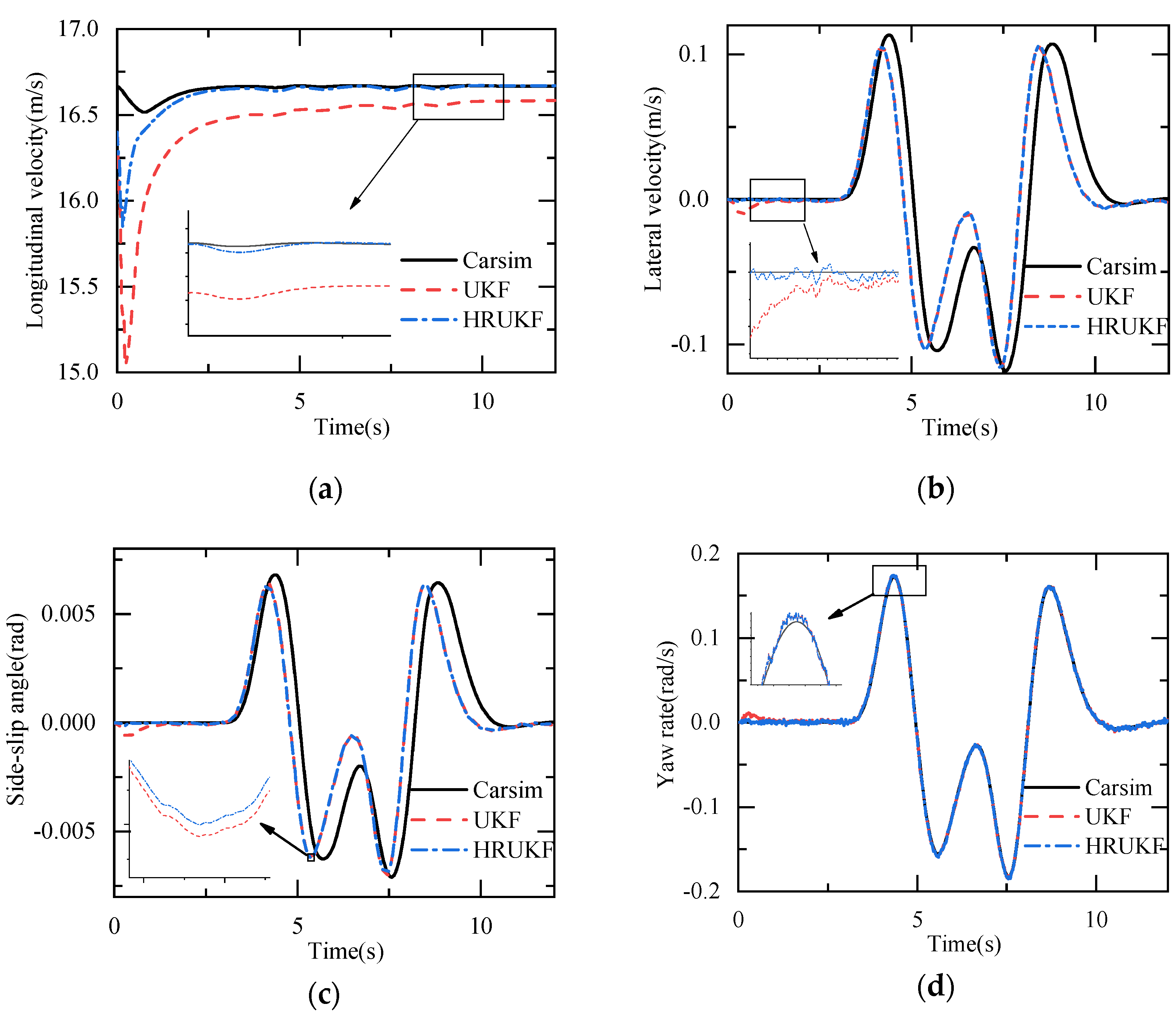
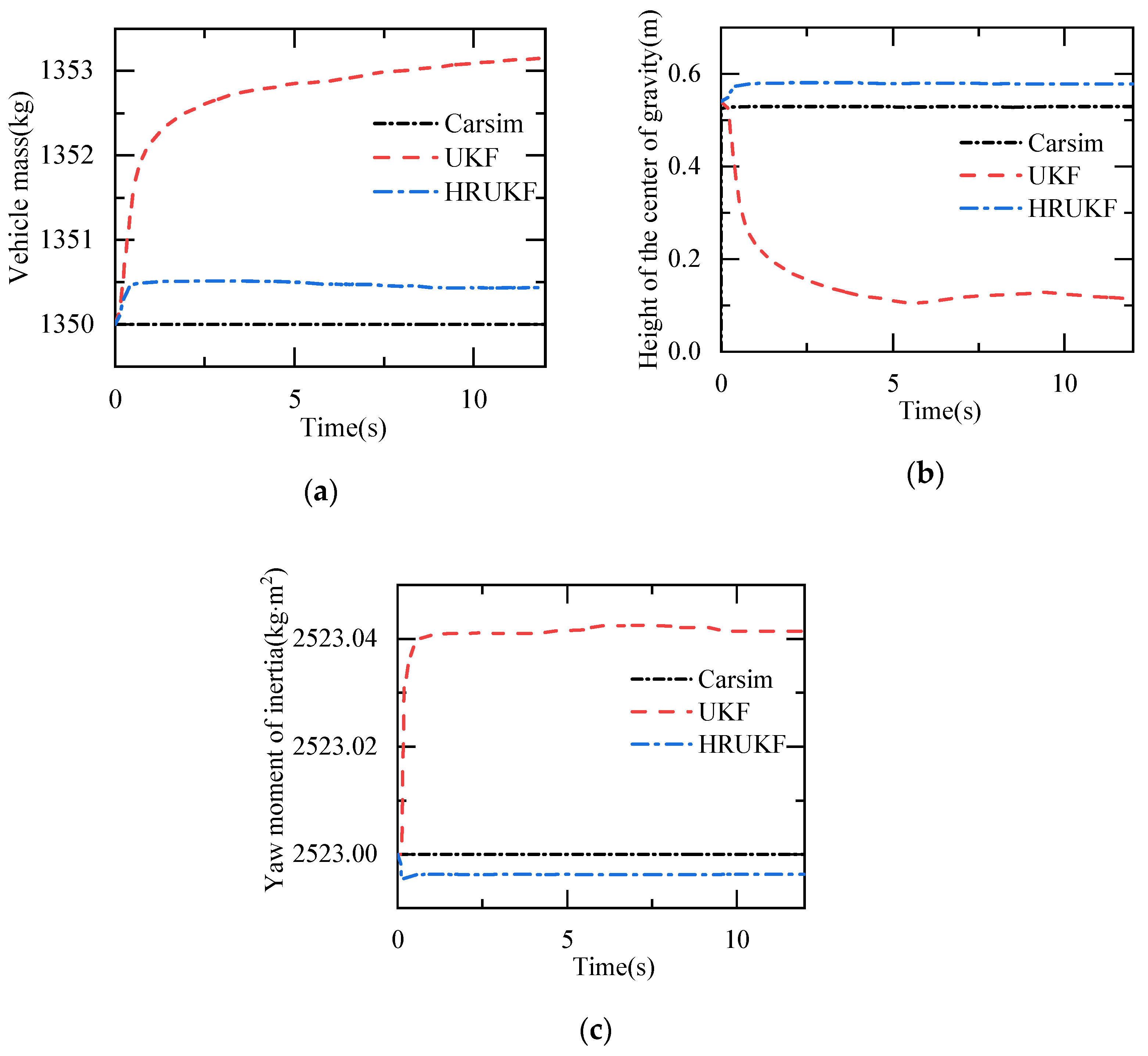
4.1. Simulation of Double-Lane Change Conditions

To evaluate the observation effect of the HRUKF observer on the vehicle state parameters, the steering condition was adopted as the double-lane change condition with more intense driving; the vehicle front wheel angle is shown in Figure 3. The wheel angle and the angular velocity of four wheels were taken as the inputs of the observer system, and the simulation results of the corresponding UKF algorithm and HRUKF algorithm were compared, as shown in Figure 4 and Figure 5.

It can be seen from the observations of longitudinal and lateral velocity, yaw rate, and sideslip angle that HRUKF can closely approximate the true value of the state output by Carsim, and HRUKF does not show large deviations in the entire double-lane change simulation. In the observations of lateral velocity, yaw, and vehicle sideslip angle, a discrete increase in the error occurred at 0–1 s. HRUKF suppressed the influence of this error, and the algorithm showed good robustness. The measurement noise of the UKF algorithm is initially set at a fixed value and cannot be updated in real-time, so the traditional UKF is less resistant to noise than the HRUKF algorithm. The reason for the error of the lateral velocity and the vehicle sideslip angle compared with Carsim is that the vehicle mathematical model is simplified compared with the simulated dynamics model, ignoring the influence of the suspension on the vehicle motion state and not considering the influence of the roll on the whole vehicle. Furthermore, the vehicle steering angle is larger under the high-speed operating conditions of the double-lane change, and there is load transfer, and the suspension has an important role in resisting load transfer. Therefore, the simplified model leads to the error of simulation results, and the accuracy of tire modeling also has an impact on the result.

According to the observation results in Figure 5, in the mass observation, the HRUKF algorithm converges to a steady-state in about 0.5 s and can estimate the true mass of the vehicle. By comparison, the UKF algorithm gradually deviates, with a mass error of about 3 kg at the end of the double-lane change condition. In Figure 5, the percentage error of the UKF algorithm in the observation of mass center height is about 280%, which does not reflect the real vehicle condition; by comparison, the HRUKF algorithm controls the error to about 10%, which better reflects the mass center height of the vehicle. Both the UKF and HRUKF algorithms can better observe the variation of inertia in the transverse pendulum rotation, and the HRUKF algorithm is closer to the true value than the UKF algorithm. To further evaluate the estimation effect of the two algorithms, the root mean square error (RMSE) was used for quantitative analysis, and was calculated as follows:

$${\mathrm{RMSE}}_k(i)=\sqrt{\frac{1}{M}{\displaystyle \sum _{l=1}^M{(x_k^{(l)}(i)-{\widehat{x}}_{k|k}^{(l)}(i))}^2}}$$

(57)

The calculated RMSE indicators under the double-lane change condition are shown in

Table 2. Root mean square error (RMSE) index for double-lane change conditions.

RMSE	Parameters	UKF	HRUKF
	Yaw rate	0.0024	0.0017
	Longitudinal velocity	0.3132	0.1092
	Lateral velocity	0.0296	0.0297
	Vehicle sideslip angle	0.0018	0.0018
	Vehicle mass	2.7951	0.4677
	Yaw moment of inertia	0.0411	0.0037
	Height of the center of gravity	0.3868	0.0500

.

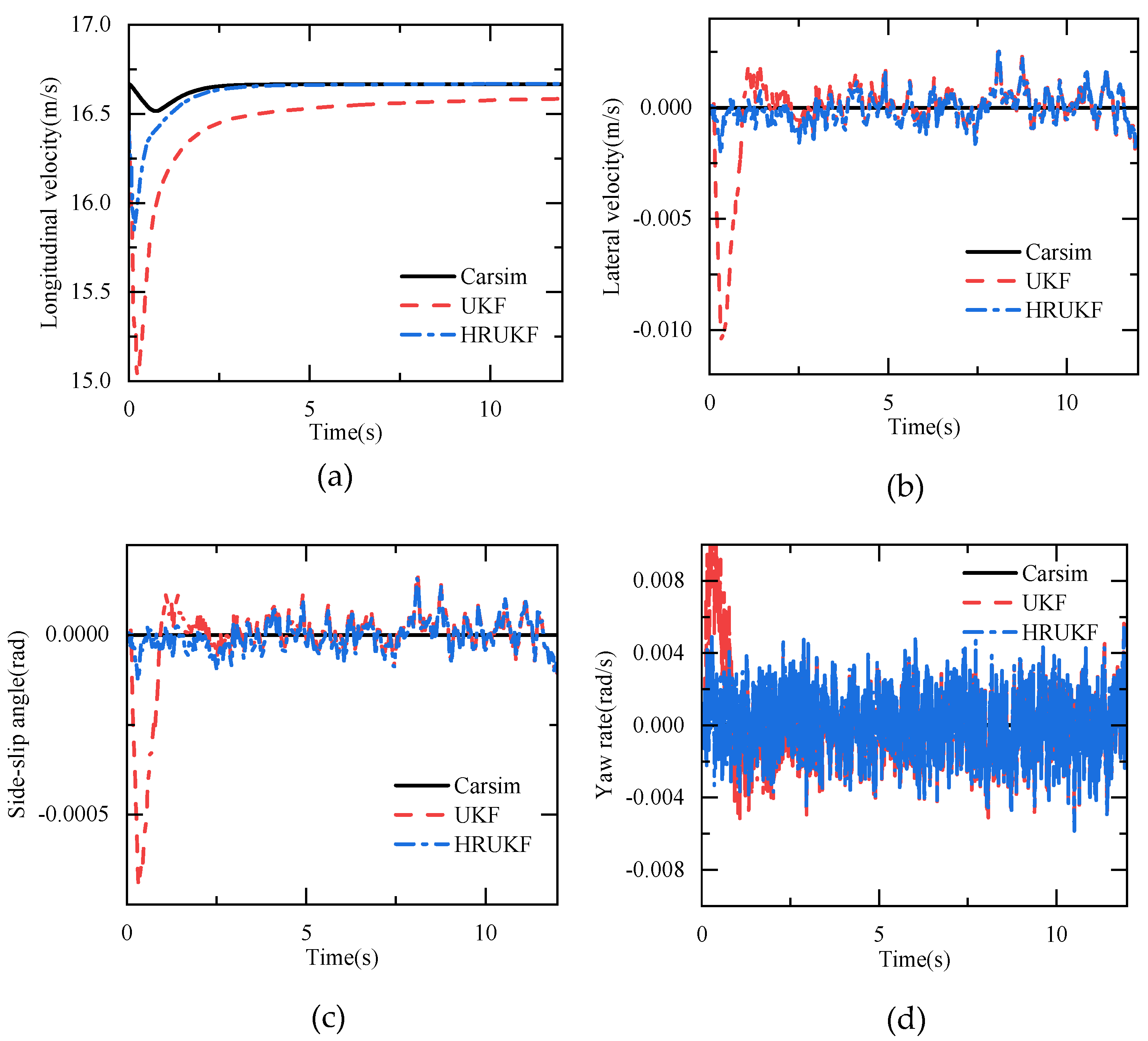
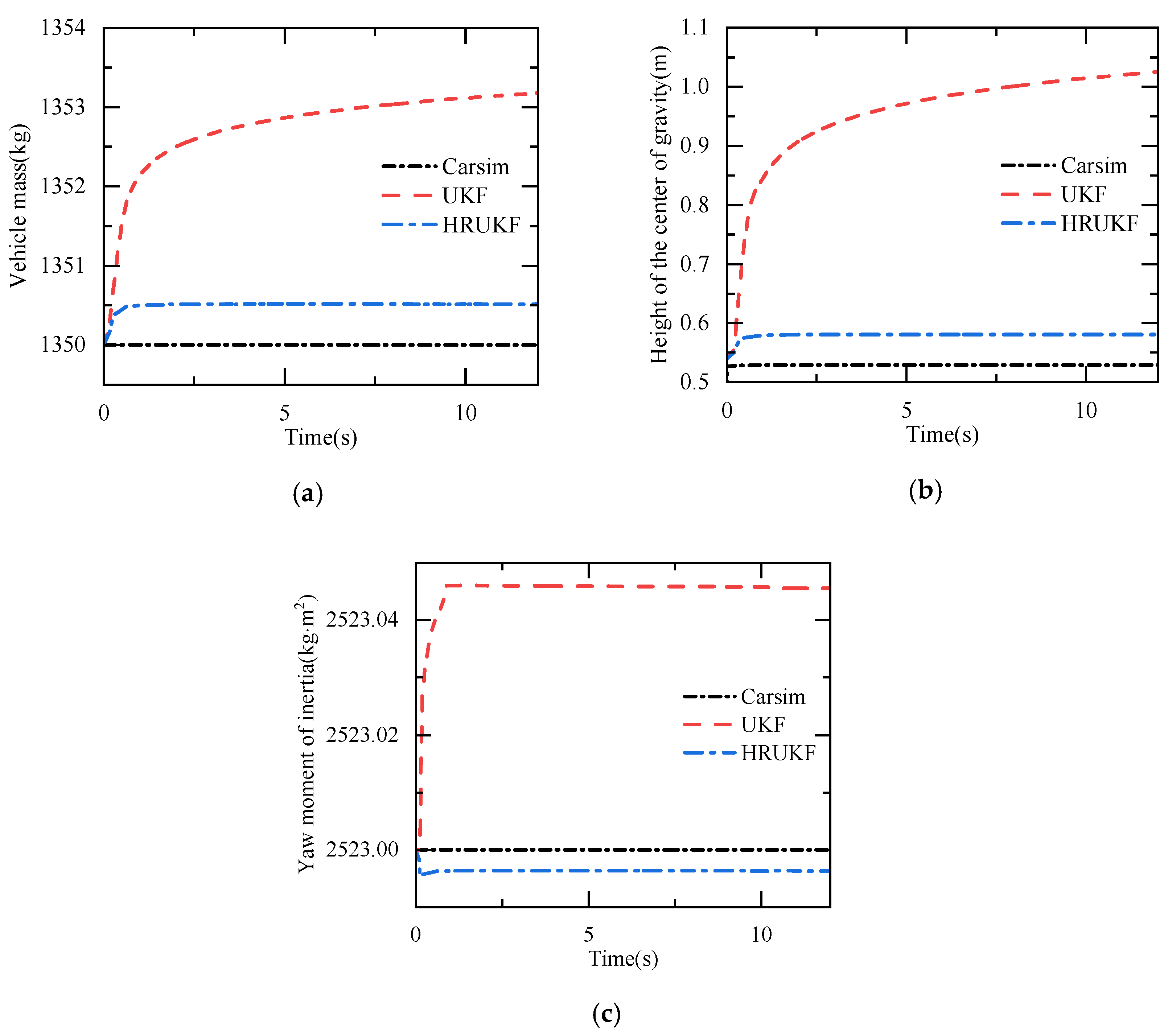
4.2. Simulation of Straight-Line Driving Condition at Constant Speed Condition

To further evaluate the observation effect of the HRUKF observer when the vehicle is driven under multiple working conditions, a 60 km/h uniform velocity driving condition was used for evaluation, with the front wheel angle constant at 0. The HRUKF and UKF algorithms are compared with the real value of the Carsim output, and the corresponding simulation results are shown in Figure 6 and Figure 7.

As shown in Figure 6, both the UKF and HRUKF algorithms experienced errors relative to the real value of the Carsim output at the beginning of the simulation in the straight-line driving condition at constant speed. However, the HRUKF had a smaller error than the UKF and converged quickly to the real value of the Carsim output in about 2.5 s, whereas the UKF algorithm converged to a certain error relative to the real value. Thus, the HRUKF algorithm can better reflect the real longitudinal speed of the vehicle under this working condition. The observation results of lateral velocity, vehicle sideslip angle, and yaw rate show that the three values of Carsim output are constant at 0 because of the uniform linear driving condition. The UKF and HRUKF incurred errors due to the influence of observation noise, and the UKF algorithm generated more errors than the HRUKF algorithm in the first 0–1 s of operation. The maximum error was more than 200%, and the HRUKF observer showed better robustness because the Huber cost function suppresses the errors generated by noise.

As shown in Figure 7, the vehicle mass observation result of the UKF algorithm gradually shifts the real value under the uniform linear driving condition. By comparison, the HRUKF algorithm converges to near the real value in about 0.5 s, and the absolute error value is about 0.5 kg, which is the same as that under the double-lane change condition. In addition, the height of the center of gravity and the yaw moment inertia observations show that the HRUKF algorithm still suppresses the outliers better with the same initial values, whereas the UKF algorithm is affected by the outlier divergence. This is particularly obvious in the height of the center of gravity observations. The results show that the Huber cost function can suppress the errors well, and HRUKF has better robustness. Similarly, to quantitatively analyze the estimation effects of the two algorithms, the RMSE indicator was used for evaluation, and the results are shown in

Table 3. RMSE index for straight-line driving condition at constant speed.

RMSE	Parameters	UKF	HRUKF
	Yaw rate	0.0023	0.0016
	Longitudinal velocity	0.3130	0.1090
	Lateral velocity	0.0019	0.0007
	Vehicle sideslip angle	0.0001	0.0004
	Vehicle mass	2.8115	0.5057
	Yaw moment of inertia	0.0451	0.0037
	Height of the center of gravity	0.4343	0.0513

.

According to the above indexes, the Huber-based robust unscented Kalman filter can well observe the state vector and the parameters of the vehicle mass, the height of the center of gravity, and the yaw moment inertia during the vehicle driving process under double-lane change and uniform velocity driving conditions.

5. Conclusions

To improve the accuracy and robustness of state observation for distributed drive electric vehicles with time-varying parameters, a robust unscented Kalman filter state observer based on the Huber method is proposed in this paper. The UKF algorithm is used to estimate all vehicle state parameters, and the Huber method is introduced to simultaneously correct for the measurement noise covariance to reduce the effect of noise uncertainty. A co-simulation using MATLAB/Simulink and Carsim was used to validate the observer for the double-lane change and straight-line driving conditions at constant speed. The HRUKF algorithm provides a good approximation of the true value of the Carsim output for longitudinal, lateral velocity, and yaw rate observations. In the observation of vehicle parameters, HRUKF quickly converges to near the true value of Carsim, and the absolute error is smaller than that of the conventional UKF algorithm. The Huber cost function can suppress the influence of outliers and noise in the case of large errors and is consistent with the UKF observations in the case of small errors, i.e., the algorithm has good robustness in both operating conditions. The results show that the HRUKF algorithm is capable of estimating vehicle state vectors and parameters, and effectively reduces the influence of anomaly errors and noise, providing more reliable observation information for vehicle stability control systems.

Therefore, future research will involve building a hardware-in-the-loop vehicle state observation simulation platform to study the effect of the method on state parameter estimation for vehicle models with more degrees of freedom, and to further verify the practical effect of the algorithm through hardware-in-the-loop simulation and real vehicle tests.

References

1. Chen, J.; Jia, G.; Yang, C. UKF-based adaptive variable structure observer for vehicle sideslip with dynamic correction. IET Control Theory Appl. 2016, 10, 1641–1652. [Google Scholar] [CrossRef]
2. Jin, X.J.; Yin, G. Estimation of lateral tire–road forces and sideslip angle for electric vehicles using interacting multiple model filter approach. J. Frankl. Inst. 2015, 352, 686–707. [Google Scholar] [CrossRef]
3. Wang, S.; Yu, Q.; Zhao, X. Vehicle sideslip angle estimation based on SVD-UPF algorithm. J. Intell. Fuzzy Syst. 2019, 37, 1–11. [Google Scholar] [CrossRef]
4. Huang, B.; Wu, S.; Fu, X. State estimation of four-wheel independent drive electric vehicle based on adaptive unscented Kalman filter. Int. J. Electr. Hybrid Veh. 2017, 9, 151. [Google Scholar] [CrossRef]
5. Wielitzka, M.; Dagen, M.; Ortmaier, T. Joint unscented Kalman filter for state and parameter estimation in vehicle dynamics. In Proceedings of the 2015 IEEE Conference on Control Applications (CCA), Sydney, NSW, Australia, 21–23 September 2015; pp. 1945–1950. [Google Scholar]
6. Jiang, K.; Victorino, A.C.; Charara, A. Adaptive Estimation of Vehicle Dynamics through RLS and Kalman Filter Approaches. In Proceedings of the 2015 IEEE 18th International Conference on Intelligent Transportation Systems—(ITSC 2015), Gran Canaria, Spain, 15–18 September 2015. [Google Scholar]
7. Hong, S.; Lee, C.; Borrelli, F. A Novel Approach for Vehicle Inertial Parameter Identification Using a Dual Kalman Filter. IEEE Trans. Intell. Transp. Syst. 2015, 16, 151–161. [Google Scholar] [CrossRef]
8. Boada, B.L.; Garcia-Pozuelo, D.; Boada, M.J.L. A Constrained Dual Kalman Filter Based on pdf Truncation for Estimation of Vehicle Parameters and Road Bank Angle: Analysis and Experimental Validation. IEEE Trans. Intell. Transp. Syst. 2017, 18, 1006–1016. [Google Scholar] [CrossRef] [Green Version]
9. Seung, J.H.; Atiya, A.F.; Parlos, A.G. Identification of unknown parameter value for precise flow control of Coupled Tank using Robust Unscented Kalman filter. Int. J. Precis. Eng. Manuf. 2017, 18, 31–38. [Google Scholar] [CrossRef]
10. Biase, F.D.; Lenzo, B.; Timpone, F. Vehicle Sideslip Angle Estimation for a Heavy-Duty Vehicle via Extended Kalman Filter Using a Rational Tyre Model. IEEE Access 2020, 8, 142120–142130. [Google Scholar] [CrossRef]
11. Huber, P.J. Robust Estimation of a Location Parameter. Ann. Math. Stats 1964, 35, 73–101. [Google Scholar] [CrossRef]
12. Chang, L.; Hu, B.; Chang, G. Huber-based novel robust unscented Kalman filter. IET Sci. Meas. Technol. 2012, 6, 502–509. [Google Scholar] [CrossRef]
13. Hou, J.; He, H.; Yang, Y.; Gao, T.; Zhang, Y. A Variational Bayesian and Huber-Based Robust Square Root Cubature Kalman Filter for Lithium-Ion Battery State of Charge Estimation. Energies 2019, 12, 1717. [Google Scholar] [CrossRef] [Green Version]
14. Xiong, L.; Shen, J.; Bi, X. A Huber based Unscented Kalman Filter Terrain Matching Algorithm for Underwater Autonomous Vehicle. In Proceedings of the 3rd International Conference on Computer Science and Application Engineering, Sanya, China, 22–24 October 2019. [Google Scholar]
15. Wang, S.; Zhang, W.; Yin, C. Huber-based Unscented Kalman Filters with the q-gradient. IET Sci. Meas. Technol. 2017, 11, 380–387. [Google Scholar] [CrossRef]
16. Liu, H.; Hu, F.; Su, J. Comparisons on Kalman-Filter-Based Dynamic State Estimation Algorithms of Power Systems. IEEE Access 2020, 1, 99. [Google Scholar] [CrossRef]
17. Li, Y.; Hou, L.; Yang, Y. Huber’s M-Estimation-Based Cubature Kalman Filter for an INS/DVL Integrated System. Math. Probl. Eng. 2020, 2020, 1060672. [Google Scholar]
18. Yu, A.; Liu, Y.; Zhu, J. An Improved Dual Unscented Kalman Filter for State and Parameter Estimation. Asian J. Control 2015, 18, 1427–1440. [Google Scholar] [CrossRef]
19. Liu, Y.H.; Li, T.; Yang, Y.Y. Estimation of tire-road friction coefficient based on combined APF-IEKF and iteration algorithm. Mech. Syst. Signal Process. 2017, 88, 25–35. [Google Scholar] [CrossRef]
20. Li, K.; Luo, Y.; Chen, H. State Estimation and Identification of Advanced Electric Vehicles; China Machine Press: Beijing, China, 2019; pp. 28–30. [Google Scholar]
21. Dakhlallah, J.; Imine, H.; Sellami, Y. Heavy vehicle state estimation and rollover risk evaluation using Kalman Filter and Sliding Mode Observer. In Proceedings of the 2007 European Control Conference (ECC), Kos, Greece, 2–5 July 2007. [Google Scholar]
22. Liu, X.; Deng, X.; He, Y.; Zheng, X.; Zeng, G. A Dynamic State-of-Charge Estimation Method for Electric Vehicle Lithium-Ion Batteries. Energies 2020, 13, 121. [Google Scholar] [CrossRef] [Green Version]
23. Gao, Z.; Chen, S.; Zhao, Y.; Nan, J. Height Adjustment of Vehicles Based on a Static Equilibrium Position State Observation Algorithm. Energies 2018, 11, 455. [Google Scholar] [CrossRef] [Green Version]
24. Zahid, T.; Li, W. A Comparative Study Based on the Least Square Parameter Identification Method for State of Charge Estimation of a LiFePO4 Battery Pack Using Three Model-Based Algorithms for Electric Vehicles. Energies 2016, 9, 720. [Google Scholar] [CrossRef] [Green Version]
25. Wang, Z.; Wu, J.; Zhang, L. Vehicle sideslip angle estimation for a four-wheel-independent-drive electric vehicle based on a hybrid estimator and a moving polynomial Kalman smoother. Proc. Inst. Mech. Eng. Part K J. Multi-Body Dyn. 2018, 233, 125–140. [Google Scholar] [CrossRef]
26. Zhao, J.; Mili, L. Robust Unscented Kalman Filter for Power System Dynamic State Estimation with Unknown Noise Statistics. IEEE Trans. Smart Grid 2019, 10, 1215–1224. [Google Scholar] [CrossRef]
Figure 1. The non-linear three-degrees-of-freedom (3-DOF) vehicle model.
Energies 14 00750 g001
Figure 2. Diagram of Huber-based robust unscented Kalman filter (HRUKF) process.
Energies 14 00750 g002
Figure 3. Front-wheel angle.
Energies 14 00750 g003
Figure 4. Vehicle state vector observation results under double-lane change condition. (a) longitudinal observation results; (b) lateral velocity observation results; (c) side-slip angle observation results; (d) yaw rate observation results.
Energies 14 00750 g004
Figure 5. Observation results of vehicle parameters under double-lane change condition. (a) vehicle mass observation results; (b) height of the center of gravity observation results; (c) yaw moment of inertial observation results.
Energies 14 00750 g005
Figure 6. Observation results of vehicle parameters under the straight-line driving condition at constant speed condition. (a) longitudinal velocity observation results; (b) lateral velocity observation results; (c) side-slip angle observation results; (d) yaw rate observation results.
Energies 14 00750 g006
Figure 7. Observation results of vehicle parameters under the straight-line driving condition at constant speed. (a) vehicle mass observation results; (b) height of the center of gravity observation results; (c) yaw moment of inertial observation results.
Energies 14 00750 g007