Article

Effectiveness Analysis of PMSM Motor Rolling Bearing Fault Detectors Based on Vibration Analysis and Shallow Neural Networks

by
Pawel Ewert
*,
Teresa Orlowska-Kowalska
and
Kamila Jankowska
Department of Electrical Machines, Drives and Measurements, Wroclaw University of Science and Technology, Wybrzeze Wyspianskiego 27, 50-370 Wroclaw, Poland
*
Author to whom correspondence should be addressed.
Energies 2021, 14(3), 712; https://doi.org/10.3390/en14030712
Submission received: 12 December 2020 / Revised: 25 January 2021 / Accepted: 27 January 2021 / Published: 30 January 2021
(This article belongs to the Special Issue Fault Diagnosis of Electrical Machines and Drives)

Abstract

:
Permanent magnet synchronous motors (PMSMs) are becoming more popular, both in industrial applications and in electric and hybrid vehicle drives. Unfortunately, like the others, these are not reliable drives. As in the drive systems with induction motors, the rolling bearings can often fail. This paper focuses on the possibility of detecting this type of mechanical damage by analysing mechanical vibrations supported by shallow neural networks (NNs). For the extraction of diagnostic symptoms, the Fast Fourier Transform (FFT) and the Hilbert transform (HT) were used to obtain the envelope signal, which was subjected to the FFT analysis. Three types of neural networks were tested to automate the detection process: multilayer perceptron (MLP), neural network with radial base function (RBF), and Kohonen map (self-organizing map, SOM). The input signals of these networks were the amplitudes of harmonic components characteristic of damage to bearing elements, obtained as a result of FFT or HT analysis of the vibration acceleration signal. The effectiveness of the analysed NN structures was compared from the point of view of the influence of the network architecture and various parameters of the learning process on the detection effectiveness.

1. Introduction

Today, permanent magnet synchronous motors (PMSMs) are gaining more popularity in industrial applications. They are also willingly used in the drive systems of electric and hybrid vehicles. This is due to their numerous advantages, such as high efficiency, possibility of high torque overload, and high power-to-weight ratio. They work well in applications that require both high precision and high dynamics [1,2]. Reliability is an equally important requirement for a modern drive system. Very good operating parameters do not make the PMSM failure-free. The factors causing different damages may include: too high of a current flow, high operating temperature, inadequate lubrication, or corrosion [2]. The introduction of diagnostics of the drive system enables the detection of damage to motor components already in the initial stage of their development. Usually, the failure of one of the components leads to subsequent failures. Monitoring allows you to plan the replacement of the damaged part and prevent failure of subsequent components. Appropriate diagnostics guarantees safety and extends the service life of the machine [3]. The rolling bearings discussed in this article are the most damaged components of the AC (alternating current) motors of medium power. They account for about 40% of all failures in electrical machines, while stator, rotor, and other failures account 36%, 9%, and 14%, respectively [4]. Rolling bearings are responsible for maintaining a constant air gap between the rotor and the stator. Therefore, their failure gradually leads to the failure of the entire machine [3,4].
There are many methods for diagnosing AC motor bearings. When detecting this type of damage, vibrations are most often used as a diagnostic signal [5]. Other popular carriers of failure symptoms are current [6], speed [7], noise [8], and temperature [9]. The Fast Fourier Transform (FFT) was used in [3] as one of the methods that can be used for the pre-processing of the stator current for diagnostic purposes. The method requires that the processed signal is stationary, which is difficult to achieve in a variable speed drive system. Therefore, in References [3] and [10], for transient states (under load torque change), the increasingly popular wavelet decomposition was used. In Reference [11], the less frequently used Variational Mode Decomposition (VMD) method is presented, which allows for the separation of the vibration signal components important in the diagnostics process from those disturbing this process. The Hilbert transform (HT) was used to increase the stability of the detection with VMD method.
More often, authors compare the possibility of detecting rolling bearing damages using several diagnostic signals. For example, in Reference [12], three diagnostic signals were tested: stator current, rotor speed, and mechanical vibrations. The symptoms were extracted using FFT and the kurtosis spectrum analysis, which improves the signal-to-noise ratio. The tests included the influence of different values of rotational speed and the change of the load torque. Another approach consists in the comparative analysis of several methods of processing one diagnostic signal. In Reference [13], the authors analysed the vibration acceleration signal to detect the damage to rolling bearings in Brushless Direct Current Motor (BLDCM) drive. In the presented research, the possibility of detecting a damaged bearing was assessed using four methods of signal processing: classical FFT of the signal, Fourier transform from the absolute value of the signal, Fourier transform from the envelope signal calculated using the Hilbert transform, and Fourier transform from the signal filtered by the Teager–Kaiser energy operator. The results were presented for three different cases of rolling bearing failures and compared with an undamaged bearing. Authors showed that the use of an additional signal processing method, based on the Hilbert transform, TKEO (Teager–Kaiser energy operator) filter or the absolute value transform, allows to better monitor bearing condition. The relative amplitude of the observed characteristic frequencies increased several dozen or several hundred times, and in the case of TKEO, even several thousand times, which simplified the fault recognition.
As the mechanical structure of AC motors (IMs, PMSMs, BLDCMs) are different, the structure resonances are also different. Thus, the amplitudes of the same fault can vary from machine to machine and we will get different amplitude values at different harmonic numbers describing the specific bearing. However, the methodology of fault diagnosis will be the same for rolling bearings of different machines [2,5,13,14]. The main task of the diagnostic system designer is to select those harmonics, which are most sensitive to selected fault types for a given drive system.
The use of any of the above-mentioned signal processing methods to the mechanical and/or electrical signals carrying symptoms of bearing failures requires the analysis and evaluation of the obtained results. The expert knowledge is required to use these symptoms in diagnostic process, to interpretation of the results, to setting the suitable thresholds and to carry out regular monitoring of these analyses. This type of approach introduces a human factor that reduces the fault tolerance of the entire system. Therefore, methods are being sought to eliminate this human factor and automate the detection process. At present, this task is more often performed by neural networks (NNs), which can act as detectors and/or classifiers of damages, minimizing human participation in the diagnostic process [1,5,14,15,16,17,18,19,20,21,22,23].
Recently, in the research on the detection of damage to rolling bearings in AC motor drives, frequently, deep neural networks (DNNs) are proposed, which are gaining more popularity due to the development of deep learning methods [1,15,16]. In Reference [1], the diagnostics of rolling bearings of the PMSM drive using a convolutional neural network (CNN) was presented, based on the measurement of stator current and vibration signals. Simultaneous analysis of stator current frequency spectrum and raw vibration signal allowed obtaining detection efficiency at the level of 96%. Diagnostics based on one measured signal only led to the efficiency on a two-fold lower level. In Reference [15], the deep autoencoder based unsupervised learning method was used to classify three states of the PMSM motor: undamaged, bearing outer-race fault, and 10% inter-turn short circuit fault. The Continuous Wavelet Transformation (CWT) was used for the initial signal processing of the stator current and mechanical vibration signals. The authors obtained the classification accuracy with the simultaneous use of both signals at the level of approximately 91% for signals without noise and approximately 88% for signals with noise. The classifier based only on the current signal achieved a detection accuracy of approximately 99% (signal without noise) and approximately 75% for a signal with noise, while based on mechanical vibrations, approximately 69% and approximately 66%, respectively. Authors of [16] present a classifier of three states of the PMSM motor: undamaged, bearing outer-race fault, and 10% inter-turn short circuit fault. In this case, the motor operated under conditions of variable speed and variable load torque. The stator current and mechanical vibrations were analysed, and the classification was carried out by a Support Vector Machine with the Gaussian radial basis function (RBF) as the kernel in the Support Vector Machine (SVM). The obtained accuracy of this SVM classifier was approximately 93%.
The growing interest of scientists in deep neural networks has resulted in a much smaller number of articles using classic shallow neural networks (NNs) in the PMSM drive diagnostics. However, classic NNs have several important advantages that should be taken into account, such as simpler architecture, shorter learning time and therefore lower computational complexity, including lower requirements on the power of processors during practical implementation.
It needs to be highlighted that a properly parameterized classic NN allows for a very high level of efficiency in electric machine diagnostics. An example of such a network is the multilayer perceptron (MLP) used in Reference [17], where authors present the use of networks with one hidden layer, learned with the delta rule algorithm to detect eccentricity and damage to rolling bearings in the PMSM. Stator current was used as a diagnostic signal. The effectiveness was tested for variable speed and load torque values. The problem was treated in a binary way, thus the network response showed only failure (1) or healthy (0) operating conditions. The best results, 100% efficiency, was obtained for the highest load and speed values.
Self-organizing maps (SOMs), also known as Kohonen Neural Network (KNN), were also used as damage classifiers of rolling bearings. The bearing fault diagnosis using SOM was presented, e.g., in Reference [5]. In this work, the diagnostics was based on vibration measurement. FFT and wavelet transform were used for the initial signal processing. The task of the NN was the fault level classification. The research was conducted for five different loading conditions, five different shaft speeds and eight bearing failures. The proposed SOM made it possible to detect a damaged bearing with a low topological error of about ± 0.04, but a moderate quantisation error of ± 0.5.
An example of a very extensive classical NN can be found in Reference [22]. The authors developed three-layer MLPs with 10, 15, 20, 25, 30, and 35 neurons in the hidden layer, respectively. In addition to the two amplitudes of characteristic frequencies of the damage, the amplitude of the rotational frequency, the Kurtosis factor of the vibration waveform, and the maximum and average values of the vibration signals are applied for the inputs of these NNs. The neural network had three outputs, each one serving as an indicator for one of the three faults: bearing looseness, defects on the inner raceway, and defects on the rolling element. At the output information about the technical condition of the tested bearing element was obtained (damaged or not). The Levenberg–Marquardt algorithm was used for training supported by cross-validation method to improve generalization and to avoid overtraining. Despite relatively larger number of neurons in the hidden layer, the presented detectors were characterized by an average efficiency of approximately 86–96%. Another example of using classic NNs consists in expanding the number of network inputs [23]. The authors used measurement data from the Bearing Data Center of Case Western Reserve University to train a Self-Organizing Map (SOM) to classify damages to rolling bearings. Differences of 70 features, such as statistical features, frequency domain features, autoregressive model coefficients, wavelet packet decomposition analysis, and empirical mode decomposition entropy energy were used as SOM inputs. Two techniques were used to select the optimal features (extended relief and min redundancy max relevance (mRMR) algorithms), which allowed to obtain as much as 100% effectiveness for 33 features. However, a practical realisation of such extended fault detectors or classifiers is rather difficult, especially when you want to use simple processors, e.g., ARM type and applied such solutions in industry.
Although, as can be seen from the above literature overview, there are examples of the use of selected classic NN structures for the diagnostics of rolling bearings in variable speed PMSM drives, there is a lack of comparison of the effectiveness of various neural structures in the detection and/or classification of bearing failures carried out for a wide range of operating conditions of such a drive.
Hence, the aim of this study is a comparative analysis of the effectiveness of three selected types of NNs for the detection of damage to rolling bearings in PMSM drive. Two methods of vibration signal processing were used to obtain diagnostic symptoms: fast Fourier transform (FFT) and Hilbert transform (HT) to obtain the envelope signal, which was next subjected to FFT analysis. The preliminary analysis allowed distinguishing several diagnostic symptoms characteristics for the failure of rolling bearings. The article presents and compares the possibility of using MLPs, RBF networks, and Kohonen maps for detection and classification of bearing damages. Two variants of the NN detector operations were analysed: the first one determined whether there was damage or not (fault detector), the second one identified the type of damaged structural element of the bearing (fault classifier). In addition, in this article, the impact of NN topology, activation function, learning method and learning rate on the detection/classification efficiency was analysed. It was assumed that developed neural detector and classifiers should achieve accuracy at the level of 95–100%, but not less than 90%. The article presents selected results of the operation of the developed and tested neural detectors of rolling bearings based on vibration acceleration signals acquired in the laboratory set-up with PMSM drive.
The first part of the article contains a review of the literature on the diagnosis of rolling bearings, with particular emphasis on PMSM drives, and the motivation of the research presented. In the following two sections, the characteristics of the damage to rolling bearings and the methods used for the initial signal analysis are discussed. In the fourth section, the applied NN structures are shortly characterized. In the fifth section, the experimental test results of the shallow NN-based rolling bearing fault detectors and classifiers are presented. These tests were carried out with the use of FFT and HT as pre-processing methods applied for selecting the most significant symptoms of the vibration acceleration signals for analysed NN structures with different architectures and parameters. The article ends with a short conclusion and summary of the results obtained.

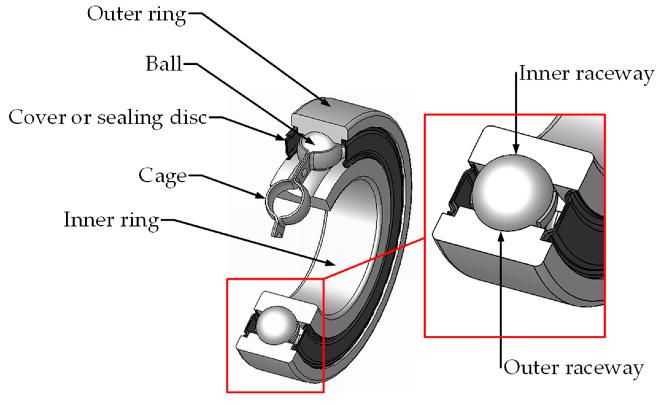
2. Brief Characteristic of Bearing Failure Symptoms

Rolling bearings are elements of a drive enabling rotation of the rotor with minimal mechanical losses. The bearings allow minimizing the resistance to movement of the shaft and keep it in the right position. Therefore, bearings are the elements most intensively subject to the wear process [3,4]. In general, rolling bearings consist of a cage in which the rolling elements are placed and properly separated. The cage is located between the inner ring, which is placed on the machine shaft, and the outer ring [21]. The rolling bearing structure is shown in Figure 1.
Due to their nature, damage to rolling bearings can be divided into two types [24,25]:
  • Point damages (cavities, splinters of small fragments);
  • Diffuse damages (surface deformation, corrosion damage, unevenness).
Both types of damages lead to different symptoms. Point damages cause vibrations in the low frequency range. Diffuse damages are detected by observing the vibration spectrum over a wide range. Due to their nature, they are difficult to describe in terms of specific frequencies. The occurrence of damage and its further deepening causes a change in the geometry of the rolling elements, an increase in vibration and noise level of the motor during operation, and, along with their deterioration, may lead to the eccentricity of the rotor in relation to the stator and damage to the mechanical connection with the working machine. Like any element of the electric drive, the bearings have a long service life and their natural damage results from the nature and time of operation. Premature failures can occur for many reasons. Most often, they result from improper assembly, often they are also caused by improper selection of the bearing to the drive requirements and its improper operation [26,27,28,29]. Depending on which element of the bearing is spot damaged, different damage symptoms appear in the spectrum of the mechanical vibration signal [13,21,24,25].
The symptoms defining the bearing condition are obtained by determining the amplitudes of the characteristic frequencies occurring in the vibration spectrum. A significant increase in these amplitudes indicates a point damage to a given element. To calculate the characteristic frequencies, it is necessary to find the rotational frequency fr of the motor shaft:
f r = n 60 ,  
where: n—motor velocity (rpm).
Then the frequencies characteristic harmonics for failures of individual bearing elements can be determined on the basis of the formulas below [21,22,24]:
f b c = 1 2 f r ( 1 D b D c cos β ) ,  
f o r = N b 2 f r ( 1 D b D c cos β ) ,
f i r = N b 2 f r ( 1 + D b D c cos β ) ,
f r e = D c D b f r ( 1 ( D b D c cos β ) 2 ) ,
where: Nb—number of rolling elements (balls), Db—rolling element diameter, Dc—bearing pitch diameter, β—bearing working angle (0o for rolling bearing), fbc, for, fir, fre—frequencies specific for a given failure: bearing cage, outer race, inner race, and rolling element.
It is clearly seen that frequencies of the characteristic harmonics depend only on the shaft frequency (which, in the PMSM motor, is independent on the load torque, contrary to IM) and rolling bearing geometry.

3. Methods Used for Failure Symptoms Analysis in the Vibration Signal

In this work, two methods of vibration signal analysis were used to prepare the input signals of the developed neural detectors: the classical Fast Fourier Transform (FFT) and FFT of the vibration acceleration envelope signal calculated using the Hilbert transform (ENV).

3.1. Fast Fourier Transform

Classic FFT is the transformation most often used in machine diagnostics. It converts a signal from the time domain to the frequency domain and in a continuous form can be written as follows [30]:
F ( j , ω ) = f ( t ) e j ω t d t .  
The Fourier transform assumes that the analysed signals are periodic and stationary and performs decoding of the analysed signal into a specified number of sinusoidal signals with a specified component frequency. The real signals in most cases do not meet the periodicity and stationarity conditions. In addition, the signal must be sampled synchronously with the fundamental frequency of the signal, according to Shannon’s sampling theorem. The length of the analysed signal fragment must be an integer multiple of its fundamental harmonic period. For signals that meet these criteria, the obtained spectrum is correct; otherwise, there is a blurring of the spectrum. It is also related to the inaccuracy of the amplitude determination and can have a significant influence on the interpretation of the results. The transition from the time domain to the frequency domain means that the moment of appearance of a given component does not affect its place in the spectrum. Therefore, the signal subjected to such analysis should be stationary due to the loss of time information.
The Discrete Fourier Transform (DFT) is used for signal analysis [30]:
X ( k ) = n = 0 N 1 x ( n ) e j 2 π n k N ,
where: x(n)—real discrete signals of finite length N, generated during continuous signal sampling.
The basic form used to present results after the Discrete Fourier Transform (DFT) is the frequency spectrum with harmonic magnitudes calculated according to:
| X ( k ) | = ( Re { X ( k ) } ) 2 + ( Im { X ( k ) } ) 2 .
For the purpose of scaling the spectrum in frequency units, each |X(k)| sample is attributed frequency f(k) calculated according to the following expression:
f ( k ) = k f p N ,
where: fp is the signal sampling frequency and N the number of all signal samples.

3.2. Hilbert Transform

The continuous Hilbert transform for any time course x(t) has the following form [31]:
H [ x ( t ) ] = 1 π x ( τ ) t τ d τ .
The analytical signal a(t) created from the real signal x(t) and its Hilbert transform has the following form [31]:
a ( t ) = x ( t ) + j H [ x ( t ) ] = a E N V ( t ) e j φ ( t ) ,
where: aENV(t)—instantaneous amplitude of the envelope of original signal x(t), ϕ(t)—instantaneous phase calculated as follows [31,32]:
a E N V ( t ) = x 2 ( t ) + H 2 [ x ( t ) ] ,
ϕ ( t ) = arctan H [ x ( t ) ] x ( t ) .  
Analysis of the aENV(t) signal makes it possible to find the frequencies characteristic for failures in the medium-frequency range of the spectrum. Finding the characteristic frequencies in the low-frequency range requires high frequency resolution. Obtaining the high frequency resolution requires steady-state operation of the machine, which is difficult to maintain in real conditions. A characteristic feature of the Hilbert transform application is resistance to the detection of vibrations originating from sources other than bearing damage. A signal is obtained from which the natural frequency of the diagnosed motor is also eliminated. This is a significant advantage of this transformation. HT improves the symptom extraction process, and thus the effectiveness of the diagnostic system, even in the case of significant disturbances in the measurement signal [31].

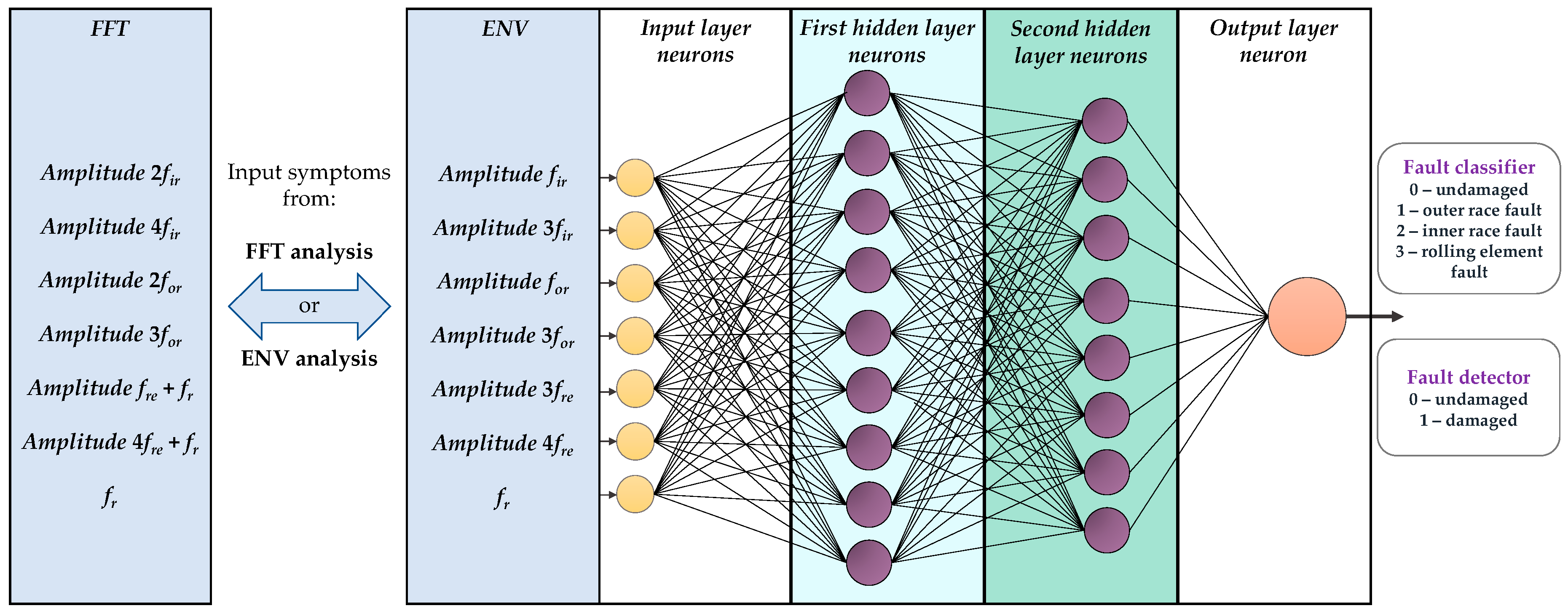
4. Neural Network Structures Used

In this study, bearing failure detectors using various structures of shallow neural networks were analysed and their effectiveness in the detection and classification of the analysed failures was compared. The following NNs were taken into account: multilayer perceptrons (MLPs), networks with radial base functions (RBFs), and self-organizing Kohonen maps (self-organizing maps, SOMs).

4.1. Multilayer Perceptrons

Feedforward MLPs are most popular in various industrial applications, and consist of the input layer, one or more hidden layers, and the output layer. Each neuron in each layer is connected to a neuron of the next layer; there are no connections between neurons of the same layer, and the data are processed in parallel. This type of NN performs a global approximation [33,34]. This means that many neurons simultaneously decide to map each element of the input vector. The structure of the MLP network with one hidden layer is shown in Figure 2.
In general, the MLP network can be described as follows:
y k = f 2 ( i = 1 M w k i ( 2 ) × f 1 ( j = 1 N w i j ( 1 ) × x j + w 0 ( 1 ) ) + w 0 ( 2 ) ) ,  
where: ykk-th output of the network, xjj-th input of the network, w i j ( 1 ) , w k i ( 2 ) weights of the first and second hidden layers, respectively, w 0 ( 1 ) , w 0 ( 2 ) —biases in the first and second hidden layers, respectively.
The MLP network training process consists of modifying weights in such a way as to minimize the objective function, usually the mean square error of the output value in relation to the expected value. In this work, the Levenberg–Marquardt (L–M) algorithm [35,36] was used to train MLP networks, which combines the iterative features of the optimization method of the Gauss–Newton algorithm, and the steepest descent algorithm. Thanks to this, we obtained a tool that works as the gradient descent, when we are far from the minimum of the objective function, and then reduces to the conjugate gradients method. The general form of the L–M learning algorithm is described by the Equation (15) [35,37,38]:
w n + 1 = w n η ( J n T J n + μ I ) 1 J n e n ,  
where: wn—weight of the network, µ—regularization factor determining the algorithm operation, Jn—Jacobian matrix, en—learning error, η—learning rate.
The difference between Newton’s formulas is adding the unit matrix multiplied by the regularization factor µ. It always has a positive value modified in the learning process. By changing this coefficient, we go continuously from the steepest descent algorithm method to the Newton unfolding method. For values close to zero, the algorithm will calculate weights in a manner similar to the unfolding method. Increasing the value of µ is accompanied by an increase in the importance of the direction of improvement determined on the basis of the error function gradient. Apart from determining the share of individual strategies in the obtained result, µ also fulfils the function of the step size towards improvement [35,37,38].
The Levenberg–Marquardt algorithm is very sensitive to initializing weight values because they are selected randomly. An improvement to the above method is the addition of Bayesian regularization. This improves the generalizing properties of the network. Regularization introduces a change to the objective function. Not only is the aim to minimize the mean square error, but also to achieve it with the lowest possible weights. The objective function takes the following form [39,40]:
C = β E + α E w ,  
where: E—sum of mean square errors, Ew—sum of squared weights, β—learning factor, α—decay rate.
The α factor enforces low weight values which greatly reduces the tendency of the network to over-fit. This modification also provides greater immunity to noise and incorrect input data, but is more time-consuming [39,40].

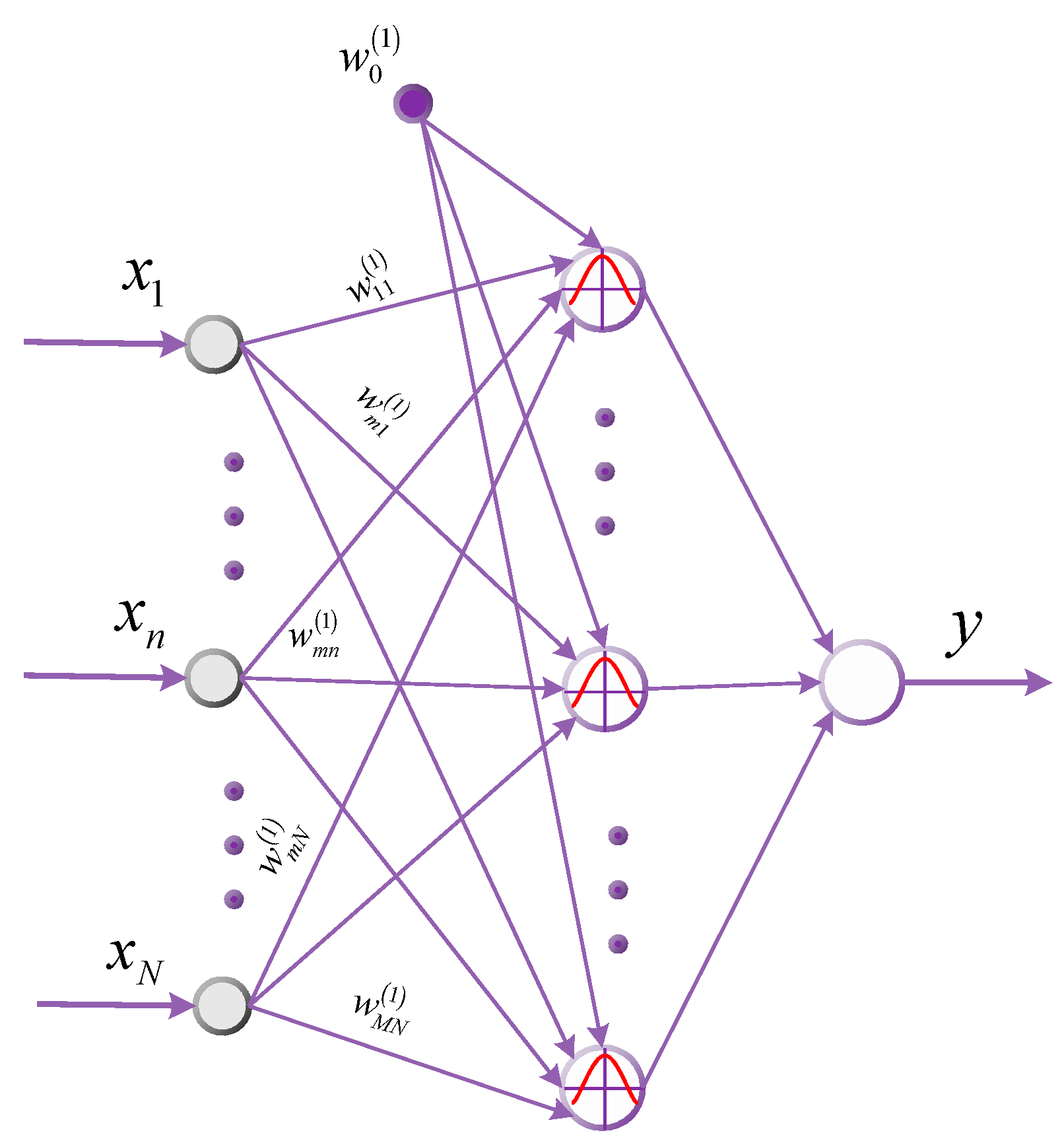
4.2. Radial Basis Networks

Another structures used in this research are radial networks (radial basis functions, RBFs), i.e., feedforward NNs with one hidden layer in which activation functions are radial. Each element of the input vector is mapped by a particular radial neuron of the hidden layer. The output layer neurons are linear and are responsible for summing the outputs of individual neurons of the hidden layer. The structure of the RBF network is shown in Figure 3.
Contrary to MLP networks, whose neurons perform the task of global stochastic approximation of functions of many variables, in RBF networks, the mapping of the full set of input data is the sum of local mappings [34]. Output values of the RBF network are obtained as a sum of product of the RBF neuron outputs and weight factors:
y k = j = 1 N w j k ϕ j + w k 0
with outputs of the RBF neurons calculated obtained as follows:
ϕ j = exp ( υ j 2 ( X ) 2 σ j 2 ) ,
where: ykk-th output of the network, wjk—weight factor between the j-th output of the hidden (RBF) layer and k-th neuron of NN output, wk0—bias of k-th output neuron, υj(X)—the Euclidean distance input vector values and centres of RBF functions, σ—is a spread factor of the activation function.
The Euclidean distances between input vector values and centres of RBF functions are calculated:
υ j ( X ) = X C j = k = 1 N ( x k c k ) 2 , k = 1 , 2 , 3 , N
where: X = [x1, x2, x3,...., xN]T is the input vector, Cj—vector related to the centre of each RBF neuron.
The design process for RBF networks is much simpler than for MLP. The learning procedure consists of three stages that include [41]:
  • Choice of the centres, Cj, of the hidden radial basis neurons;
  • Choice of the spread parameter, σ—width of the radial function for each hidden neuron;
  • Determination of the weight factors, wjk, between hidden (radial) and output layer.
The first step may be carried out randomly with even distribution. For more complicated problems, data clustering algorithms are used. The most popular is the k-means algorithm [41]. The algorithm requires top-down determination of the number of clusters. In general, the k-means algorithm aims to place the centres of RBF neurons in the areas with the most significant data [42,43]. The weights of the output layer are determined by the supervised learning method, e.g., according to the delta rule. Learning rate is much shorter and the problem of local minimum is avoided.

4.3. Kohonen Maps

The last NN structures used in this work to detect damage to rolling bearings are self-organizing maps (SOMs). Network learning is based on the built-in mechanism of competition and neighbourhood assessment. The SOM is formed by the input and output (competition) layers. The construction is less complicated than the MLP and RBF networks due to the lack of a hidden layer (Figure 4).
As for the similarities, these are also feedforward networks, and each input layer element is connected to each output layer element. The output signal yk of the k-th neuron is described by the vector relationship:
y k = W T X = W   X   cos ϕ k .
Since the input x and the weight W vectors are normalized in the network, the output value of yk (neuron activation) is determined by the angular difference φk between the vectors X and W.
Self-organizing networks allow you to find unknown connections between input data, which is possible using two learning methods: Winner Takes All (WTA) and Winner Takes Most (WTM). In the WTA method, only the winning neuron is adapted. Adaptation consists in bringing the winning neuron closer to the input pattern. The WTM algorithm assumes that also neurons from an appropriately defined neighbourhood (e.g., Gauss neighbourhood function) can be activated (weight adaptation). Usually, Euclidean distance is taken as the neighbourhood measure [44,45,46].

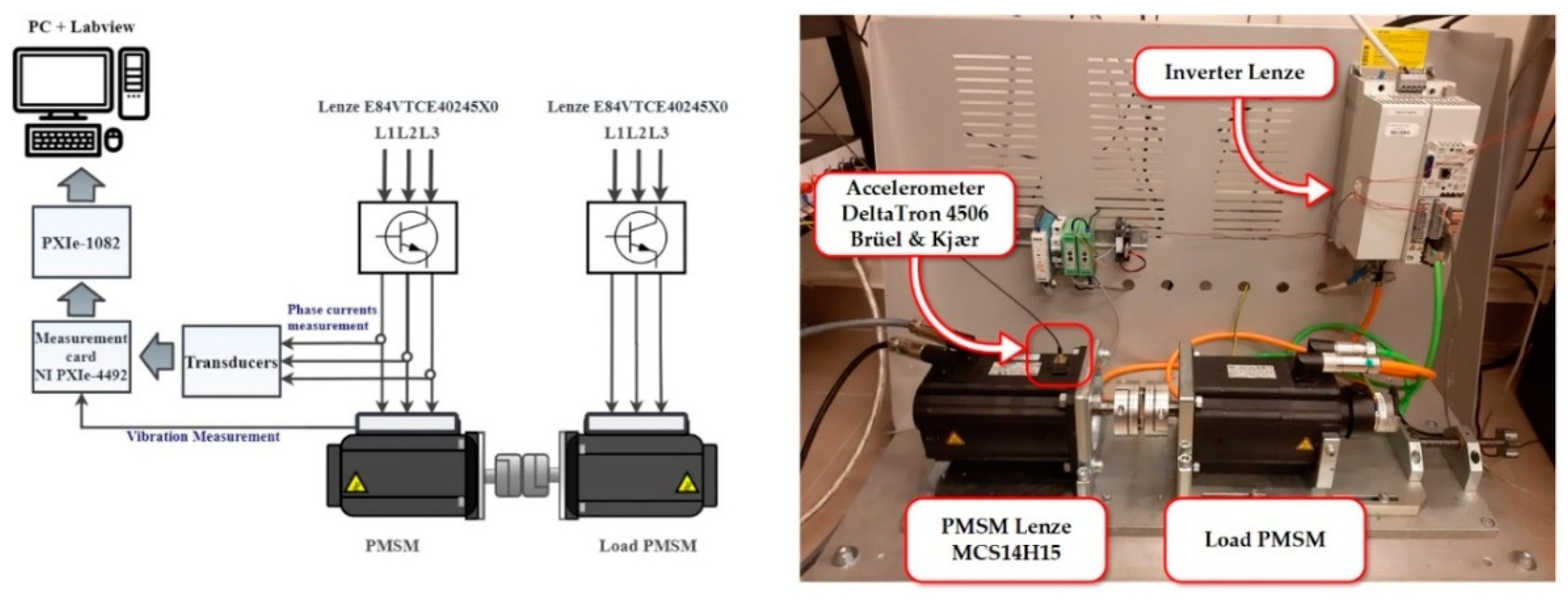
5. Description of the Laboratory Set-Up

In order to obtain training and testing data for the developed NN detectors, the vibration acceleration signal of the tested PMSM (Lenze MCS14H15), with a rated power of 2.5 kW (UN = 325 V, IN = 6.6 A, TN = 21 Nm, fs = 100 Hz, nN = 1500 rpm, pp = 2), was measured. It should be highlighted that in the presented research the original measurement data were used, obtained in laboratory set-up developed by authors, for the PMSM supplied from the industrial frequency converter operating in vector control mode, as it can be met in real industrial conditions. The authors resigned from the use of generally accessible databases, the analysis of which has been presented in numerous articles. The tested motor was powered by a 4 kW Lenze E84VTCE40245 × 0 converter. This device allows us to control the motor in one of several vector or scalar modes. The load torque for the tested PMSM was generated by the second Lenze motor powered by the E84AVTCE40245X0 converter with a rated power of 4 kW. The tested motor with the loading motor and supplying inverters are shown in Figure 5. The measurements were carried out with the use of the NI PXIe-4492 measurement card and the NI PXIe-1082 computer. Vibration measurements were carried out for bearings with modelled damage to the outer and inner raceways and rolling elements, and for bearing without a defect, using the DeltaTron 4506 accelerometer by Brüel and Kjær. Additionally, bearings under testing were damaged by a spark jump to the selected element (electric discharge between the electrode and the damaged element) similar to [1,8,13,31]. In the literature, bearing failures are often presented with a cut raceway or a hole made in the damaged raceway [7,13,17,18,23,25].
In this article, the vibration acceleration measured in three axes was used as a diagnostic signal. Based on the analysis of the measurement results, it was found that the greatest reaction to bearing damage was visible in the signal on the X-axis, so only this signal was used for further analysis. The measurements were carried out in three series with variable supplying voltage frequency and variable load torque. Two series were used to learn NNs; the third one was applied to test them.
The use of the Fourier transform allowed determining the amplitudes of the characteristic failure frequencies using an application developed in the Labview environment. Amplitudes of 32 harmonics with frequencies associated with damage to the inner race, outer race and rolling element were analysed. The harmonic amplitudes at cage failure frequencies were neglected due to their increase in the presence of other types of failure. Taking the basket damage into account could disturb the proper operation of the detector. In order to take into account the variability of the load moment, the rotational frequency fr was selected as an auxiliary symptom. Sample spectra for a healthy bearing and a bearing with a modelled damage are shown in Figure 6.
Frequencies characteristic for inner race, fir, outer race, for, and rolling element, fre, taking into account coefficients obtained from the bearing producer, were calculated as follows:
f i r = k 4.95 ± l f r ,
f o r = k 3.05 ± l f r ,
f r e = k 3.99 ± l f r ,
with: k = 1, 2, 3, 4; l = 0,1.
The rotating frequency, fr, was calculated as:
f r = f s p p .
Amplitudes of 32 harmonics with frequencies associated with damage to the inner race, outer race and rolling element were analysed from the point of view of their sensitivity to particular bearing damage. Detailed analysis allowed selecting symptoms that responded most strongly to the selected type of damaged structural element of the bearing. It was checked how the load torque and frequency of the supply voltage affected the selected symptoms. In order to take into account the variability of the load torque, the rotational frequency fr was selected as an auxiliary symptom. If this step were omitted, the tested structures would be very complex. Furthermore, they would require a large number of neurons in hidden layers. It is also possible that such complex neural networks could lose their generalization properties, i.e., be over-fitted. On this basis, the first 7th-element input vector of NNs was selected, consisting of the amplitudes of characteristic harmonics with failure frequencies, for which a significant increase in value was observed when the failure occurred. Moreover, the selected harmonics were characterized by certain regularity with the increase of the supply frequency, fs, or the change of the load torque value. The frequency values of these harmonics for a few examples of motor operating conditions are presented in Table 1.
The second input vector was developed based on the HT analysis of the vibration acceleration signal and next FFT of the obtained envelope (ENV), calculated according Equation (12). After applying the Hilbert transformation of the signal, there was a significant increase in the amplitude values of the harmonics with frequencies characteristic for individual failures. The response to failure for several of the selected harmonics obtained for different supplying frequencies and loads is shown in Figure 7.

6. Analysis of the Operation of Neural Detectors of Damages to Rolling Bearings

Two types of neural detectors were developed:
  • Fault detector (type I)—determining the condition of the bearing, i.e., whether there is damage (1) or not (0) (healthy–faulty);
  • Fault classifier (type II)—determining the type of damage, i.e., which bearing element was damaged.
The data vectors from the FFT analysis or the ENV analysis of the vibration signal presented before were divided into training and testing sets, obtaining the data structure presented in Table 2.
The effectiveness of detectors using the following types of neural networks: MLP, RBF, and SOM was compared. The search of the minimum structure of selected NN types depending on the number of degrees of freedom and training algorithms was carried out with the assumption that neural detectors/classifiers would achieve an accuracy of 95–100%, but not less than 90%.

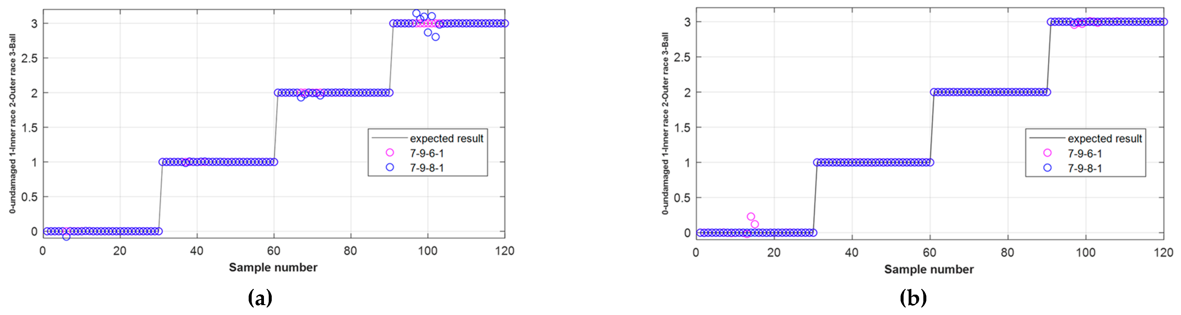
6.1. Fault Detector Based on MLP Network

Neural detectors based on MLP were tested first. The effectiveness of the detectors was checked in terms of the number of hidden layers (only for the fault detector, because in the case of the fault classifier the structure with one hidden layer was insufficient), the number of neurons in the hidden layer, the type of activation function, and the learning method. The research was conducted in the MATLAB environment, for the training and testing data sets given in Table 2. A schematic diagram of an example structure with two hidden layers is shown in Figure 8, with the input vector containing samples from either the FFT analysis or the ENV analysis.
The study of perceptron effectiveness due to the random nature of the initialization of the weights was carried out in 15 training and testing series. Table 3 shows the average percentage effectiveness of the fault detectors (type I) using the damage symptoms from the FFT analysis or from the ENV analysis, respectively, as mean values obtained after 15 series of NN testing. First, the tests were performed for two types of activation functions: tansig and logsig for various MLP structures using the Levenberg–Marquardt training method (trainlm) with the learning rate η = 0.5.
The use of the logsig activation function has a positive effect not only on the effectiveness of the detector operation, but also on the increase in the stability of the learning process in relation to the tansig function, both in the case of using ENV or the FFT itself. For all tested cases, the network achieved 100% efficiency. Next, the influence of the Levenberg–Marquardt method with Bayes regularization (trainbr learning) was checked, with weight limitation introduced. Tests were performed using the tansig activation function.
In the case of the 0–1 detector, after obtaining the proper structure, there are no significant differences between the use of ENV or the FFT itself. The differences are only noticeable during the learning process. The use of the Hilbert transform eliminates significant deviations from the expected values and ensures more repeatable network responses for individual learning and testing cycles, which significantly simplifies this process.
Then, the fault classifier (detector type II) was tested, whose task was to determine the type of bearing damage. Efficiency tests were performed analogously with FFT or ENV in 15 series of learning and testing. The results for variable parameters of MLPs and learning methods are presented in Table 4. The effectiveness of the MLP-based fault classifier was checked for various activation functions: tansig and logsig using the trainlm or trainbr learning methods and the learning rate η = 0.5.
Based on Table 4, it can be concluded that the use of the Hilbert transform improves the detection efficiency, with the structure reduced by two neurons in the hidden layers. The differences in the operation of the network based on FFT or ENV are noticeable in the results presented in Table 4, but not to the same extent as in the course of the exact output values of the analysed detectors, which are demonstrated in Figure 9. The output of the ENV-based detector fluctuates much less, regarding the expected value, than the output of the detector based on the FFT analysis. This greatly increases the stability and average accuracy of the detection.
In the case of the fault classifier, the study was carried out only for structures with two hidden layers, because the structure with one hidden layer was insufficient for the investigated problem and network responses were significantly different from the expected values.

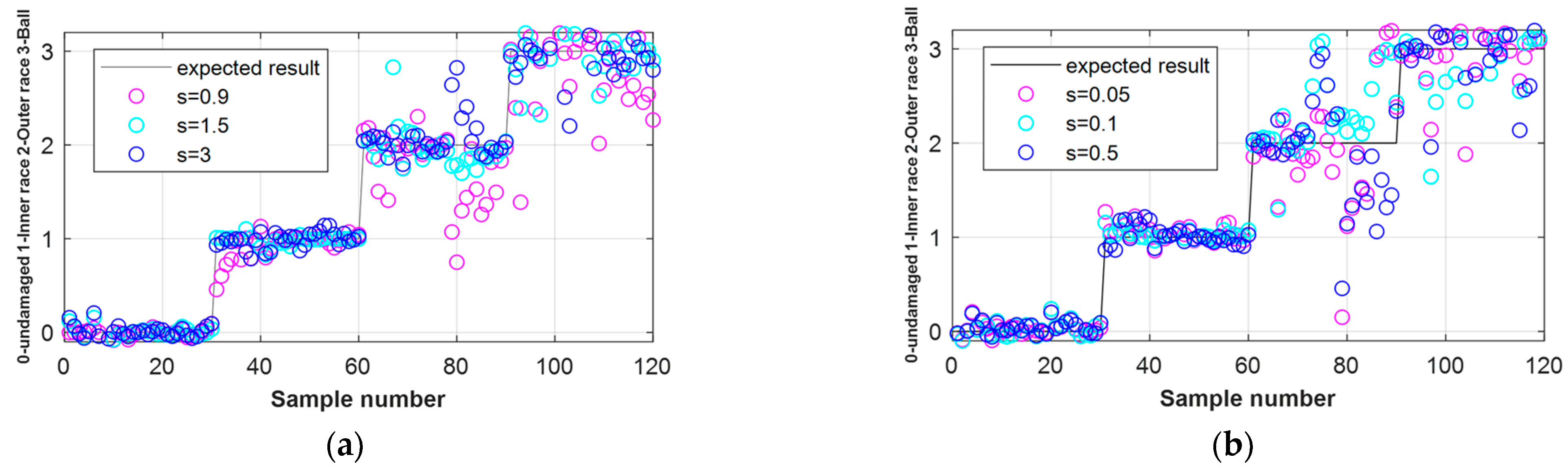
6.2. Fault Detector Based on RBF Network

RBF networks, unlike MLP, are characterized by the repeatability of results in the learning process. For the same network parameters, the same output results are always obtained, which significantly facilitates network training in the MATLAB environment, performed with the use of data sets presented in Table 1. The general structure of the studied networks with inputs created with FFT or ENV analyses, respectively, is shown in Figure 10.
First, tests were carried out for the damage detector and fault classifiers for different values of a spread parameter σ of the radial function and for a different number of radial neurons in the hidden layer, which was selected during the learning process. The respective results for both RBF-based detectors, with input vectors created using FFT or ENV analyses are collected in Table 5.
The use of ENV in the case of RBF network training data resulted in the correct operation of the network for a greater number of spread parameter values, σ. It made the selection of this parameter much easier in the process of detectors’ learning. Based on Table 5, it can be seen that with the increase in the value of the parameter σ, the effectiveness of NN using the data from the FFT analysis increases, and from the value of 0.3 it begins to decrease. In the case of fault detector based on ENV data, increasing the value of the spread parameter up to several times the value presented for FFT-based detector did not decrease its effectiveness.
In the case of the fault classifier, the RBF network also worked correctly for a larger set of the spread parameter after applying ENV, but not as large as in the case of the type I detector. On the exact output waveforms, presented in Figure 11, it can be observed that the RBF network response fluctuates strongly from the expected value, even when an ENV-based input vector is used. Nevertheless, with proper selection of parameters, 100% efficiency is possible.
The effectiveness of the RBF-based fault detectors was also tested in terms of the effect of limiting the number of neurons in the hidden layer. The analysis showed that the lack of constraints does not always ensure a better network efficiency. In the case of fault classifiers, too many neurons reduce the effectiveness. The network over-adjusts to the input data and the problem becomes oversized (Figure 12). In the case of network using only FFT data, the effectiveness drops to approximately 70%. The optimal value for all studied cases is about 100 neurons in the hidden layer.

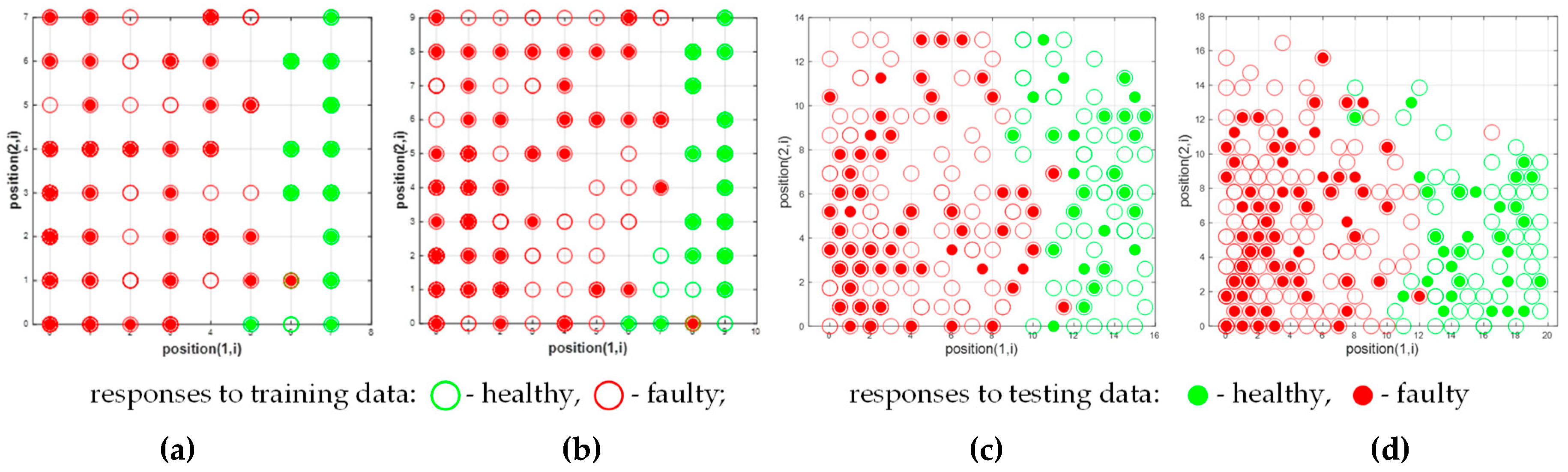
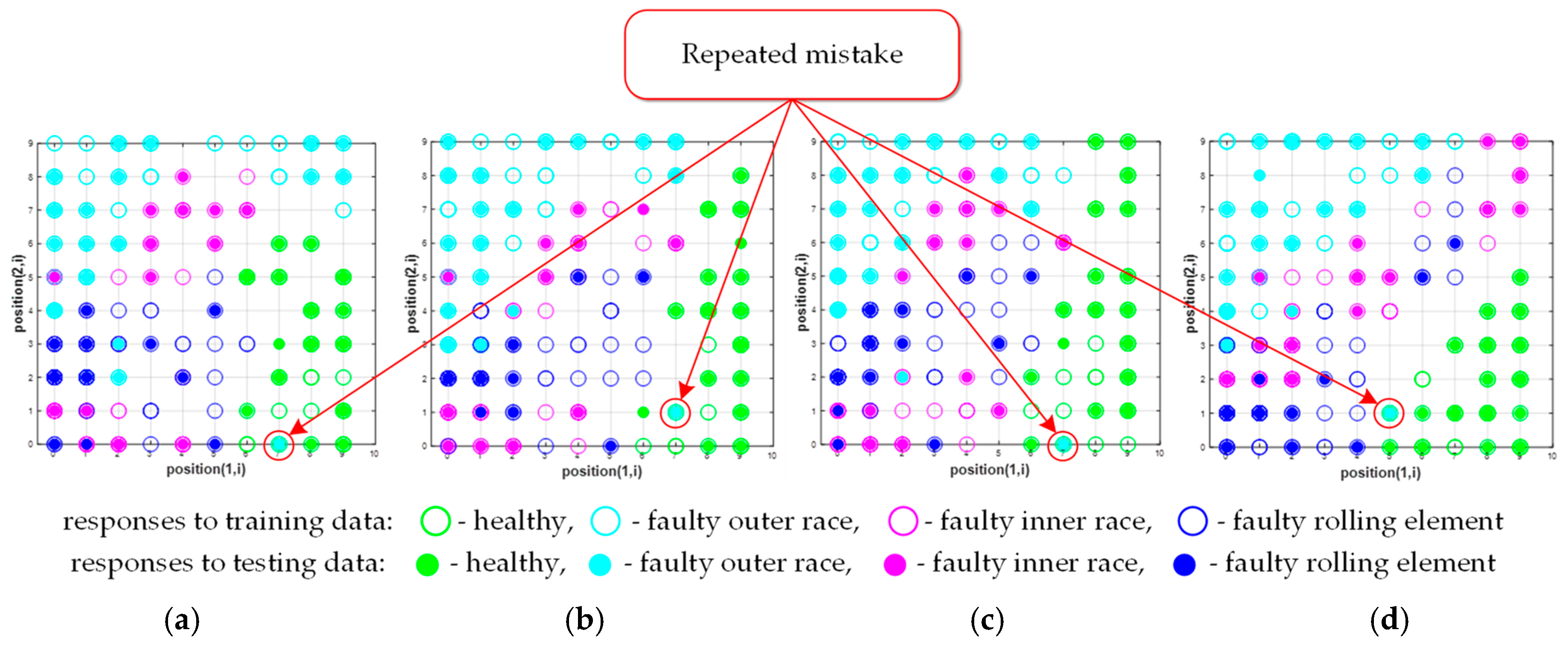
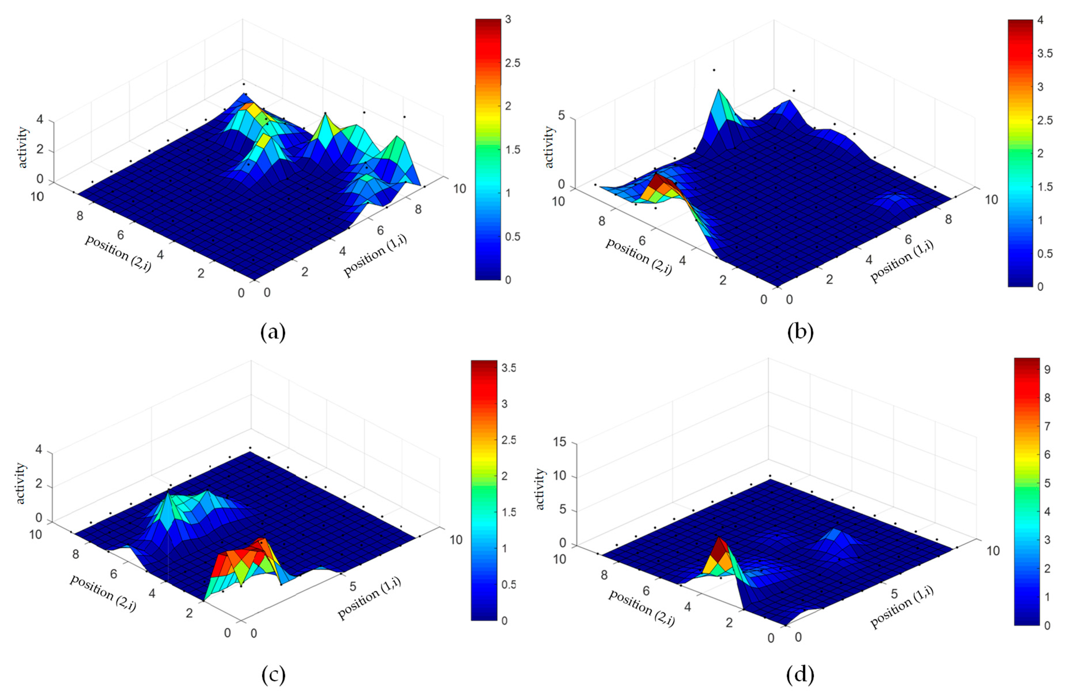
6.3. Fault Detector Based on SOM Network

Due to the sensitivity of Kohonen maps to the training data, only the network, whose inputs were harmonics obtained as a result of ENV analysis, was tested, for the same number of training and testing samples as before. The general schematic diagram of the structure is shown in Figure 13.
Tests were performed for different map sizes, neighbourhood radius, and distance functions. The research was carried out for a hexagonal grid, for neighbourhood radius equal to: 2 and 6, respectively, and for the distance function determined on the basis of the Euclidean distance (dist) and Link distance function (linkdist). The influence of the distance function and neighbourhood radius is presented in Figure 14, while results for variable size of SOM is shown in Figure 15. Testing Kohonen maps consisted of generating a map from the training data and then superimposing the results for the testing data on it. Overlapping of the respective areas indicated correct fault detection.
The neighbourhood radius equal to 2 and the Euclidean distance function dist allowed for a better separation of the areas on the map (Figure 14d) compared to the radius value equal to 6 and the function linkdist (Figure 14a). As shown in Figure 15c,d, error-free detection was obtained only for maps with increased sizes (16 × 16, 20 × 20). Based on the results presented in Figure 14 and Figure 15, the average effectiveness of SOM-based detectors was calculated, and the results are presented in Table 6 for different SOM structures and in Table 7 for hexagonal 10 × 10 map with different training parameters. It can be noticed that, even for a relatively small structure, the average effectiveness of the tested SOM-based detector is very high, over 98%.
SOM nets were also tested for the activity of individual areas on samples for healthy and damaged bearings (Figure 16). These areas are consistent with the maps shown in Figure 14 and Figure 15. Responses to samples from a damaged bearing cover a much larger area on the map, which is also visible in Figure 14 and Figure 15. Additionally, this area shows a much greater activity of neurons.
When the type of damage is classified, tangles appear on the map. It can be seen that the greatest relationship is between the failure of the rolling element and the inner race. These effects are shown in following figures. In the detectors based on the MLP and RBF networks, errors also appeared when distinguishing these specific failures.
As shown in Figure 17, irrespective of the value of the neighbourhood radius and the selected distance function, there is one, constantly repeating error on the maps. The mistake appeared when testing the information obtained for a bearing with a damaged outer race. In the case of the fault classifier, even increasing the number of neurons did not allow achieving 100% effectiveness (Figure 18). It was observed that, for each examined parameter, the error in the activity of the neuron of the healthy area was repeated due to damage to the outer raceway. Moreover, for fault detector (type I) the error appeared in a similar area. For many of the cases studied, this was the only wrong answer of the network.
Based on the results presented in Figure 17 and Figure 18, the average effectiveness of SOM-based classifiers was calculated and the results are presented in Table 8 for different SOM structures and in Table 9 for hexagonal 10 × 10 map with different training parameters. It can be noticed, that even for relatively small structure the average effectiveness of the tested SOM-based classifiers is also high, over 92%.
The activity of individual areas of the Kohonen map in response to single fault samples was also examined (Figure 19). Neurons respond least intensively to damage to the rolling element. Therefore, in each case, tangles appeared for this failure. In the case of other types of networks, errors also occurred most frequently for this fault type. It can also be seen that the areas of activity related to the failure of the rolling element and the outer raceway overlap to some extent, hence, the errors that occur when distinguishing them.
In the case of Kohonen maps, a graphical network response to both detector types is shown. The presented maps should be subject to additional analysis. The use of an additional classifier (e.g., cascaded MLP as in Reference [47]) analysing the obtained maps would automate the process of determining the type of the damage.

7. Summary and Conclusions

The application of classical NNs in the diagnostics of rolling bearings of a synchronous motor with permanent magnets enables the automation of this process and very high efficiency with a correctly selected structure and method of network training. This tool requires neither a mathematical model nor the involvement of a human expert in the diagnostic process, which are its significant advantages.
The use of the MLP network to develop the fault detector (type I) allowed for very high efficiency. For several structures, after 15 series of training and testing, it was possible to achieve 100% correct answers. In the case of the fault classifier (type II), achieving 100% efficiency required a more complex structure. One hidden layer was insufficient for the problem studied. The best results for both types of detectors were provided by the Levenberg–Marquardt learning method with Bayesian regularization and Log-sigmoid activation function. The classical MLP network provided the best efficiency and the smallest deviations from the expected value from all of the examined structures, especially for training data obtained from the analysis of the vibration acceleration signal using the Hilbert transformation.
Networks with radial basis functions are characterized by repeatability of responses for structures with the same parameters and the same input vector for each subsequent learning process. This is due to the fact that the initial weights are selected based on the input vector, and not randomly as in MLP networks. For this reason, the selection of RBF network parameters is less time-consuming.
The use of Kohonen maps does not fully automate the diagnostic process. In this case, it is necessary to use the evaluation of a human operator or add an algorithm that will be responsible for additional analysis of the result obtained by SOM. Nevertheless, Kohonen maps seem to be the most interesting for further research of all of the structures tested. The k-means algorithm is most often used to automate the result classification process [48,49]. Kohonen network outputs may also be inputs for other networks, which will ensure full automation of the process, as proposed in Reference [47]. For such purposes, studies can be carried out with both MLP and RBF networks. An important advantage of using Kohonen maps is the lack of difficulties in selecting their parameters.
The industry requires solutions that ensure an efficient and automated diagnostic process. The proposed NNs can be easily implemented using a low-budget integrated hardware platform based on, e.g., Arm Cortex-M or similar processors, or the diagnostics can be based on the measurement infrastructure existing in the industry and its extension with additional neural detectors. An exemplary concept of a cheap diagnostic system is presented in [14]. Based on the presented work, it can be concluded that classical NNs still are able to meet these requirements and are much less time-consuming in training and simpler in practical implementation than more popular deep-learning networks.

Author Contributions

All authors contributed equally to the concept of the paper, and proposed the methodology, formal analyses, and validation, P.E., K.J., and T.O.-K.; software, P.E. and K.J.; investigation, P.E. and K.J.; data curation, P.E. and K.J.; writing—original draft preparation, P.E. and K.J.; writing—review and editing, P.E., K.J., and T.O.-K.; visualization, P.E. and K.J.; supervision, T.O.-K.; project administration, T.O.-K.; funding acquisition, T.O.-K. All authors have read and agreed to the published version of the manuscript.

Funding

This research was supported by the National Science Centre Poland under grant number 2017/27/B/ST7/00816.

Conflicts of Interest

The authors declare no conflict of interest.

References

  1. Ullah, Z.; Lodhi, B.A.; Hur, J. Detection and Identification of Demagnetization and Bearing Faults in PMSM Using Transfer Learning-Based VGG. Energies 2020, 13, 3834. [Google Scholar] [CrossRef]
  2. Chen, Y.; Liang, S.; Li, W.; Liang, H.; Wang, C. Faults and Diagnosis Methods of Permanent Magnet Synchronous Motors: A Review. Appl. Sci. 2019, 9, 2116. [Google Scholar] [CrossRef] [Green Version]
  3. Rosero, J.; Romeral, L.; Rosero, E.; Urresty, J. Fault Detection in dynamic conditions by means of Discrete Wavelet Decomposition for PMSM running under Bearing Damage. In Proceedings of the 2009 Twenty-Fourth Annual IEEE Applied Power Electronics Conference and Exposition, Washington, DC, USA, 15–19 February 2009; pp. 951–956. [Google Scholar] [CrossRef] [Green Version]
  4. He, J.; Somogyi, C.; Strandt, A.; Demerdash, N.A.O. Diagnosis of stator winding short-circuit faults in an interior permanent magnet synchronous machine. In Proceedings of the 2014 IEEE Energy Conversion Congress and Exposition (ECCE), Pittsburgh, PA, USA, 14–18 September 2014; pp. 3125–3130. [Google Scholar] [CrossRef]
  5. Nkuna, J.S.R. Vibration Condition Monitoring and Fault Classification of Rolling Element Bearings Utilising Kohonen’s Self-organising Maps. Theses and Dissertations (Mechanical Engineering). Ph.D. Thesis, Vaal University of Technology, Vanderbijlpark, South Africa, 2013. [Google Scholar]
  6. Picot, A.; Obeid, Z.; Régnier, J.; Poignant, S.; Darnis, O.; Maussion, P. Statistic-based spectral indicator for bearing fault detection in permanent-magnet synchronous machines using the stator current. Mech. Syst. Signal Process. 2014, 46, 424–441. [Google Scholar] [CrossRef] [Green Version]
  7. Ye, M.; Huang, J. Bearing Fault Diagnosis under Time-Varying Speed and Load Conditions via Speed Sensorless Algorithm and Angular Resample. In Proceedings of the 2018 XIII International Conference on Electrical Machines (ICEM), Alexandroupoli, Greece, 3–6 September 2018; pp. 1775–1781. [Google Scholar] [CrossRef]
  8. Lu, S.; He, Q.; Zhao, J. Bearing fault diagnosis of a permanent magnet synchronous motor via a fast and online order analysis method in an embedded system. Mech. Syst. Signal Process. 2018, 113, 36–49. [Google Scholar] [CrossRef]
  9. Nembhard, A.D.; Sinha, J.K.; Pinkerton, A.J.; Elbhbah, K. Fault diagnosis of rotating machines using vibration and bearing temperature measurements. Diagnostyka 2013, 14, 45–51. [Google Scholar]
  10. Rosero, J.; Cusido, J.; Ortega, J.A.; Romeral, L.; Garcia, A. PMSM Bearing Fault Detection by means of Fourier and Wavelet transform. In Proceedings of the IECON 2007—33rd Annual Conference of the IEEE Industrial Electronics Society, Taipei, Taiwan, 5–8 November 2007; pp. 1163–1168. [Google Scholar] [CrossRef]
  11. Liu, H.; Li, D.; Yuan, Y.; Zhang, S.; Zhao, H.; Deng, W. Fault Diagnosis for a Bearing Rolling Element Using Improved VMD and HT. Appl. Sci. 2019, 9, 1439. [Google Scholar] [CrossRef] [Green Version]
  12. Ren, B.; Yang, M.; Chai, N.; Li, Y.; Xu, D. Fault Diagnosis of Motor Bearing Based on Speed Signal Kurtosis Spectrum Analysis. In Proceedings of the 2019 22nd International Conference on Electrical Machines and Systems (ICEMS), Harbin, China, 11–14 August 2019; pp. 1–6. [Google Scholar] [CrossRef]
  13. Skora, M.; Ewert, P.; Kowalski, C.T. Selected Rolling Bearing Fault Diagnostic Methods in Wheel Embedded Permanent Magnet Brushless Direct Current Motors. Energies 2019, 12, 4212. [Google Scholar] [CrossRef] [Green Version]
  14. Ewert, P.; Kowalski, C.T.; Orlowska-Kowalska, T. Low-Cost Monitoring and Diagnosis System for Rolling Bearing Faults of the Induction Motor Based on Neural Network Approach. Electronics 2020, 9, 1334. [Google Scholar] [CrossRef]
  15. Senanayaka, J.S.L.; Huynh, V.K.; Robbersmyr, K.G. A robust method for detection and classification of permanent magnet synchronous motor faults: Deep autoencoders and data fusion approach. J. Phys. Conf. Ser. 2018, 1037, 032029. [Google Scholar] [CrossRef]
  16. Senanayaka, J.S.L.; Huynh, V.K.; Robbersmyr, K.G. Fault detection and classification of permanent magnet synchronous motor in variable load and speed conditions using order tracking and machine learning. J. Phys. Conf. Ser. 2018, 1037, 032028. [Google Scholar] [CrossRef]
  17. Akar, M.; Hekim, M.; Orhan, U. Mechanical fault detection in permanent magnet synchronous motors using equal width discretization-based probability distribution and a neural network model. Turk. J. Electr. Eng. Comput. Sci. 2015, 23, 813–823. [Google Scholar] [CrossRef]
  18. Pandarakone, S.E.; Mizuno, Y.; Nakamura, H. Distinct Fault Analysis of Induction Motor Bearing Using Frequency Spectrum Determination and Support Vector Machine. IEEE Trans. Ind. Appl. 2017, 53, 3049–3056. [Google Scholar] [CrossRef]
  19. Navasari, E.; Asfani, D.A.; Negara, M.Y. Detection Of Induction Motor Bearing Damage With Starting Current Analysis Using Wavelet Discrete Transform And Artificial Neural Network. In Proceedings of the 2018 10th International Conference on Information Technology and Electrical Engineering (ICITEE), Kuta, Indonesia, 24–26 July 2018; pp. 316–319. [Google Scholar] [CrossRef]
  20. Hoang, D.T.; Kang, H.J. A Motor Current Signal-Based Bearing Fault Diagnosis Using Deep Learning and Information Fusion. IEEE Trans. Instrum. Meas. 2020, 69, 3325–3333. [Google Scholar] [CrossRef]
  21. Zhou, J.; Qin, Y.; Kou, L.; Yuwono, M.; SU, S. Fault detection of rolling bearing based on FFT and classification. J. Adv. Mech. Des. Syst. Manuf. 2015, 9. [Google Scholar] [CrossRef] [Green Version]
  22. Li, B.; Chow, M.-Y.; Tipsuwan, Y.; Hung, J.C. Neural-Network-Based Motor Rolling Bearing Fault Diagnosis. IEEE Trans. Ind. Electron. 2000, 47, 1060–1069. [Google Scholar] [CrossRef] [Green Version]
  23. Haroun, S.; Nait Seghir, A.; Touati, S. Feature Selection for Enhancement of Bearing Fault Detection and Diagnosis Based on Self-Organizing Map. In Recent Advances in Electrical Engineering and Control Applications; Chadli, M., Bououden, S., Zelinka, I., Eds.; Lecture Notes in Electrical Engineering; Springer: Cham, Switzerland, 2017; Volume 411. [Google Scholar] [CrossRef]
  24. Tandon, N.; Choudhury, A. A review of vibration and acoustic measurement methods for the detection of defects in rolling element bearings. Tribol. Int. 1999, 32, 469–480. [Google Scholar] [CrossRef]
  25. Zandi, O.; Poshtan, J. Brushless DC Motor Bearing Fault Detection Using Hall Effect Sensors and a Two-Stage Wavelet Transform. In Proceedings of the 26th Iranian Conference on Electrical Engineering (ICEE2018), Mashhad, Iran, 8–10 May 2018; pp. 827–833. [Google Scholar] [CrossRef]
  26. Liu, Z.; Zhang, L. A review of failure modes, condition monitoring and fault diagnosis methods for large-scale wind turbine bearings. Measurement 2020, 149, 107002. [Google Scholar] [CrossRef]
  27. Rolling Bearings—Damage and Failures—Terms, Characteristics and Causes; International Organization for Standardization: Geneva, Switzerland, 2017; ISO 15243:2017; Publication date: March 2017.
  28. Radu, C. The Most Common Causes of Bearing Failure and the Importance of Bearing Lubrication. RKB Technical Review. February 2010, pp. 1–7. Available online: https://www.rkbbearings.com/en/publications.php#sec12 (accessed on 23 December 2020).
  29. Bearing Damage and Failure Analysis, SKF Group, PUB BU/I3 14219/2 EN. June 2017, pp. 1–106. Available online: https://www.skf.com/binaries/pub12/Images/0901d1968064c148-Bearing-failures---14219_2-EN_tcm_12-297619.pdf (accessed on 23 December 2020).
  30. Smith, S.W. Digital Signal Processing: A Practical Guide for Engineers and Scientists; Elsevier Science: Burlington, VT, USA, 2002. [Google Scholar] [CrossRef]
  31. Lee, C.-Y.; Hsieh, Y.-H. Bearing damage detection of BLDC motors based on current envelope analysis. Meas. Sci. Rev. 2012, 12, 290–295. [Google Scholar] [CrossRef] [Green Version]
  32. Espinosa, A.G.; Rosero, J.A.; Cusid’o, J.; Romeral, L.; Ortega, J.A. Fault Detection by Means of Hilbert–Huang Transform of the Stator Current in a PMSM With Demagnetization. IEEE Trans. Energy Convers. 2010, 25, 312–318. [Google Scholar] [CrossRef] [Green Version]
  33. Bishop, M.C. Neural Networks for Pattern Recognition, 1st ed.; Oxford University Press: New York, NY, USA, 1996. [Google Scholar]
  34. Haykin, S. Neural Networks, a Comprehensive Foundation; Macmillan College Publishing Company: New York, NY, USA, 1994. [Google Scholar]
  35. Yu, H.; Wilamowski, B.M. Levenberg–Marquardt Training. In Industrial Electronics Handbook, 2nd ed.; Chapter 12; Intelligent Systems, CRC Press: Boca Raton, FL, USA, 2011; Volume 5, pp. 12-1–12-15. [Google Scholar]
  36. Demuth, H.; Beale, M. Neural Network Toolbox—User’s Guide; Version 4; The MathWorks, Inc.: Natick, MA, USA, 2004. [Google Scholar]
  37. Du, Y.-C.; Stephanus, A. Levenberg-Marquardt Neural Network Algorithm for Degree of Arteriovenous Fistula Stenosis Classification Using a Dual Optical Photoplethysmography Sensor. Sensors 2018, 18, 2322. [Google Scholar] [CrossRef] [Green Version]
  38. Zayani, R.; Bouallegue, R.; Roviras, D. Levenberg-Marquardt learning neural network for adaptive predistortion for time-varying HPA with memory in OFDM systems. In Proceedings of the EUSIPCO2008—16th European Signal Processing Conference, Lausanne, Switzerland, 25–29 August 2008; pp. 1–6. Available online: https://hal.archives-ouvertes.fr/hal-02457894 (accessed on 9 December 2020).
  39. Jazayeri, K.; Jazayeri, M.; Uysal, S. Comparative Analysis of Levenberg-Marquardt and Bayesian Regularization Backpropagation Algorithms in Photovoltaic Power Estimation Using Artificial Neural Network. In Advances in Data Mining. Applications and Theoretical Aspects. ICDM 2016; Perner, P., Ed.; Lecture Notes in Computer Science; Springer: Cham, Switzerland, 2016; Volume 9728. [Google Scholar] [CrossRef]
  40. Suliman, A.; Omarov, B.S. Applying Bayesian Regularization for Acceleration of Levenberg-Marquardt based Neural Network Training. Int. J. Interact. Multimed. Artif. Intell. 2018, 5, 68–72. [Google Scholar] [CrossRef]
  41. Gil, D.; Johnsson, M. Supervised SOM Based Architecture versus Multilayer Perceptron and RBF Networks. In Proceedings of the 26th Annual Workshop of the Swedish Artificial Intelligence Society (SAIS), Uppsala, Sweden, 20–21 May 2010; pp. 15–24. [Google Scholar]
  42. Bayram, S.; Ocal, M.E.; Laptali Oral, E.; Atis, C.D. Comparison of multilayer perceptron (MLP) and radial basis function (RBF) for construction cost estimation: The case of Turkey. J. Civ. Eng. Manag. 2016, 22, 480–490. [Google Scholar] [CrossRef] [Green Version]
  43. Fath, A.H.; Madanifar, F.; Abbasi, M. Implementation of multilayer perceptron (MLP) and radial basis function(RBF) neural networks to predict solution gas-oil ratio of crude oil systems. Petroleum 2020, 6, 80–91. [Google Scholar] [CrossRef]
  44. Jaganathan, B.; Venkatesh, S.; Bhardwaj, Y.; Sridhar, V. Optimal parameters estimation of a BLDC motor by Kohonen’s Self Organizing Map Method. In Proceedings of the 2011 IEEE Recent Advances in Intelligent Computational Systems, Trivandrum, Kerala, India, 22–24 September 2011; pp. 068–071. [Google Scholar] [CrossRef]
  45. Jacobs, S.; Rios-Gutierrez, F. Self-organizing maps for monitoring parameter deterioration of DC and AC motors. In Proceedings of the 2013 Proceedings of IEEE Southeastcon, Jacksonville, FL, USA, 4–7 April 2013; pp. 1–6. [Google Scholar] [CrossRef] [Green Version]
  46. Khalfaoui, N.; Salhi, M.S.; Amiri, H. The SOM tool in mechanical fault detection over an electric asynchronous drive. In Proceedings of the 2016 4th International Conference on Control Engineering & Information Technology (CEIT), Hammamet, Tunisia, 16–18 December 2016; pp. 1–6. [Google Scholar] [CrossRef]
  47. Skowron, M.; Orlowska-Kowalska, T. Efficiency of cascade-connected neural networks in detecting initial faults to induction motor drive electric windings. Electronics 2020, 9, 1314. [Google Scholar] [CrossRef]
  48. Dogan, Y.; Birant, D.; Kut, A. SOM++: Integration of Self-Organizing Map and K-Means++ Algorithms. In Machine Learning and Data Mining in Pattern Recognition. MLDM 2013; Perner, P., Ed.; Lecture Notes in Computer Science; Springer: Berlin/Heidelberg, Germany, 2013; Volume 7988. [Google Scholar] [CrossRef]
  49. Bataineh, A.K.; Samkari, M.H.; Abdualla, A.; Al-Azzam, S. K-Means Clustering in WSN with Kohonen SOM and Conscience Function. Mod. Appl. Sci. 2019, 13, 63–75. [Google Scholar] [CrossRef]
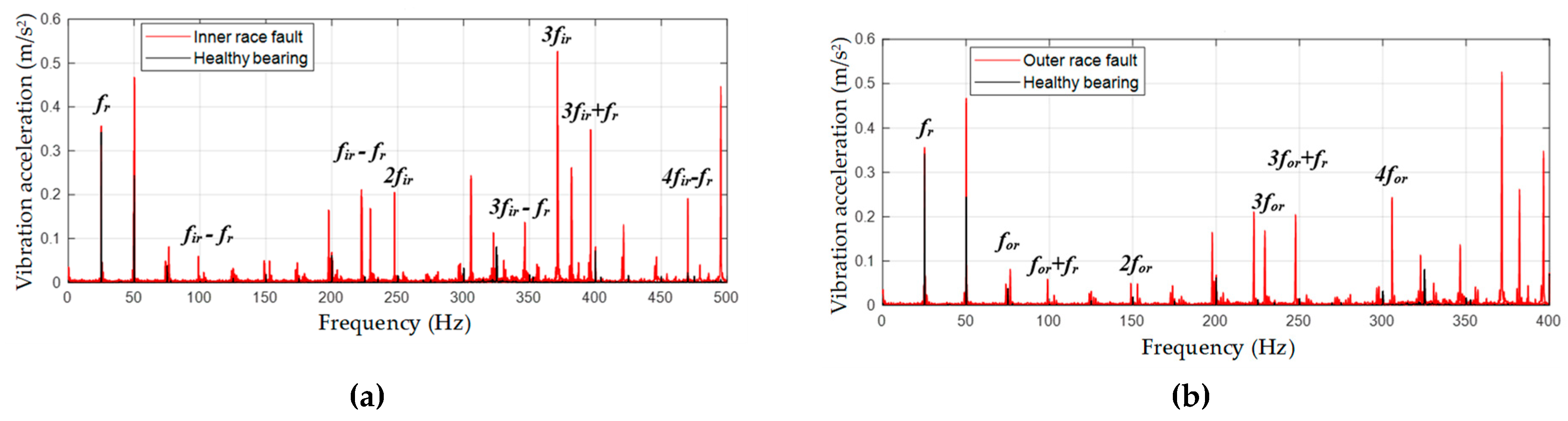
Figure 1. Diagram of the construction of a rolling bearing.
Energies 14 00712 g001
Figure 2. Example of structure of the feedforward multilayer perceptron (MLP) network.
Energies 14 00712 g002
Figure 3. General structures of radial basis function (RBF) network.
Energies 14 00712 g003
Figure 4. General architecture of Kohonen map.
Energies 14 00712 g004
Figure 5. Schematic diagram and photo of the laboratory stand.
Energies 14 00712 g005
Figure 6. Examples of vibration spectra for damage to the inner (a) and outer (b) raceways for the supply frequency fs = 100 Hz of the permanent magnet synchronous motor (PMSM) drive.
Energies 14 00712 g006
Figure 7. Examples of harmonic amplitudes with characteristic frequencies obtained using envelope (ENV) for vibration acceleration signal; different load torques and supplying frequencies of PMSM drive.
Energies 14 00712 g007
Figure 8. Schematic diagram of a fault detector or fault classifier based on MLP network with different input signals: after FFT or ENV analysis.
Energies 14 00712 g008
Figure 9. Waveforms of output values from the MLP-based fault classifier (type II) using the tansig activation function, trainlm learning method, learning rate η = 0.5 for various MLP structures based on the ENV (a) or FFT (b) analyses.
Energies 14 00712 g009
Figure 10. Schematic diagram of a fault detector or fault classifier based on RBF network with different input signals: after FFT or ENV analysis.
Energies 14 00712 g010
Figure 11. Waveforms of output values from the fault classifier (type II) for different spread values of RBF network based on input vectors from ENV (a) or FFT (b) analyses.
Energies 14 00712 g011
Figure 12. Influence of the number of radial neurons in the hidden layer on the effectiveness of the RBF-based fault detector for different spread values and input from FFT analysis and σ = 0.1 (a), σ = 0.5 (b), ENV analysis and σ = 0.9 (c), σ = 3 (d).
Energies 14 00712 g012
Figure 13. General schematic diagram of the self-organizing map (SOM).
Energies 14 00712 g013
Figure 14. Results of the SOM-based fault detector for the 10 × 10 hexagonal map and the linkdist distance function for different values of the neighbourhood radius: 2 (a), 6 (b), and for different distance function: linkdist (c), dist (d) with the neighbourhood radius equal to 2.
Energies 14 00712 g014
Figure 15. Results of the SOM-based fault detector for various sizes of the hexagonal map 8 × 8 (a), 10 × 10 (b), 16 × 16 (c), 20 × 20 (d) with the neighbourhood radius equal 2 and the linkdist function.
Energies 14 00712 g015
Figure 16. Active areas of the 10 × 10 Kohonen map in the case of an undamaged bearing (a) and with a fault (b) for the neighbourhood radius equal to 2 and the linkdist function.
Energies 14 00712 g016
Figure 17. The results of the SOM classifier for the 10 × 10 hexagonal map and the linkdist distance function for different values of the neighbourhood radius: 2 (a), 6 (b), and for different distance function: linkdist (c), dist (d) with the neighbourhood radius equal to 2.
Energies 14 00712 g017
Figure 18. The results of the SOM-based classifier for different sizes of the hexagonal map: 8 × 8 (a), 10 × 10 (b), 16 × 16 (c), 20 × 20 (d) with the neighbourhood radius equal to 2 and the linkdist distance function.
Energies 14 00712 g018
Figure 19. Active areas of 10 × 10 SOM map in the case of healthy bearing (a), damage to outer raceway (b), inner raceway (c), rolling element (d) for the neighbourhood radius equal to 2 and the linkdist distance function.
Energies 14 00712 g019
Table 1. Examples of frequency values for damage harmonics.
fs (Hz)fr (Hz)3fir (Hz)4fir (Hz)2for (Hz)3for (Hz)4fre + fr (Hz)
20574.259930.545.7584.8
6015222.7529791.5137.25254.4
10025371.25495152.5228.75424
Table 2. The structure of the training and testing data with the division into the fast Fourier transform (FFT) and envelope analysis (ENV) of the vibration signal.
Number of Samples FFT AnalysisENV Analysis
Training set240240
Testing set120120
Table 3. Comparison of the effectiveness of the fault detectors of type I (0–1 detectors).
StructureFFTENV
7-4-17-5-4-17-4-17-5-4-1
tansig + trainlm98.33%100%95%100%
logsig + trainlm100%100%100%100%
tansig + trainbr100%100%100%100%
Table 4. Comparison of the effectiveness of fault classifiers (detectors type II) determining the type of damage.
StructureFFTENV
7-9-6-17-9-8-17-9-6-17-9-8-1
tansig + trainlm98.94%99.22%99.61%99.50%
logsig + trainlm99.17%97.2%99.17%100%
tansig + trainbr99.5%97.2%99.94%99.83%
Table 5. RBF network efficiency for fault detector and classifier using FFT or ENV analyses for different spread, σ, coefficients.
Detector
Type
σ0.050.090.10.30.50.91.21.523
Fault detector
(type I)
FFT92.5%95%95%100%95%
ENV 96.7%100%100%100%100%
Fault classifier
(type II)
FFT92.5%97.5%96.7%95.8%90%
ENV 85%90%98.3%100%98.3%
Table 6. Comparison of the effectiveness of the SOM-based fault detector with the neighbourhood radius equal 2 and the linkdist function for various sizes of the hexagonal map.
ParametersSizes of the Hexagonal Map
8 × 810 × 1016 × 1620 × 20
Average effectiveness98.7%98.8%99.3%99%
Table 7. Comparison of the effectiveness of the SOM-based fault detector for the 10 × 10 hexagonal map and the linkdist distance function for different values of the neighbourhood radius and for different distance function with the neighbourhood radius equal to 2.
ParametersNeighbourhood RadiusDistance Function
26linkdistdist
Average effectiveness98.6%98.7%98.7%98.8%
Table 8. Comparison of the effectiveness of the SOM-based classifier with the neighbourhood radius equal 2 and the linkdist function for various sizes of the hexagonal map.
ParametersSizes of the Hexagonal Map
8 × 810 × 1016 × 1620 × 20
Average effectiveness83.3%92.3%95.3%95%
Table 9. Comparison of the effectiveness of the SOM-based classifier for the 10 × 10 hexagonal map and the linkdist distance function for different values of the neighbourhood radius, and for different distance function with the neighbourhood radius equal to 2.
ParametersNeighbourhood RadiusDistance Function
26linkdistdist
Average effectiveness92%92.3%90.8%92.5%
Publisher’s Note: MDPI stays neutral with regard to jurisdictional claims in published maps and institutional affiliations.

