Article

Corrosion Repair of Pipelines Using Modern Composite Materials Systems: A Numerical Performance Evaluation †

1
Department of Mechanical Engineering, Petroleum-Gas University of Ploiesti, 100680 Ploiesti, Romania
2
Department of Informatics, Information Technology, Mathematics and Physics, Petroleum-Gas University of Ploiesti, 100680 Ploiesti, Romania
*
Author to whom correspondence should be addressed.
This paper is an extended version of our paper published in 2019 ASME 38th International Conference on Ocean, Offshore & Arctic Engineering OMAE, Glasgow, Scotland, UK, 9–14 June 2019, Paper No. 96279.
Energies 2021, 14(3), 615; https://doi.org/10.3390/en14030615
Submission received: 23 December 2020 / Revised: 20 January 2021 / Accepted: 22 January 2021 / Published: 26 January 2021
(This article belongs to the Special Issue Drilling Technologies for the Next Generations)

Abstract

:
Pipe corrosion is a frequent phenomenon, and if repairs are delayed it could lead to environmental damage. Drilling activities can expand only when sufficient surface transportation capacity for the produced fluids exists and thus good maintenance of the transportation system is important. Furthermore, the technology presented herein can be easily upgraded as a repair solution for surface casing section below the casing head, which have been repeatedly reported as being highly corroded for older wells. This paper presents the results of the research work carried out by the authors in order to evaluate the design methods of the modern composite material systems used to repair steel pipes carrying hydrocarbons upon which local metal loss defects (generated by corrosion and/or erosion processes) have been detected. The pipe repair technologies consisting of the application of composite material wraps (made of a polymeric matrix and reinforcing fabric) are perceived as being advantageous alternative solutions for substituting the conventional technologies, which require welding operations to be performed in the corroded pipe areas. The performance and the design methods of the composite repair systems have been investigated by evaluating the reinforcement effects (the restoration level of the damaged pipe mechanical strength) generated by the applied composite wraps as a function of their geometry and mechanical properties. To that purpose, numerical models based on finite elements (previously developed by the authors and certified by comparing them with the results of several experimental programs performed within our university) have been used. The calculation methods proposed in literature (among which a method previously proposed by the authors) to define the composite wrap dimensions (thickness and length) for a given pipe have been compared to the numerical results in order to select the most adequate solution for the design of the composite repair system. The influence in the design process of the defect orientation and of its width has also been investigated.

1. Introduction

Steel pipes are frequently used in the transmission lines for hydrocarbons (crude oil, natural gas, liquid petroleum products etc.) or other fluids (water, ammonia etc.). They are also used in the transportation systems required by drilling activities. As these pipes provide significant services, the activities needed for their adequate maintenance and repair require special attention.
One of the most common factors affecting the integrity and strength of steel pipes used for hydrocarbons transportation is the corrosion process, causing damage of the pipe components by the chemical or electrochemical action of the transported fluid or of the environment in which the pipe is located. This phenomenon usually generates local imperfections or defects, of the metal loss type, on their inner and/or outer surfaces. A throughout characterization of such defects, including the methods used for their assessment (intended to define the necessity and opportunity of repairing the damaged areas of the steel pipes), can be found in [1].
The aggressiveness of both the circulating fluids and the soil in which the transmission pipelines are laid are important factors influencing their operating behavior. The corrosion processes (external, internal, hydrogen induced cracking or stress corrosion cracking) controlled by these factors represent hazards with high probability of occurrence and great potential to generate progressive degradation and cause failure of the steel pipes during their operation [2,3,4,5,6,7,8].
Methods for detecting imperfections or defects (including the corrosion generated one) in steel pipes are mainly based on the inspections using intelligent PIG systems, but also other systems known as NoPIG have begun to expand. Intelligent PIGs are complex electronic and mechanical devices used for direct inspection of the pipe, capable of providing information about imperfections and defects such as local metal loss or cracks-like in the pipe wall [9,10,11,12,13]. A frequently used NoPIG method is the “Guided Wave” method, which consists in the ultrasound movement guided by the geometry of the object in which they propagate. Details about this system can be found in [14,15,16,17,18,19].
Since the transmission process of various fluids is of great importance and therefore must be continuously provided, the technological procedures developed for steel pipe repair that can be applied without removing the pipelines from service are the ones presently preferred. Among these, the repair technologies consisting of the application of composite material wraps/sleeves are perceived as being advantageous alternative solutions to the conventional technologies, based on welding operations executed in the damaged areas (requiring special precautions if performed on operating pipes which carry fluids under pressure). A detailed description of the composite repair systems, including a comparison with other repair technologies, can be found in [20].
Furthermore, such repair technology can be easily upgraded to be used as an alternative repair solution for surface casing section below the casing head, which have been repeatedly reported as being highly corroded for older wells.
The composite repair technology can be efficiently used not only in the case of steel pipes with corrosion (metal loss) defects, but also for pipes with crack-like defects. The object of the present paper consists of the first type of defects mentioned above, previously analyzed by the authors in [21,22,23]. However, we intend to analyze in the future also the use of composite materials to repair crack-like defects, including their effect on crack propagation, investigated in [24,25]. Such analysis would require modeling fracture in steel pipes, for which efficient approaches are shown in [26,27].
In the following sections, after a short characterization of the composite repair systems developed for steel pipes, including the main mechanical properties of the composite materials commonly used, the modalities of assessing the performance of such repair systems are discussed, with reference to previous investigations performed by the authors [21], that have been extended in the present paper.
Due to the fact that the performance of any repair systems is significantly influenced by its proper design and materials selection, the methods used to that purpose for the composite systems were also investigated, including one previously developed by the authors, described in [22,23].
While our previous work from [22,23] has been dedicated to the comparison of the most relevant design methods presently used for the composite repair systems intended for corroded steel pipes, in this paper our investigations have been focused on assessing the most adequate analytical formulas to be used for the design of the composite wrap by comparing their results with the ones obtained using finite elements simulations to analyze the state of stress in the steel pipe after repair.
In order to select the most adequate method for the design of the composite wraps used for steel pipes repair, two relevant case studies have been analyzed using such simulations. The results and conclusions of these analyses, detailed in [21], are briefly described in this paper.
In addition to our previous investigations from [21,22,23], the effects in the composite repair design procedure of the defect circumferential extent (width), of its orientation with respect to the steel pipe axis and of the fillet radius used when machining the defect area (as required by the typical repair procedure) have been investigated and the results are discussed in the present paper.
All the investigations performed in the present paper, as well as in [21], have taken into account only the most relevant mechanical loading affecting transmission pipelines, i.e., the internal pressure. No additional loads or temperature variations have been considered in our analyses. This was due to the fact that the composite repair systems are most frequently used for gas transmission pipelines for which temperature variations or other supplementary loads are not relevant with the exception (only in some conditions) of axial loads. However, the authors plan to investigate the effect of additional axial loads and/or temperature variations in their future research work.

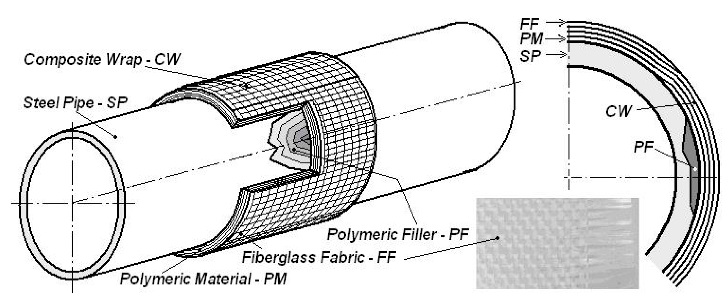
2. Characterization of the Composite Materials Repair Systems

A typical repair system using composite materials, intended for steel pipes repair, consists of the following elements [20,21,22]:
(1)
the substrate (pipe/pipe component to be repaired);
(2)
the procedure for the substrate surface preparation in the area to be repaired;
(3)
the polymeric filler, used to fill the defect area and thus to reconstruct the substrate configuration;
(4)
the repairing wrap made of a composite material and its components (polymeric resin matrix and reinforcing fibers or composite material layers bonded by a polymeric adhesive);
(5)
the repair procedure (application and quality verification procedures).
There are three types of composite repair systems presently in use for steel pipes [20,21,22]:
(1)
layered systems, obtained by wrapping a composite band/tape with the help of an adhesive;
(2)
wet lay-up systems of monolithic type, obtained by applying successive layers of polymeric resin and reinforcing fibers/fabric;
(3)
hybrid systems, using complex materials, by combining the components of the systems 1 and 2.
Figure 1 shows an example for a wet lay-up system using fiberglass fabric as arming material.
The achievement of a good quality pipe repair using a composite system presupposes a comprehensive knowledge of the mechanical properties of the composite material which behaves as an orthotropic plate [22,23]. The following such properties are required for the performance evaluation:
(1)
elastic constants: the tensile modulus in the circumferential direction, Ecc, and in the axial direction, Eac; the Poisson ratio in the circumferential direction, μc, and the shear modulus, Gc;
(2)
tensile strength, at least in the circumferential direction: short-term, Rmcc, and long-term, Rmclc;
(3)
elongation at break, at least in the circumferential direction, Acc.
Table 1 summarizes the main mechanical properties of five types of composite materials, most commonly used at present for steel pipes repair, obtained from their presentation documents (more details, including temperature influence, are included in [22,23]). It has to be mentioned that type V composite, as it is armed with carbon fibers, could generate additional corrosion processes in a steel pipe and is therefore less frequently used.
As the long-term values of the mechanical properties guaranteed for the composite materials is sometimes not provided by their manufacturers [22,23], we recommend to assess the value of the long-term mechanical strength in the circumferential direction using the equation:
Rmclc = f Rmcc,
where f is a service factor, accounting for the decrease in time of the mechanical strength, f = 0.50 … 0.67 [29]; in the followings, we have conservatively assumed that f = 0.50.
In addition to the properties in Table 1, the allowable (long-term) values for the stress/strain of the composite material should also be defined, at least for the circumferential direction (σaccacc). When assessing these values, the temperature influences upon the composite material properties should also be considered, as detailed in [22]. The assumed values (considering that no additional/supplementary loads will be applied to the steel pipe during its operation) for the types of composite materials included in Table 1, according to [22], are:
  • temperature derating factor (for all materials): ft = 0.977;
  • allowable strain for both directions (axial and circumferential) for type II composite: εacc = 0.0031;
  • allowable strain for both directions for the other four types of composite materials: εacc = 0.0024.
The different allowable strain value defined for the type II composite is due to the fact that this value depends on the Ecc/Eac ratio which is smaller than 2, while for the other composites: Ecc/Eac > 2.
The allowable stress value in the circumferential direction can be calculated as:
σacc = min (Ecc εacc; f Rmcc).

3. Reinforcement Effect Evaluation and Design of the Composite Material Repair Systems

In order to evaluate the performance of a given composite repair system, the reinforcement/consolidation effects generated by the applied composite wrap should be assessed. Such effect can be expressed by the restoration level of the pipe mechanical strength after its repair.
The stress-strain states in the corroded pipe area under the operational (internal) pressure, before and after repair, should be investigated and compared, together with the maximum stress/strain value in the pipe wall. Such investigations can be performed experimentally (results of pressure tests—some performed with the contribution of the authors—can be found in [28,30,31]), numerically (using finite elements simulation models—shown in [23,32,33]) or analytically.
In order to perform an assessment of the stress-strain state from a steel pipe wall, in which a local metal loss defect has been detected and which has been repaired using composite material wraps, the following data are required [22,23]:
(1)
Dimensional characteristics of the steel pipe: nominal outside diameter, De; nominal wall thickness, tn (for an accurate assessment, effective values from the damaged area are needed); the relative pipe thickness, trp, its internal radius, ap, and its external radius, bp, defined as follows:
t r p = t n D e ;   a p = D e 2 t n ;   b p = D e 2 .
(2)
Mechanical properties of the steel pipe to be repaired: Young modulus, Ep; yield strength, Ryp (usually expressed by the proof strength, total extension, Rt0.5p); tensile strength, Rmp; percentage elongation after fracture, Afp; Poisson ratio, μp; toughness properties.
(3)
Design conditions and the normal operating conditions of the repaired pipe: design pressure, pc; supplementary loads (not considered in the present paper); maximum and minimum operating temperatures. In addition, the allowable stress, σap, and the maximum allowable operating pressure, paopc, of the pipe should also be calculated, using the equations:
σ ap = f d   R yp ;   p a o = 2 t n · σ a p D e t n .
where fd is the design factor for the pipeline. In this paper, Location Class 1 has been considered in the calculation, corresponding to an assumed value of the pipeline design factor: fd = 0.72.
(4)
Characteristic dimensions of the metal loss defect detected in the steel pipe wall: maximum depth, dmax; axial/longitudinal extent, sp; circumferential extent, cp. Relative defect depth and length could also be calculated, using the equations:
d r d = d m a x t n ,   s r d = s p D e · t n .
(5)
Properties of the composite material, including allowable stress/strains and the temperature conditions for pipe repair (see Table 1 and, for details, [22]): Ecc, Eac, μc, Rmcc, Rmclc, Acc, εacc, σacc, ft, f.
For the assessment of the mechanical strength of a damaged pipe before its repair, named “residual mechanical strength” (which is to be compared with the reinforced strength, resulting after repair), the usual method applied consists of the evaluation of the Remaining Strength Factor, RSF, for the pipe with defects. This factor is usually calculated as the ratio between the value of a property defining the mechanical strength (or the maximum allowable mechanical load, i.e., the pipe internal pressure) of the damaged pipeline and the value of the same characteristic for the pipeline without defects.
Analyzing the various RSF calculation methods available in literature and/or recommended by the international norms presently in use [1,34,35], we have selected for our analyses the following three methods, considered most relevant:
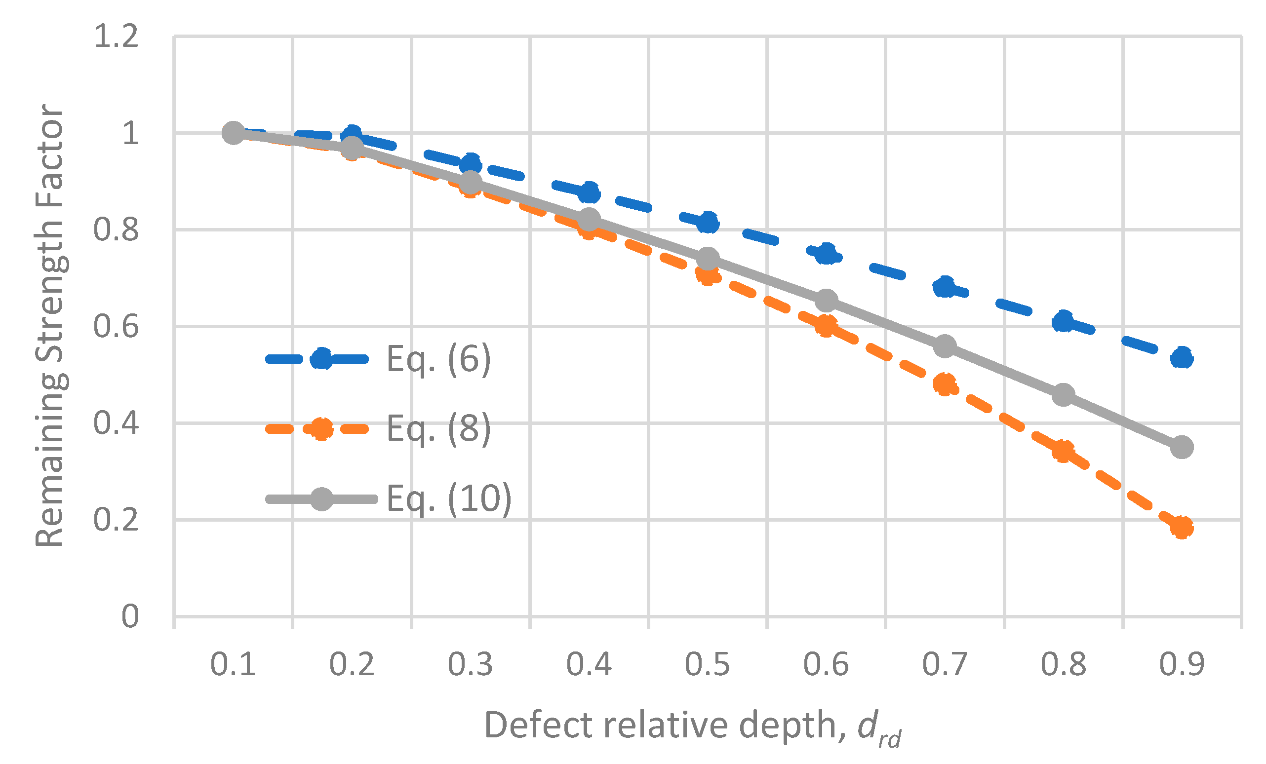
  • The original method from the American Standard ASME B31.G [36], based on the following equations:
    R S F = { 1.1 1 2 3 d r d 1 2 3 · d r d M for   s r d 2 20 1.1 · ( 1 d r d ) for   s r d 2 > 20
    where:
    M = 1 + 0.8 s r d 2
  • The method recommended by DNV RP-F101 [37], using the equations:
    R S F = 1.1 1 d r d 1 d r d M
    in which:
    M = 1 + 0.31 s r d 2 .
  • The modified method from B31.G [36], based on the equations:
    R S F = 1.1 1 0.85 d r d 1 0.85 d r d M
    where:
    M = { ( 1 + 0.6275 s r d 2 0.003375 s r d 4 ) 1 / 2 for   s r d 2 50 0.032 s r d + 3.3 for   s r d 2 > 50 .
In all Equations (6)–(11), M is the bulging stress magnification (Folias) factor.
The maximum (safe) operating pressure of the damaged pipeline, pd, required for the design of the composite wrap, can be evaluated using the RSF, with the equation:
pd = RSF pao
The reinforcement effect of a composite wrap applied to repair a damaged pipeline is mostly a function of the mechanical properties of the composite material and of the wrap dimensions (thickness and length). Therefore, in order to optimize such effect, a proper selection of the composite wrap and an adequate design (definition of its optimal dimensions) is needed. For that reason, the methods most used at the moment for the composite wrap design have been investigated.
The design procedure for a composite repair system comprises the following stages [22,23]:
(1)
Evaluation of the mechanical strength of the damaged pipe (normally by calculating its RSF) and assessment of the opportunity of the repair, based on the criteria detailed in [1,34,35];
(2)
Selection of the type of composite material wrap used for repair;
(3)
Design of the composite wrap geometry, i.e., definition of its characteristic dimensions (thickness, tcw, and length, lcw);
(4)
Verification of the design solution obtained at stage 3, based on the scheme developed in [22,23];
(5)
Final confirmation and adjustment/correction of the design solution (proposed values for tcw and lcw), using eventually a finite elements numerical analysis.
For the definition, at stage 3, of the composite wrap thickness, tcw, the most frequently used methods available in literature have been analyzed and commented by the authors in [21,22,23]. In addition, a new calculation method has been proposed and developed in [22,23]. In the present analysis, we have aimed at identifying the most adequate method, among the following five (in all cases, it is assumed that no additional loads are applied to the repair pipeline):
  • The method defined in [29] (as Design Methodology for Underlying Substrate Does Not Yield) and [38] (as Design Based on Substrate—Allowable Stress): the minimum required value for the composite thickness shall be calculated as the maximum resulting from the following two equations:
    t c w = D e 2 E p E c c 1 σ a p ( p c p d )
    t c w = D e 4 E p E a c 1 σ a p ( p c p d )
  • The method defined in [29] (as Design Methodology for Underlying Substrate Yields) and [38] (as Design Based on Repair Laminate – Allowable Strains), based on the following equation:
    t c w = 1 E c c · ε a c c ( p c · D e 2 σ a p · t m m )
  • The method proposed in [39], by the manufacturer of the type V composite material, based on the following equation (processed by the authors):
    t c w = t n R y p R m c c f d ( 1 R S F ) f f t
  • The method based on the formulation proposed by Alexander in [40] for the assessment of the bursting pressure of a pipeline repaired with a composite wrap, resulting in the equation:
    t c w = t n R m p R m c c 1 f f t [ 2 ( 3 ) n s p + 1 1 1 2 t r p + d r d 1 ]
    where:
    n s p = 0.224 ( R m p R y p ) 0.604
  • Finally, the method developed by the authors [21,22,23]: considering the pipe a multi-layered tube (with the composite wrap as the outer layer and an equivalent steel pipe as the inner layer) and formulating the analytical condition for this tube to withstand the pressure pc, it results:
    t c w = D e 2 [ K E P μ c + 1 K E P μ c 1 1 ]
    in which:
    K E P = E c c E p 1 k e p 2 1 [ 8 t r p k e p 2 t r p ( 3 k e p 2 + 1 ) k e p 2 + 1 K E P 0 ] , K E P 0 = ( k e p 2 1 ) ( 1 μ p ) + 2 ,   K e P = b e p a e p ,
    where aep and bep are respectively the internal and external radius corresponding to an equivalent pipe without any defect, made of the same steel as the damaged pipe, defined as having the same mechanical strength as the pipe area with defect. The values of aep, bep and the wall thickness of this equivalent pipe, tep, are obtained using the following equations:
    a e p = D e 2 t e p ,   b e p = b p ,   t e p = p d 2 σ a p + p d D e .
The analyses described in [21] led to the conclusion that Equation (16) always provided relatively low, optimistic estimations for the composite wrap thickness. Therefore, we consider that the design method based on this equation is not a reliable one and, as a consequence, has not been considered for the additional investigations detailed in the present paper.
The design methods defined in [29,38] are valid only for values of the composite wrap thickness, tcw, not greater than De/6, as specified in [38]. Consequently, in all the analyses results presented in this paper, the tcw values considered have been limited to De/6.
The length of the composite wrap, lcw, can be calculated using the following equation [29,38]:
lcw = sp + 2(stl + sol),
in which sol is the overlap length, corresponding to the distance with which the composite wrap over-distances (on both sides of the pipe, in the axial direction) the defect, and stl is the taper length, corresponding to the projection on the pipe axial direction of the bevel from each wrap extremity. The values of stl and sol can be adopted, if no additional loads are considered, as follows [29,38]:
s o l = max [ 1.77 D e t n ; 38   mm ] , s t l 1.1 t c w .
The finite element simulations aimed, among others, at the identification of the most acceptable composite design method from the ones described above, by comparing the numerical results with the values obtained using Equations (13)–(15) and (17)–(21) respectively.

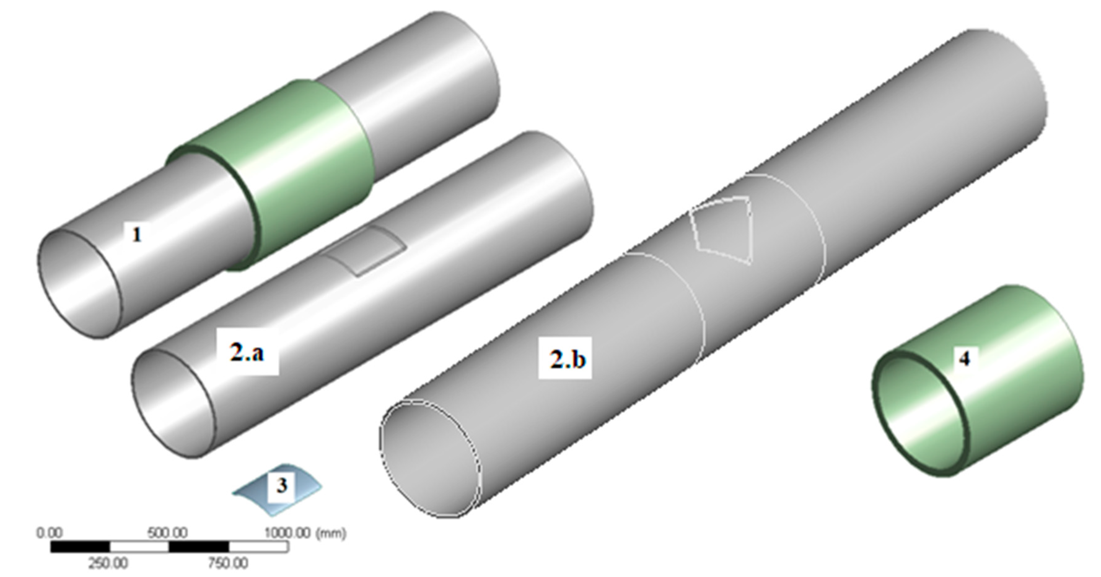
4. Investigated Case Studies

The finite element investigations of the stress-strain state in the repaired pipe area have been performed for two relevant case studies, detailed in [21]. The same pipe material has been selected for both cases, an X42/L290 steel, considered the most adequate for our investigations, as it ranges among the ones frequently used in the older pipelines systems (usually requiring repair works).
We have assumed that the mechanical properties of the selected steel grade equal the specified minimum values from the ISO standard [41], i.e.: Ryp = 290 MPa and Rmp = 415 MPa. The corresponding allowable stress value, calculated with the first Equation (4), assuming fd = 0.72, results: σap = 209 MPa.
The pipe data selected for the case studies are summarized in Table 2, together with the dimensions assumed for the metal loss defect considered on each pipe. The values selected for the pipe outside diameter range among the ones frequently used: De = 219.1; 323.9; 508.0; 711.0 mm.
The design pressure has been evaluated using the following equation, as required by [42]:
p c = 2 · R y p · t n D e f d · f L · f T ,
where fL is the longitudinal joint factor, and fT the temperature derating factor (both assumed equal to 1 for the cases investigated), while fd = 0.72, as previously mentioned in Section 4.
The defect has been assumed to have a rectangular shape, as shown in Figure 2b–d. Such an assumption is based on the fact that, during the repair process, in all cases, a corrosion defect, normally having an irregular shape (an example is included in Figure 2a), is machined and rounded in a manner that generates a rectangular shape with smoothed corners, including the entire corroded area, as described in Figure 2b,c, in order to eliminate the stress concentration effect.
With respect to the investigations from [21], only three values of the defect maximum depth, dmax, have been considered for the additional analyses. The values indicated in Table 2 for the defect actual width, wp (which is not taken into account by any composite design method as its influence is considered minor—see Section 3) are medium values for typical metal loss defects. However, a sensitivity analysis of its influence upon the stress distribution in the repaired steel pipe has been performed using finite elements simulation, for case study no. 1 (De = 323.9 mm) and type III composite material, the results being described at the end of Section 5.
In addition, a sensitivity analysis has been performed in order to assess the influence of the defect orientation (with respect to the steel pipe axis) on the state of stress within the pipe. Normally, the edges of the rectangular metal loss defect, obtained after machining, are oriented parallel/perpendicular with respect to the pipe axis, as shown in Figure 2c. In this paper, a defect with such orientation has been named “straight” defect. However, the authors propose another approach for the defect machining process, resulting in a rectangular shape with its edges inclined with respect to the pipe axis. The dimensions and orientation of the resulting rectangle (named in the followings “inclined” defect) are chosen such as it has the smallest possible dimensions [43]. Its orientation has been measured by the angle α between the edges of the defect and the pipe longitudinal axis, as defined in Figure 2d (which presents the inclined defect with its dimensions).
While for a straight defect (Figure 2c) its axial extent, sp, equals its actual length, lp, and its circumferential extent, cp, equals its actual width, wp, in the case of an inclined defect (Figure 2c), they differ (splp, cpwp). The amplitude of such difference depends on the angle α and we believe it should be taken into account when calculating the composite thickness in the design process, in which the axial/longitudinal extent of the defect is to be considered and not its actual length. The results of the sensitivity analyses on the defect orientation are presented and discussed in Section 6, together with a similar analysis regarding the value of the fillet radius used when machining the defect bottom edges and rounded corners.
The RSF has been calculated for both cases and srd = 3.6, for values of drd ranging between 0.1 and 0.9, using the relevant three methods previously presented. As it can be seen from Equations (6)–(11), the RSF values are depending only on the defect dimensions (depth and length) and therefore they are the same for both pipe dimensions considered in our analyses. Figure 3 shows these values as a function of the relative depth, drd.
As it can be seen from Figure 3, the most conservative evaluation of the RSF value was given by Equation (8), but the values obtained with Equation (10), that we consider to be the most accurate one, are relatively close. In addition, it can be observed that defects with drd = 0.1…0.2 do not require repair (as either RSF >1 and pd = pc or RSF is greater than its allowable value, RSFa, usually considered equal to 0.9 [1,34,35]) and therefore they have not been furtherly analyzed.
The values assessed for the safe operating pressure, based in each case on the lowest RSF value indicated in Figure 3, are presented in Figure 4, as a function of the relative depth, drd.
For the drd values indicated in Table 2, the composite thickness required for the pipeline repair has been calculated, for both cases studied and the composites types included in Table 1, applying successively the four methods described by the Equations (13)–(15), (17) and (19). The results obtained have been also verified according to stage 4 from the design methodology described in [22,23]. Then, they have been compared with the ones of the finite elements simulations mentioned below and the results of this comparison are detailed in [21] and also included in Section 5.

5. Finite Elements Simulations and Results

Finite element simulations have been performed for both cases, considering the data from Table 2, assuming a minimum feasible value for the composite thickness of 10 mm, and using the model described in Figure 5. These simulations, detailed in [21], were aimed at obtaining the optimal composite thickness value, defined as the one for which the maximum value of the stress encountered in the steel pipe wall equals the allowable stress value, i.e., σap = 209 MPa. In such case, we have considered that the pipe mechanical strength has been fully restored to the level corresponding to the undamaged pipe (without any defect).
Finite Elements Analyses (FEA) have been performed using the ANSYS software, taking into account the combined system: steel pipe—polymeric filler (applied only in the defect area)—composite material wrap. Only linear analyses have been performed, as the maximum equivalent stress value in the steel pipe was always below its yield strength (Ryp = 290 MPa).
The pipe, in all our analyses, has been assumed as fixed at both ends. This condition is the closest to the real conditions of the pipe (usually buried). In order to diminish the effect of the fixed ends on the stress distribution in the defect area, the length of the pipe segment has been set to 2240 mm.
The following three approaches have been considered for the finite elements mesh:
  • − non-linear mechanical mesh, with Curvature proximity and Capture curvature ON;
  • − non-linear mechanical mesh, with Curvature proximity and Capture curvature OFF;
  • − mechanical mesh.
The above settings produced, respectively 4,638,571, 2,435,085 and 1,043,163 elements. Sizing and share topology conditions have been used. Although the difference in number of elements is quite important, the results were, for the cases considered, identical (differences only after the decimal point have been observed). Tests have been performed with the smoothing set on low, medium and high. Insignificant differences were reported, though Smoothing on Low has been used.
For all the settings mentioned above, the element quality, aspect ratio and skewness were analyzed and were almost identical. Figure 6 and Table 3 present an example for the element quality.
The above considerations determined the authors to perform all the analyses using the mechanical element type, sizing controls and share topology. The element type used was tetrahedral.
For the elements’ sizes, the authors have used values able to assure a good aspect ratio, as reflected in the quality mesh metric. In order to assess the element size influence on the results, Figure 6d includes a plot proving that, with the used elements sizes and settings (adaptive sizing), the results remain practically constant.
The mechanical properties assumed for the filler have been selected based on the optimal values defined in [32]: Young modulus Ef = 30 GPa; tensile strength Rmf = 60 MPa.
Figure 7 shows, as an example, the FEA results for a pipeline (De = 323.9 mm, tn = 9.5 mm) with a straight local metal loss defect, with the depth dmax = 4.75 mm and the axial extent sp = 220 mm, repaired with a type III fiberglass composite wrap with the thickness tcw = 23 mm.
Figure 8 and Figure 9 indicate a summary of the comparison between the analytical and FEA results, detailed in [21], of our analyses for both cases studied (as defined in Table 2) and for all five types of composite material indicated in Table 1, in terms of the dependence between the minimum composite wrap thickness needed, tcw, and the relative depth of the defect, drd.
The composite thickness values larger than the acceptable limit De/6, defined in Section 4 (i.e., 55 mm for De = 323.9 mm, and 120 mm for De = 711 mm), have not been include in Figure 8 and Figure 9, with only two exceptions. As a consequence, only the results for drd = 0.3 have been shown for type II composite (characterized by relatively low values of the Young modulus). For larger values of the defect relative depth, the required tcw values were found to be well beyond the De/6 limit and therefore it is not advised to repair steel pipes with drd > 0.3 using type II composite.
Analyzing the results from Figure 8 and Figure 9, it can be noticed that the design method based on Equations (13) and (14) gives the best assessment of the composite thickness (i.e., the values for tcw closest to FEA results) for both type I and III composite repair systems, while Equation (17) gives the best evaluation for the type IV composite. For the case of type II composite, Equation (19) provides the closest tcw values to the FEA results, but these results indicate larger composite thickness values than all analytical design methods. The last statement is also valid for type V composite system, but in this case both Equations (13), (14) and (19) provides the closest values of tcw to the FEA results.
If comparing only types I to IV of the composite repair systems investigated, type IV (the only one armed with aramid fibers) appears to be the best solution from the point of view of the thickness required, closely followed by type I and III. As type V composite is armed with carbon fibers and therefore it could generate additional corrosion processes in the steel pipe, it has not been included in this final comparison even if it would require the minimum thickness values.
In addition to the results detailed in [21], a sensitivity analysis regarding the effect of the defect width on the state of stress in the steel pipe wall and its influence upon the composite wrap design process has been performed. Such FEA has been made for case study no. 1 (De = 323.9 mm, steel grade X42), type III composite and a straight defect (for which the actual width equals its circumferential extent, cp) with dmax = 4.75 mm (drd = 0.5). Defects with a smaller/larger width, equal to 10 mm (narrow defect), 100 mm and 220 mm, have been considered, in addition to the width initially assumed in this case (150 mm, as shown in Table 2). Furthermore, two different values have been used for the defect length (axial extent, sp), 111 mm and 277 mm. In all cases, the same thickness value has been assumed for the composite wrap: tcw = 30 mm. This value is approximately equal to the maximum one defined by the analytical methods for De = 323.9 mm, drd = 0.5 and type III composite, value given by Equations (13) and (14) and the closest one to the FEA result (as it can be seen in Figure 7).
Scheme 1 presents comparatively the numerical results obtained, including the maximum value of the von Mises equivalent stress resulting from FEA in each case, σM,max, and the relative difference, RD (in %), between σM,max value and the allowable stress limit, σap = 209 MPa, defined in Section 4. The relative difference RD values, which can also be negative since we can obtain, as FEA results, for a given case, σM,max values greater or smaller than the σap limit, have been calculated as follows:
R D = σ M , max σ a p σ a p 100 [ % ]
The results summarized in Scheme 1 demonstrate that there is a small influence of the defect width on the state of stress in the repaired steel pipe, as the relative difference RD between the maximum and allowable stress values ranges between +/− 1.9% and 13.9%, most values being under 5%. As a consequence, the results obtained using analytical methods (which do not take into account the actual width of the metal loss defect) for the assessment of the composite wrap thickness, tcw, required to repair a damaged steel pipe, are affected only in a small measure by the actual value of the defect width.

6. Sensitivity Analysis of the Defect Orientation and Fillet Radius

The authors considered of interest to investigate additionally the influence of the defect fillet radius used when machining the damaged pipe area (see Figure 2) and of the defect orientation upon the stress distribution in the steel pipe wall.
The same type of finite element analysis as the one presented in Section 5 for the straight defects, i.e., machined to be oriented along the pipe axis (α = 0 degrees, see Figure 2d), has been performed, but only for type II and III composites included in Table 1 (being the ones most frequently used at present for steel pipe repair). For the inclined defects, three values of the inclination angle (defined in Figure 2d) have been considered: α = 45, 60, 75 degrees.
The stress distribution in the defect area has been investigated using FEA for both cases considered in Table 2 (323.9 mm and 711 mm steel pipes) and for the three relative defect values indicated in the same table. However, for type II composite, only the smallest defect depth (drd = 0.3) has been considered, because the required wrap thickness calculated for larger defect depth values did not fulfil the condition tcw < De/6, mentioned in Section 3. A great number of cases have been analyzed, only the most relevant ones being discussed in this section.
The approach used in our sensitivity analysis comprised the following two stages:
  • At first, a composite wrap thickness, tcw, has been calculated analytically (based on the allowable stress limit, as defined in Section 4, σap = 209 MPa) in each case, using the same four methods as for straight defects, described by the Equations (13), (14), (15), (17) and (19), but considering the defect axial extent sp, which is not equal, if α ≠ 0, with its actual length, lp;
  • Then, a finite element analysis has been performed, considering in each case the highest tcw value from the four assessed with the analytical methods used, and the results (in terms of von Mises equivalent stress values) have been compared with the case of the straight defect.
We have decided to consider, in our finite elements sensitivity analysis, the composite wrap thickness given by the analytical method that assesses, for each composite type considered, the greatest tcw values because, as it can be seen in Figure 8 and Figure 9, FEA usually provided higher, more conservative tcw values. Therefore, for type III composite, Equations (13) and (14) have been used, as they give the highest wrap thickness values, while for type II composite, the values calculated with Equations (19)–(21) have been considered.
Figure 6 (in Section 5) presents details of the finite elements mesh in the defect area (Figure 6a), in the filler and composite wrap (Figure 6b), information about the mesh quality (Figure 6c) and the results of the elements size influence assessment, commented in Section 5 (Figure 6d). As mentioned in Section 5, from the geometric modeling stage, share topology has been used to assure a good compatibility between the meshes of the components (pipe, filler and composite).
Figure 10 presents the stress distribution (equivalent von Mises) for one of the considered cases: steel pipe with 323.9 mm exterior diameter and inclined defect at 45 degrees, with a 0.3 relative depth.
In all cases analyzed, as it can be also seen in Figure 10b,c, the maximum values of the equivalent von Mises stress determined by FEA for the composite material and for the filler was found to be below or even well below the allowable stress values for these materials.
In the following, we discuss separately the sensitivity analysis results regarding the influences on the stress distribution in the steel pipe wall of the following parameters:
  • fillet radius at the defect bottom edges and at its corners;
  • defect orientation with respect to the longitudinal axis of the steel pipe;
  • defect relative depth.

6.1. Influence of the Fillet Radius on the Stress Distribution

In order to assess the influence of the fillet radius used when machining the defect bottom edges and its corners (we have considered the same radius value for all edges and corners), for each case analyzed four situations have been considered: the fillet radius is equal with the maximum defect depth value multiplied by 2, 4, 6 or 8. This sensitivity analysis has been performed for both pipe diameter values considered, 323.9 and 711 mm, for type III composite, using Equations (13) and (14) to assess its thickness, and type II composite, using in this case Equations (19)–(21) to assess its thickness.
For these cases, the equivalent von Mises stresses have been evaluated. Figure 11 presents, as an example, the results obtained, for both steel pipes investigated, for type III composite, and for a relative defect depth drd = 0.3. Similar results (not included in the present paper) have been obtained for all the other drd values considered and also for type II composite. The tendencies in all these cases have been found to be similar with the ones that can be observed in Figure 11.
The results of our analysis evidently indicate that, when the fillet radius increases, the equivalent stress decreases. FEA have been also performed for values of the radius multipliers greater than 8, but it has been noticed that the stress tendency to decrease is likely to flatten.
The results have been analyzed in order to assess if, for given values of the defect relative depth or orientation angle, the observed decrease of the maximum equivalent stress is more significant. It can be clearly noticed that, for straight defects (α = 0 degrees) and for inclined defects with α = 75 degrees, the tendency of the equivalent stress to decrease, when the defect depth increases, is less significant. Such tendency was found to be similar for both pipes (De = 323.9 and De = 711 mm) and for both composites (type II and III).

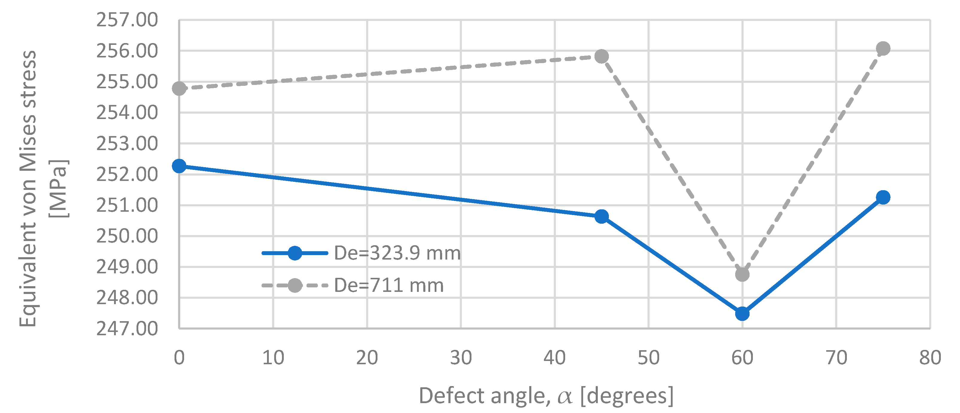
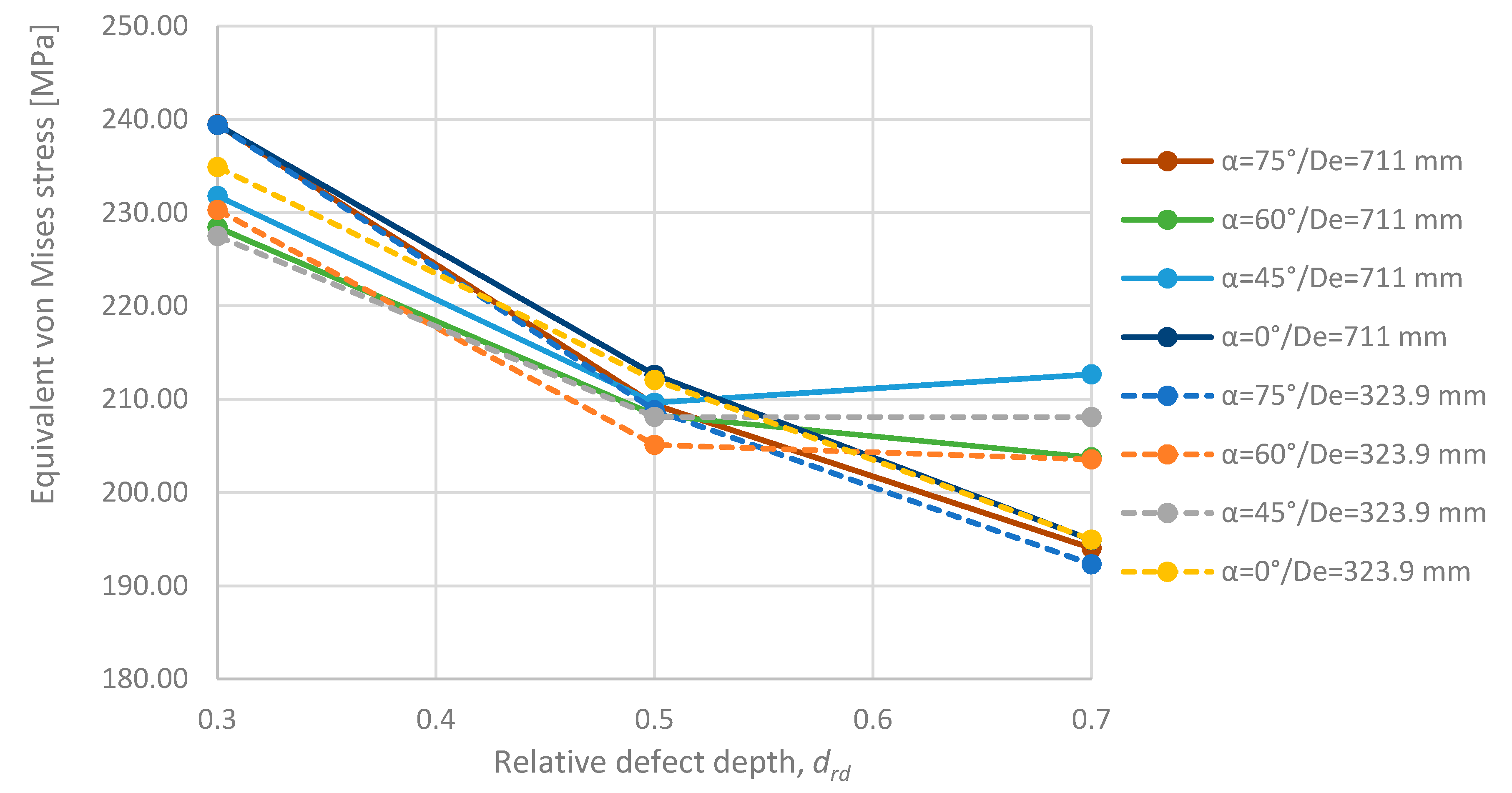
6.2. Influence of the Defect Orientation on the Stress Distribution

In order to assess the influence of the defect orientation, the dependence of the maximum von Mises equivalent stress versus the defect angle has been shown in Figure 12 and Figure 13. As already mentioned, the wrap thickness considered in the FEA has been calculated using Equations (13) and (14) for type III composite (Figure 12) and with Equations (19)–(21) for type II composite (Figure 13). The greatest value for the fillet radius multiplier (8) has been considered to assess the stress distributions as this value leads to the smallest value for the maximum equivalent stress.
The analysis of Figure 12 and Figure 13 allowed us to make the following statements:
  • The general equivalent stress variation tendencies for a given relative defect depth are similar for both steel pipes considered and for both composite types;
  • For the relative defect depths of 0.3 and 0.5, the equivalent stress tends to decrease with the defect orientation, up to the inclination angle of 60 degrees (which corresponds to the largest axial extent value), followed by an increase for the 75 degrees angle; this is valid for both composite types;
  • For the relative defect depth of 0.7, the equivalent stress increases with the defect inclination angle up to 45 degrees, then it decreases for the following angle values: 60 and 75 degrees.

6.3. Influence of the Defect Depth on the Stress Distribution

The influence of the defect depth on the equivalent von Mises stress maxima (in the defect area) are shown in Figure 14, for type III composite. The FEA results have been obtained for all considered defect orientations using the composite thickness defined by Equations (13) and (14). The greatest value for the fillet radius multiplier (8) has been used to determine the stress distributions.
This influence has not been analyzed for type II composite as the analytically calculated composite thickness values satisfy the condition tcw < De/6 only for the smallest defect depth (the only one considered in our investigations).
The analysis of Figure 14 allows us to state that there is a clear tendency for the defects with extreme values in orientation (α = 0, respectively α = 75 degrees) to present a decreasing tendency while defect depth is increasing. For the other two inclinations (45 and 60 degrees) stresses decrease when defect depth increases up to drd = 0.5 for both pipes considered. Beyond these values, the stress values remain constant of slightly increase.
Finally, we have evaluated the concordance of the results obtained using the analytical methods to assess the composite thickness and the finite element analysis results. Our purpose has been to appreciate the accuracy of the analytical results, for all cases considered (steel pipe diameter, defect depth and orientation etc.), by analyzing the stress distribution in the defect area evaluated using the finite element method for the composite thickness value assessed using the analytical method which gives the highest tcw values, that is (as previously mentioned) the one based on Equations (13) and (14) for type III composite and on Equations (19)–(21) for type II composite.
To that purpose, the relative difference, RD (in %), between the maximum equivalent von Mises stress value assessed by FEA, σM,max, and the allowable limit (σap = 209 MPa), as defined by Equation (25), has been calculated. The greatest value for the fillet radius multiplier (8) has been used for the stress distributions. The results are summarized in Figure 15 and Figure 16 for type III and II composites respectively.
In some cases, negative values have resulted for RD, as the values obtained for σM,max as FEA results were smaller than the allowable limit. This was mainly the case of type III composite and the defect with drd = 0.7 (see Figure 15). Such results indicate a good prediction of the composite wrap thickness given by the analytical method applied in these cases, based on Equations (13) and (14).
The analysis of our results reveals that a good concordance between the analytical method and the FEA results was obtained for type II composite, using Equations (13) and (14) to calculate the composite thickness needed, and for the medium depth defects (for both pipes), as shown in Figure 15, while the defect orientation had a smaller effect. A not so good concordance has been obtained for type II composite and the use of Equations (19)–(21) to assess the thickness (see Figure 16). Since in this case only the defects with the smallest depth have been considered, the influence of the defect orientation has been more noticeable, a better concordance being obtained for the defect oriented at 60 degrees.

7. Conclusions

The investigations described in this paper and in [21] have led to the following main conclusions regarding the repair method using composite materials wraps for the reinforcement of the steel pipe areas with local metal loss defects:
  • The repair method investigated is advantageous, allowing for operative maintenance works without removing the pipeline from service. However, at present, there is no design method widely accepted for the definition of the characteristic thickness of the composite wrap, tcw.
  • The composite repair systems using materials with greater values of the tensile strength and especially of the Young modulus (having values closer to the ones of the steel) are more effective in restoring the mechanical strength of a damaged (corroded) pipeline.
  • The results of the analyses detailed in [21] showed that the most adequate method for the composite wrap thickness design (giving the closest results to FEA simulations) are the one proposed by the ASME and ISO norms [29,38], using Equations (13) and (14), followed by the one developed by the authors in [22,23], based on Equation (19).
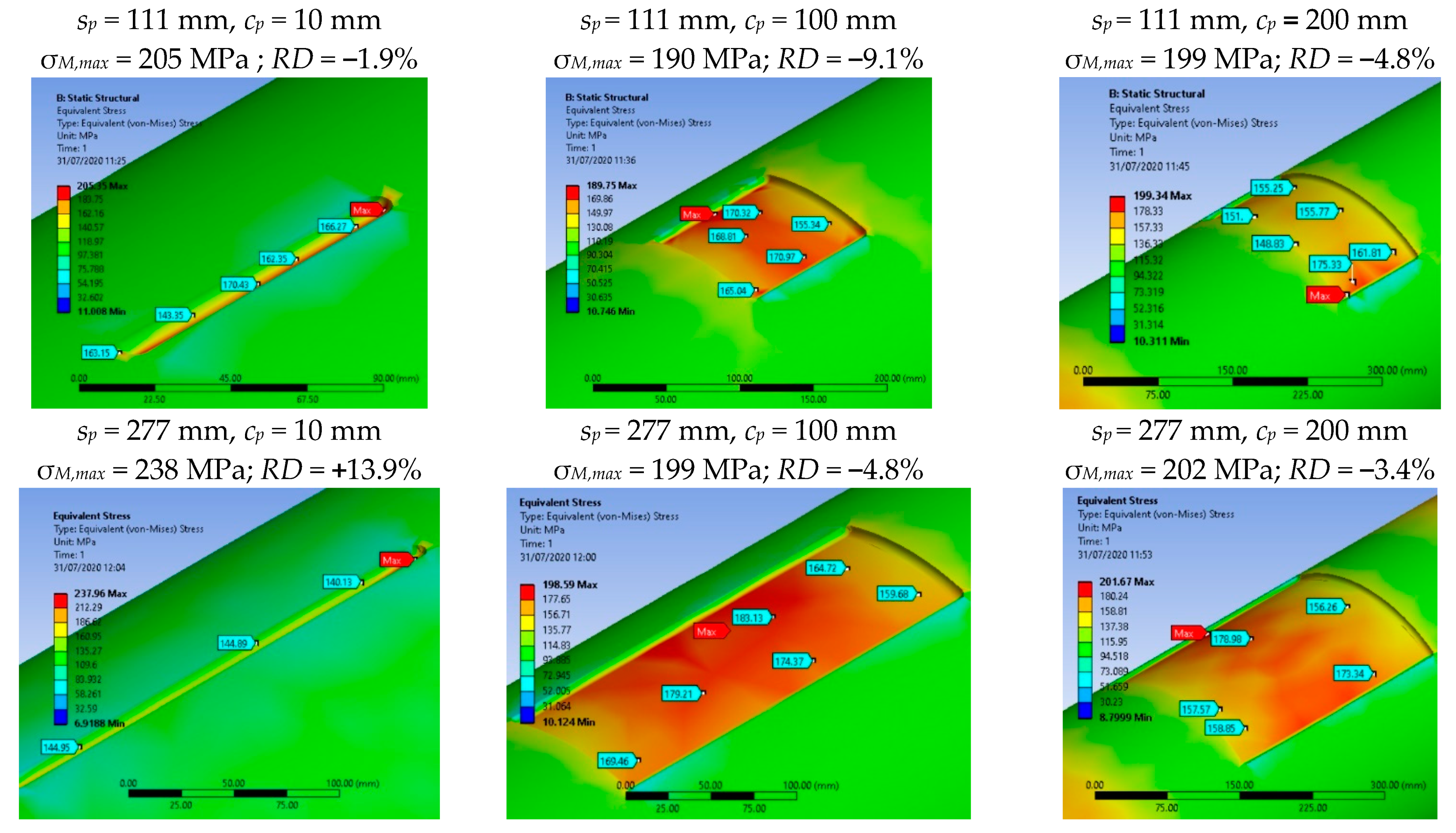
  • As our FEA investigations have proven that the influence of the actual width of the metal loss defect on the state of stress in a steel pipe repaired using composite materials is relatively small, the composite wrap thickness needed for repair can be safely assessed using the analytical methods mentioned in this paper, even if they do not consider the defect width value.
  • The finite elements analysis of the influence of the defect orientation and fillet radius (used to machine the damaged pipe area) upon the stress distribution have demonstrated the following:
    It is useful to decide on machining the defect area as an inclined rectangle, as it will reduce the workload without not affecting the pipe safety;
    The angle of the defect orientation (excluding the straight defect case) influences the maxima for the equivalent von Mises stress, but only within a range of around 10%;
    The fillet radius used to machine the bottom of the defect and its corners has a significant influence on the stress distribution for all considered defect orientations;
    In the case of inclined defects, the maxima for the equivalent von mises stress migrates towards the rounded corners (as can be seen in Figure 10);
    The FEA results reveals good concordance with the analytical results when using Equations (13) and (14) to assess the wrap thickness for type III composite.
In the future, the authors intend to analyze, both numerically and experimentally, additional cases, considering various composite repair systems, defect geometries and orientations, steel grades and pipe dimensions, in order to define the optimal composite design method in each case. Furthermore, the effect of additional axial loads and temperature variations will be also investigated. We plan to study as well the use of composite wraps to repair steel pipes with crack-like defects and to analyze the crack propagation phenomenon using fracture modeling.

Author Contributions

Conceptualization, A.D. (Andrei Dumitrescu) and M.M.; methodology, A.D. (Andrei Dumitrescu); software, A.D. (Alin Dinita) and I.L.; validation, A.D. (Alin Dinita) and I.L.; formal analysis, A.D. (Alin Dinita) and I.L.; resources, M.M.; data curation, A.D. (Andrei Dumitrescu); writing—original draft preparation, A.D. (Andrei Dumitrescu); writing—review and editing, A.D. (Alin Dinita); visualization, I.L.; supervision, M.M.; project administration, A.D. (Andrei Dumitrescu). All authors have read and agreed to the published version of the manuscript.

Funding

This research has received funding from the European Union Seventh Framework Program FP7-PEOPLE-2012-IRSES, grant agreement n° 318874 “INNOPIPES—Innovative Nondestructive Testing and Advanced Composite Repair of Pipelines with Volumetric Surface Defects”.

Informed Consent Statement

Not applicable.

Data Availability Statement

The data presented in this study are available on request from the corresponding author.

Conflicts of Interest

The authors declare no conflict of interest. The funders had no role in the design of the study; in the collection, analyses, or interpretation of data; in the writing of the manuscript, or in the decision to publish the results.

Nomenclature

Accelongation at break of the composite material in the circumferential direction
apinternal radius of the steel pipe
bpexternal radius of the steel pipe
cpmetal loss defect circumferential extent
Desteel pipe outside diameter
dmaxmaximum depth of the metal loss pipe defect
drd = dmax/tnrelative depth of the metal loss defect
EacYoung modulus of the composite material in the axial direction
EccYoung modulus of the composite material in the circumferential direction
EpYoung modulus of the steel pipe
fservice factor used for composite design
fttemperature derating factor, used for composite design
fdpipe design factor
lcwcomposite wrap length
pao = MAWP/MAOPmaximum allowable working / operating pressure of the steel pipe
pcpipe design pressure
pd = RSF paomaximum (safe) operating pressure for a steel pipe with defects
Rmptensile strength of the steel pipe
Rmccshort-term tensile strength of the composite material in the circumferential direction
Rmclclong-term tensile strength of the composite material in the circumferential direction (defined as being greater or equal to 1000 h)
RSFRemaining Strength Factor (of a damaged/corroded steel pipe)
Rypyield strength of the steel pipe
spmetal loss defect longitudinal / axial extent
srdrelative length of the metal loss defect
tcwcomposite material wrap thickness
tnnominal wall thickness of the steel pipe
trp = tn/Desteel pipe relative thickness
εaccallowable (long-term) strain of the composite material in the circumferential direction
σaccallowable (long-term) stress of the composite material in the circumferential direction
σapsteel pipe allowable stress
μpPoisson ratio of the steel pipe
μcPoisson ratio of the composite material in the circumferential direction

References

  1. Dumitrescu, A.; Zecheru, G.; Diniță, A. Characterisation of Volumetric Surface Defects. In Non-Destructive Testing and Repair of Pipelines; Barkanov, E.N., Dumitrescu, A., Parinov, I.A., Eds.; Springer International Publishing AG: Cham, Switzerland, 2018; pp. 117–135. [Google Scholar]
  2. Zecheru, G.; Bârsan, M.F.; Drăghici, G.; Dumitrescu, A. Technological solutions for preventing hydrogen induced cracking when repairing by welding hydrocarbons transmission pipelines—Part I. Sudura 2015, XXV-4, 20–45. [Google Scholar]
  3. Zecheru, G.; Bârsan, M.F.; Drăghici, G.; Dumitrescu, A. Technological solutions for preventing hydrogen induced cracking when repairing by welding hydrocarbons transmission pipelines—Part II. Sudura 2016, XXVI-1, 14–39. [Google Scholar]
  4. Zhao, W.; Zhang, T.; Wang, Y.; Qiao, J.; Wang, Z. Corrosion Failure Mechanism of Associated Gas Transmission Pipeline. Materials 2018, 11, 1935. [Google Scholar] [CrossRef] [Green Version]
  5. Mansoori, H.; Mirzaee, R.; Esmaeilzadeh, F.; Vojood, A.; Dowrani, A.S. Pitting corrosion failure analysis of a wet gas pipeline. Eng. Fail. Anal. 2017, 82, 16–25. [Google Scholar] [CrossRef]
  6. Zhang, H.; Lan, H.Q. A review of internal corrosion mechanism and experimental study for pipelines based on multiphase flow. Corros. Rev. 2017, 35, 425–444. [Google Scholar] [CrossRef]
  7. Ifezue, D. Root cause failure analysis of corrosion in wet gas piping. J. Fail. Anal. Prev. 2017, 17, 971–978. [Google Scholar] [CrossRef]
  8. Kovalenko, S.Y.; Rybakov, A.O.; Klymenko, A.V.; Shytova, L.H. Corrosion of the internal wall of a field gas pipeline. Mater. Sci. 2012, 48, 225–230. [Google Scholar] [CrossRef]
  9. Mirshamsi, M.; Rafeeyan, M. Speed control of inspection pig in gas pipelines using sliding mode control. J. Proc. Control 2019, 77, 134–140. [Google Scholar] [CrossRef]
  10. Li, X.; Zhang, S.; Liu, S.; Jiao, Q.; Dai, L. An experimental evaluation of the probe dynamics as a probe pig inspects internal convex defects in oil and gas pipelines. Measurement 2015, 63, 49–60. [Google Scholar] [CrossRef]
  11. Xie, M.; Tian, Z. A review on pipeline integrity management utilizing in-line inspection data. Eng. Fail. Anal. 2018, 92, 222–239. [Google Scholar] [CrossRef]
  12. Li, X.; Zhang, S.; Liu, S.; Zhu, X.; Zhang, K. Experimental study on the probe dynamic behaviour of feeler pigs in detecting internal corrosion in oil and gas pipelines. J. Nat. Gas Sci. Eng. 2015, 26, 229–239. [Google Scholar] [CrossRef]
  13. Bhadran, V.; Shukla, A.; Karki, H. Non-contact flaw detection and condition monitoring of subsurface metallic pipelines using magnetometric method. Mat. Today Proc. 2020, 28, 860–864. [Google Scholar] [CrossRef]
  14. Barkanov, E.N.; Dumitrescu, A.; Parinov, I.A. (Eds.) Non-Destructive Testing and Repair of Pipelines; Springer International Publishing AG: Cham, Switzerland, 2018; pp. 3–106. [Google Scholar]
  15. Wanga, X.; Tse, P.W.; Mechefske, C.K.; Hua, M. Experimental investigation of reflection in guided wave—Base inspection for the characterization of pipeline defects. NDT&E Int. 2010, 43, 365–374. [Google Scholar]
  16. Tse, P.W.; Wang, X. Characterization of pipeline defect in guided-waves based inspection through matching pursuit with the optimized dictionary. NDT&E Int. 2013, 54, 171–182. [Google Scholar]
  17. Clough, M.; Fleming, M.; Dixona, S. Circumferential guided wave EMAT system for pipeline screening using shear horizontal ultrasound. NDT&E Int. 2017, 86, 20–27. [Google Scholar]
  18. Lowea, P.S.; Sandersonb, R.; Pedrama, S.K.; Boulgourisb, N.V.; Mudgeb, P. Inspection of pipelines using the first longitudinal guided wave mode. Phys. Procedia 2015, 70, 338–342. [Google Scholar] [CrossRef] [Green Version]
  19. El Mountassir, M.; Mourot, G.; Yaacoubi, S.; Maquin, D. Damage Detection and Localization in Pipeline Using Sparse Estimation of Ultrasonic Guided Waves Signals. IFAC PapersOnLine 2018, 51–24, 941–948. [Google Scholar] [CrossRef]
  20. Kudina, E.; Bukharov, S.; Sergienko, V.; Dumitrescu, A. Comparative Analysis of Existing Technologies for Composite Repair Systems. In Non-Destructive Testing and Repair of Pipelines; Barkanov, E.N., Dumitrescu, A., Parinov, I.A., Eds.; Springer International Publishing AG: Cham, Switzerland, 2018; pp. 241–267. [Google Scholar]
  21. Dumitrescu, A.; Diniță, A. Efficiency Assessment of the Composite Material Repair Systems Intended for Corrosion Damaged Pipelines. In Proceedings of the 38th International Conference on Ocean, Offshore & Arctic Engineering (OMAE 2019), Glasgow, Scotland, UK, 9–14 June 2019. Paper No. 96279. [Google Scholar]
  22. Zecheru, G.; Drăghici, G.; Dumitrescu, A.; Yukhymets, P. Design of Composite Material Reinforcing Sleeves Used to Repair Transmission Pipelines. PGUP Bull. Tech. Ser. 2014, LXVI, 105–117. [Google Scholar]
  23. Zecheru, G.; Dumitrescu, A.; Diniță, A.; Yukhymets, P. Design of Composite Repair Systems. In Non-destructive Testing and Repair of Pipelines; Barkanov, E.N., Dumitrescu, A., Parinov, I.A., Eds.; Springer International Publishing AG: Cham, Switzerland, 2018; pp. 269–285. [Google Scholar]
  24. Valadi, Z.; Bayesteh, H.; Mohammadi, S. XFEM fracture analysis of cracked pipeline with and without FRP composite repairs. Mech. Adv. Mat. Struct. 2020, 27, 1888–1899. [Google Scholar] [CrossRef]
  25. Abd-Elhady, A.; Sallam, H.E.; Alarifi, I.; Malik, R.; El-Bagory, T. Investigations of fatigue crack propagation in steel pipeline repaired by glass fiber reinforced polymer. Compos. Struct. 2020, 242, 123–130. [Google Scholar] [CrossRef]
  26. Rabczuk, T.; Gracie, R.; Song, J.-H.; Belytscho, T. Immersed particle method for fluid-structure interaction. Int. J. Numer. Methods Eng. 2010, 81, 48–71. [Google Scholar] [CrossRef]
  27. Chau-Dinh, T.; Zi, G.; Lee, P.-S.; Rabczuk, T.; Song, J.-H. Phantom-node method for shell models with arbitrary cracks. Comput. Struct. 2012, 92–93, 242–256. [Google Scholar] [CrossRef]
  28. Zecheru, G.; Dumitrescu, A.; Yukhymets, P.; Dmytriienko, R. Development of an Experimental Programme for Industrial Approbation. In Non-Destructive Testing and Repair of Pipelines; Barkanov, E.N., Dumitrescu, A., Parinov, I.A., Eds.; Springer International Publishing AG: Cham, Switzerland, 2018; pp. 401–416. [Google Scholar]
  29. ASME. Part 4—Nonmetallic and Bonded Repairs. In PCC-2-2015 Repair of Pressure Equipment and Piping; The American Society of Mechanical Engineers: New York, NY, USA, 2015; pp. 139–196. [Google Scholar]
  30. Zecheru, G.; Dumitrescu, A.; Drăghici, G.; Yukhymets, P. Reinforcement Effects Obtained by Applying Composite Material Sleeves to Repair Transmission Pipelines. Mater. Plast. 2016, 53, 252–258. [Google Scholar]
  31. Dmytriienko, R.; Prokopchuk, S.; Paliienko, O. Inner Pressure Testing of Full-Scale Pipe Samples. In Non-Destructive Testing and Repair of Pipelines; Barkanov, E.N., Dumitrescu, A., Parinov, I.A., Eds.; Springer International Publishing AG: Cham, Switzerland, 2018; pp. 417–429. [Google Scholar]
  32. Diniță, A.; Lambrescu, I.; Chebakov, M.; Dumitru, G. Finite Element Stress Analysis of Pipelines with Advanced Composite Repair. In Non-Destructive Testing and Repair of Pipelines; Barkanov, E.N., Dumitrescu, A., Parinov, I.A., Eds.; Springer International Publishing AG: Cham, Switzerland, 2018; pp. 289–309. [Google Scholar]
  33. Lyapin, A.; Chebakov, M.; Dumitrescu, A.; Zecheru, G. Finite-Element Modeling of a Damaged Pipeline Repaired Using the Wrap of a Composite Material. Mech. Compos. Mater. 2015, 51, 333–340. [Google Scholar] [CrossRef]
  34. Zecheru, G.; Yukhymets, P.; Drăghici, G.; Dumitrescu, A. Methods for Determining the Remaining Strength Factor of Pipelines with Volumetric Surface Defects. Rev. Chim. 2015, 66, 710–717. [Google Scholar]
  35. Zecheru, G.; Dumitrescu, A.; Yukhymets, P.; Gopkalo, A.; Mihovski, M. Assessment of the Remaining Strength Factor and Residual Life of Damaged Pipelines. In Non-Destructive Testing and Repair of Pipelines; Barkanov, E.N., Dumitrescu, A., Parinov, I.A., Eds.; Springer International Publishing AG: Cham, Switzerland, 2018; pp. 137–152. [Google Scholar]
  36. ASME. B31G-2009 Manual for Determining the Remaining Strength of Corroded Pipelines; The American Society of Mechanical Engineers: New York, NY, USA, 2009. [Google Scholar]
  37. DNV. RP-F101 Corroded Pipelines. Recommended Practice; Det Norske Veritas A.S.: Hovik, Norway, 2015. [Google Scholar]
  38. ISO. TS 24817:2006 Petroleum, Petrochemical and Natural Gas Industries—Composite Repairs for Pipework—Qualification and Design, Installation, Testing and Inspection. Technical Specification; International Organization for Standardization: Geneva, Switzerland, 2006. [Google Scholar]
  39. Williamson, T.D. RES-Q Wrap Design & Installation of RES-QTM Composite Wrap on Pipelines; T.D. Williamson S.A.: Tulsa, OK, USA, 2012. [Google Scholar]
  40. Alexander, C. Pipeline integrity. Remediation and Repair. In Southern Gas Association Conference, Linking People, Ideas, Information; Southern Gas Association: Houston, TX, USA, 2007. [Google Scholar]
  41. ISO. ISO 3183 Petroleum and Natural Gas Industries—Steel Pipe for Pipeline Transportation Systems; International Organization for Standardization: Geneva, Switzerland, 2007. [Google Scholar]
  42. ASME. B31.8:2009 Gas Transmission and Distribution Piping Systems; The American Society of Mechanical Engineers: New York, NY, USA, 2009. [Google Scholar]
  43. Lambrescu, I. About the Influence of the Machined Defect Shape and Position on the Stress Distribution for Pipelines with Volumetric Defects, The Annals of “Dunărea de Jos” Univ. of Galati, Fascicle IX. Metall. Mater. Sci. 2019, 1, 5–12. [Google Scholar]
Figure 1. Structure of a wet lay-up composite repair system, applied on a steel pipeline [28].
Energies 14 00615 g001
Figure 2. Typical corrosion defect in a steel pipe: (a). an example (before machining); (bd). assumed defect geometry (after machining): (b). transversal section; (c). straight defect (front view); (d). inclined defect (front view); dmax—maximum depth, α—inclination angle with respect to the pipe longitudinal axis; wp—actual width, lp—actual length, sp—axial/longitudinal extent, cp—circumferential extent.
Energies 14 00615 g002
Figure 3. RSF versus relative depth of the defect, drd.
Energies 14 00615 g003
Figure 4. Safe operating pressure, pd, versus relative depth of the defect, drd; steel grade: X42.
Energies 14 00615 g004
Figure 5. FEA general model: 1—steel pipe repaired with a composite system; 2.a—pipe (2 m long) with a straight local metal loss defect (α = 0 deg); 2.b—pipe (3 m long) with an inclined metal loss defect (α = 45 deg); 3—filler (to ensure the load transfer); 4—composite material wrap.
Energies 14 00615 g005
Figure 6. Mesh in the defect area and element metrics: (a). mesh on pipe; (b). mesh on wrap and filler; (c). element quality metric (see also Table 3 below); (d). influence of elements dimensions.
Energies 14 00615 g006
Figure 7. FEA analysis for an X42 steel pipe with a straight local metal loss defect, repaired using type III composite material wrap: De = 323,9 mm; tn = 9,5 mm; dmax = 4.75 mm; sp = 220 mm; Cp = 150 mm; tcw = 23 mm; lcw = 440 mm.
Energies 14 00615 g007
Figure 8. Summary of the results for case study no. 1 (from [21]).
Energies 14 00615 g008
Figure 9. Summary of the results for case study no. 2 (from [21]).
Energies 14 00615 g009
Scheme 1. Sensitivity analysis on the defect width. FEA results.
Energies 14 00615 sch001
Figure 10. Equivalent Von Mises stress distribution: (a). steel pipe (defect area); steel pipe (defect corner – detail); (b). (c). filler; (d). composite wrap. (De = 323.9 mm, drd = 0.3, α = 45 degrees).
Energies 14 00615 g010
Figure 11. Von Mises equivalent stress evolution for several fillet radius multiplier values and defect orientations, for 323.9 mm and 711 mm steel pipes, type III composite, drd = 0.3.
Energies 14 00615 g011
Figure 12. Equivalent von Mises stress maxima for 711 mm and 323.9 mm steel pipes, type III composite and different relative defect depths.
Energies 14 00615 g012
Figure 13. Equivalent von Mises stress maxima for 323.9 mm and 711 mm pipes, type II composite and the relative defect depth drd = 0.3.
Energies 14 00615 g013
Figure 14. Equivalent Von Mises stress maxima for both steel pipes and type III composite.
Energies 14 00615 g014
Figure 15. Relative difference, RD, between the maximum equivalent von Mises stress value and the allowable stress limit, for both pipes and type III composite.
Energies 14 00615 g015
Figure 16. Relative difference, RD, between the maximum equivalent von Mises stress value and the allowable stress limit, for both pipes, type II composite and drd = 0.3.
Energies 14 00615 g016
Table 1. Main mechanical properties of the composite materials intended for pipeline repair.
Type of CompositeIIIIIIIVV
Arming materialglass fibersglass fibersglass fibersaramid fiberscarbon fibers
Tensile modulus Ecc, GPa34.0…38.07.9…8.733.8…34.548.0…49.367.5…69.8
Tensile modulus Eac, GPa7.8…8.7 (a)5 (b)6.1…11.1 (a)18.8…19.626.5…27.4
Poisson’s ratio μc0.30…0.32 (a)0.15…0.230.22…0.250.18…0.190.30…0.33
Shear modulus Gc, GPa3.1…6.5 (a)-3.1…5.94.2…5.56.5…6.8 (a)
Tensile strength Rmcc, MPa580…62072…190630…650188…205822…1020
Elongation at break Acc, %1.0…1.12.8…3.71.0…1.21.3…1.40.25 (c)
(a) only indicative values, defined by analogy with values of the same properties for similar composite materials (the degree of anisotropy is not accurately known); (b) assumed value (not provided by the type II composite manufacturers); (c) value representing the allowable circumferential and axial strain for the composite material.
Table 2. Case studies: pipeline and defect data.
Case Study No.12
Pipeline nominal outside diameter, Demm323.9711
inch12.7528
Nominal wall thickness, tn (a)mm9.520.6
Pipeline design pressure, pc (b)MPa12.212.1
Pipeline MAOP/MAWP, pao (c)MPa12.612.5
Defect relative depth, drd-0.3; 0.5; 0.7
Defect maximum depth, dmaxmm2.85; 4.75; 6.656.18; 10.3; 14.42
Defect actual length, lpmm220440
Defect actual width, wpmm150330
Defect angle, α (d)degrees0; 45; 60; 75
(a) defined by considering the same pipe relative thickness for both pipelines (trp = 0.029); (b) calculated according to the ASME standard [42], as detailed below—see Equation (24); (c) calculated with the second Equation (4); (d) defined as shown in Figure 2 (α = 0 degrees corresponds to a “straight” defect, as defined below).
Table 3. Element quality metric.
Case12345
Average wrap element size [mm]4.158.3121520
Average filler element size [mm]1.4252.855710
Equivalent VonMises stress [MPa]291.3291.33291.24291.29291.26
Publisher’s Note: MDPI stays neutral with regard to jurisdictional claims in published maps and institutional affiliations.

