Article

Fixed Transmission Charges Based on the Degree of Network Utilization

1
Department of Power System and Control, Faculty of Electrical Engineering, Silesian University of Technology, 44-100 Gliwice, Poland
2
Department of Computer Science, Faculty of Electrical Engineering, Automatic Control and Informatics, Opole University of Technology, 45-758 Opole, Poland
*
Author to whom correspondence should be addressed.
These authors contributed equally to this work.
Energies 2021, 14(3), 614; https://doi.org/10.3390/en14030614
Submission received: 3 December 2020 / Revised: 18 January 2021 / Accepted: 22 January 2021 / Published: 26 January 2021

Abstract

:
The core objective of transmission tariffs is the recovery of costs related to the transport of electricity. A usual component of a tariff is a fixed charge that covers the costs of the network infrastructure. As many customers use the power grid, the rate of this charge should reflect, as closely as possible, the actual costs of supplying energy to the individual consumers. These costs result from which network elements have been used in delivering the electricity, and to what extent these elements have been used. Therefore, the fixed transmission rates should depend on the degree of network utilization. This article investigates definitions of the degree of network utilization based on the active power flow. To calculate the degree of network utilization, the flow of electricity on a branch must be decomposed into the streams flowing to individual customers. For this decomposition, two methods are examined: a power flow tracing method, based on the proportional sharing principle, and an incremental power flow method, based on the superposition principle. The analyzed methodology is applied to a small test system for conceptual discussions, as well as to the transmission network of the Polish power system, as an example of practical application. The results of this study were then compared with the commonly used “postage stamp” method. Finally, several practical aspects related to the potential implementation of the presented methodology are discussed.

1. Introduction

1.1. Key Requirements for Transmission Tariffs

The transmission service offered by transmission or distribution system operators consists in transporting electricity from producers to consumers. Transmission is carried out using an electrical grid with different voltage levels. According to the rules currently applied in Poland, and most European countries, a transmission fee is charged to the consumers of electricity [1].
Transmission services differ across consumers due to the fact that individual consumers use energy at different powers, buy different amounts of energy at different times of the day and, above all, utilize different components of the electrical grid, even when they are supplied from the same voltage level. Therefore, the methodology of determining the transmission charges should consider the above differences to the greatest possible extent. A properly constructed transmission tariff should fulfill the following main requirements [2,3]:
  • costs reflectivity–charges paid by individual network users should correspond to the actual costs of the services provided to them; this reflectivity will ensure equal and non-discriminatory access to the network for all entities,
  • price signals–rates of transmission charges should provide information on favorable locations for new generators and large electricity consumers, as well as the required new transmission lines,
  • costs recovery–transmission charges must ensure a level of financial revenue for the network operator that will be sufficient to recover capital and operating costs,
  • simplicity–setting the rates of transmission charges and settling commercial transactions should be transparent and as simple as possible.
Some of the above-mentioned requirements may be difficult to meet at the same time; therefore, when designing transmission tariffs, certain priorities should be established, and the chosen methods of the tariff’s creation should maximize the features that are the most important. First, the tariff creation method should ensure that the rates of transmission charges for individual customers reflect the costs they cause. Additionally, the transmission tariffs should indicate which areas are favorable for the location of new generators, such as areas with a shortage of generated power (i.e., with high costs of transmission service) or areas for connecting potential new customers (i.e., areas with low rates). The tariff should also inform operators what actions may lead to the reduction of transmission costs, and provide an incentive to undertake these actions. The above requirements can be included in one general postulate: the transmission charge should inform, motivate, and cover the costs of electricity transmission.

1.2. Transmission Fixed Costs Allocation Methods

The literature describes several methods of determining transmission charges that meet the above requirements to a greater or lesser extent [4,5,6,7,8,9,10,11,12,13]. The so-called allocation methods that ensure full coverage of transmission costs are the widest group. This article focuses on the fixed costs allocation methods that cover the costs of the network infrastructure. Table 1 contains an assessment of the fulfillment of requirements for the transmission charge for the most common methods.
Generally, the allocation method determines the share in covering the costs of the transmission network for each user. In these methods, the transmission charge is calculated according to a formula:
T C i = T F C s i i s i ,
where TCi is the transmission charge for an i-th network user, TFC is the total fixed costs (the costs of the network infrastructure), and si is a share of the i-th user in covering the costs. The main difference between the allocation methods given in Table 1 are the ways in which each method determines the si coefficients.
In the “postage stamp” method [7,9,11], the share of a given consumer in covering transmission costs is proportional to the consumer’s peak power. The following formula determines the charge:
T C i = T F C P p i i P p i = P p i T F C i P p i = P p i T R ,
where Ppi is the peak power of the i-th network user and TR is the rate of fixed transmission charge.
Formula (2) shows that the use of the “postage stamp” method leads to the same rates of the fixed transmission charge for all customers in the considered area (or for all customers qualified to the same tariff group). This means that the method assumes that all consumers use the network to the same extent. The effect of this assumption is the occurrence of cross-subsidization between customers, i.e., the situation in which some network users generate costs, and others participate in covering these costs. Therefore, this method does not reflect the costs properly. The “postage stamp” method, too, does not generate appropriate price signals that stimulate the behavior of individual market participants. Its only advantage is its simplicity. System operators in Poland, as well as in other European countries, currently use this method to determine the rates of transmission charges for all groups of network users.
The transmission charge determined by the “postage stamp” method is characteristic for the “out of the grid” energy trade. This method can be used in the case of many small and medium-sized customers, i.e., mainly in low and medium voltage distribution networks, where the degree of network utilization by all consumers is similar. Large consumers connected to high and extra-high voltage grids usually use the network to differing extents. Therefore, this disparity in network usage should be considered when calculating transmission charges for these customers, and a more suitable method should be chosen.
Power flow based methods are the methods where the allocation of transmission costs is based on certain physical quantities that reflect the actual degree of network utilization by individual customers. This group of methods includes the simple power flow based method (this name will be used in article) and the MW∙km (also called MW∙mile) method. The difference between these two approaches is that, in the MW∙km method, the degree of network utilization is determined using active power flows through individual network elements and quantities strictly related to the cost generated by these elements (e.g., for the transmission line, this is its length) [7,9,10,11]. On the other hand, in the simple power flow based method, the degree of network utilization is calculated only based on power flows through individual network elements [5]. This difference is discussed in detail in the following sections of the article.
The last allocation methods listed in Table 1 are the marginal costs based methods. These methods allocate transmission costs to network users based on short-run (SRMCs) or long-run (LRMCs) marginal costs. In theory, these methods provide the best cost reflection and most correct price signals. However, in practice, in the SRMCs based method, the real values of SRMCs are corrected to balance the transmission fixed costs [10,12]. This correction may distort the price signals provided by SRMCs. In the LRMCs based method, the accurate calculation of LRMC is very difficult; therefore, some simplifications are often applied [10,13]. These simplifications can reduce the economic efficiency of this method. These features of the marginal costs based methods, combined with their high computational complexity, do not encourage their use in practice to determine fixed transmission charges. Therefore, they will not be analyzed in the article.
Table 2 highlights the major advantages and drawbacks of various fixed costs allocation methods. It should be emphasized that the described methods can also be used to allocate variable transmission costs, e.g., the costs of losses. In this case, the evaluation of methods may be similar to that shown in Table 2 or somewhat different. For example, when the “postage stamp” method or power flow based methods are used to allocate the costs of losses, the advantages and drawbacks of these methods are practically the same, as shown in Table 2 [14,15,16]. The costs of losses can be also allocated by using SRMCs. This charging scheme has some additional drawbacks [16]: (1) this might result in over-recovery of the costs of losses (contrary to under-recovery of the fixed costs), (2) the selection of the marginal (reference) bus has considerable influence on the loss allocation.

1.3. The Scope and the Contribution of the Article

The main objective of this article is to study and discuss the power flow based allocation methods that can be used to allocate the fixed transmission costs related to the network infrastructure. The simple and MW∙km methods are considered. This paper is organized as follows. Section 2 defines the degree of network utilization based on active power flow. In this section, the usefulness of the power flow tracing method and the incremental power flow method for power flow decomposition is analyzed. The theoretical discussion is illustrated with a simple calculation example. In Section 3, on the same simple example, the rates of fixed transmission charges are determined using the analyzed power flow based methods. The obtained results are compared with the results of the “postage stamp” method. Section 3 also presents a case study for large industrial customers connected to the transmission network. This section also discusses several aspects related to the potential implementation of the presented methodology in real power systems. Finally, Section 4 presents the conclusions, which indicate that the preferred method of determining fixed transmission charges for large consumers is the MW∙km method, in which the degree of network utilization is determined using the incremental power flow method.
In the power flow based allocation methods described in the literature, the power flow tracing method and the incremental power flow method (usually based on the sensitivity factors) are proposed alternatively to determine the degree of network utilization by individual customers [4,5,6,7,10,17]. However, these methods have disparate properties and produce different results. The major contribution of this paper is to conduct an in-depth discussion that presents the advantages and disadvantages of both methods when used for calculating the rates of the fixed transmission charges. Based on this discussion, the preferred method of determining the degree of network utilization can be objectively selected. According to the authors of the article, when calculating the rates of the fixed transmission charges by using the power flow based allocation methods, the degree of network utilization should be determined by the incremental power flow method.
Another contribution of the article is the development of the incremental power flow method which is based on the sensitivity factors determined by using the classical Newton–Raphson power flow solution method. The proposed method was applied to calculate the rates of the fixed transmission charge for industrial customers connected to the real large-scale transmission network. This application proofs that the developed method is computationally efficient and easy to implement. Compared to the present situation in most European energy markets, this paper presents a new approach to calculating fixed transmission charges in an equitable and nondiscriminatory manner.

2. Methodology of Determining the Degree of Network Utilization

This section presents the methodology used for determining the degree of network utilization based on active power flow. An example illustrates the successive steps of the method’s calculations. For simplicity, the example assumes that there is only one consumer connected to each load bus.

2.1. Definition of the Degree of Branch Utilization

To determine the degree of network utilization by a given consumer, the degree of the individual branch utilization must first be determined. In the methodology presented in this section, the degree of branch utilization is defined by the formula:
B U b , i = P b , i P b ,
where BUb,i is the degree of branch b utilization by consumer connected to the bus i, Pb,i is an active power flow in branch b for a consumer in bus i, and Pb is the total active power flow in branch b ( P b = i P b , i ). The above definition assumes that the degrees of branch utilization are proportional to the streams of power flowing to individual customers.
The degree of branch utilization, defined by Equation (3), will be determined for a simple two-sided supplied network. Figure 1 shows the diagram of this network. It also shows the lengths of lines and the active power consumed in load buses (reactive power consumption is omitted). All lines were assumed to have the same impedance parameters per kilometer.
In the analyzed network, the resistance to reactance ratio is the same in each branch. The virtual generators that represent the remaining part of the power system are connected to supply nodes A and B. The production capacity of each source is sufficient to cover the total load. It was also assumed that the voltages in supply nodes A and B are the same. With these assumptions, the active power flow PA1 in the A-1 line can be calculated from the formula (see Appendix A for details):
P A 1 = i P i l i B l AB ,
where Pi is the active power consumed in bus i, liB is the total length of lines from node i to supply node B, and lAB is the total length of lines from supply node A to supply node B.
After calculating the active power flow in the line A-1, the flow in line 1–2 can be determined based on the active power balance in bus 1. The power flows in the following lines are calculated in the same way. Figure 2 shows the results of the power flow calculations obtained using the described procedure (a natural flow, resulting from the line impedance). Active power losses were neglected.
The calculated power flow shows the total power flows (Pb) in all network branches (Formula (3) denominator). The calculated power flow is also the basis for determining the streams of power (Pb,i–Formula (3) numerator) flowing to each individual consumer. To determine the active power flow in branch b for a consumer in bus i, the calculated power flow must be decomposed. For the decomposition, two methods are examined: a power flow tracing method, based on the proportional sharing principle, and an incremental power flow method, based on the superposition principle.

2.2. Power Flow Decomposition by Power Flow Tracing Method

The power flow tracing method is based on the principle of a proportional share of consumed power in the branch flows [18,19]. It considers the calculated values and directions of power flows. The analyzed consumer participates in the power flow in a given branch only when the power in this branch flows towards that consumer. The line with opposite power flow does not participate in the supply to the analyzed consumer. This rule also eliminates all the branches behind the analyzed consumer. Performing the appropriate analysis for the network shown in Figure 2, it can be concluded that:
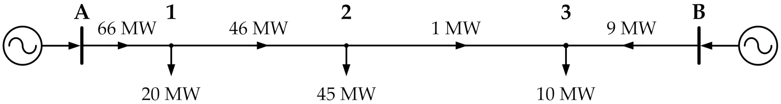
  • the power consumed by the consumer connected to bus 1 (20 MW) flows in its entirety via line A-1 from supply node A,
  • the power consumed by the consumer connected to bus 2 (45 MW) flows in part (25 MW) via lines A-1 and 1-2 from supply node A and in part (20 MW) via lines 2–3 and 3-B from supply node B,
  • the power consumed by the consumer connected to bus 3 (10 MW) flows in its entirety via line 3-B from supply node B.
The results obtained for the analyzed network are presented in Figure 3. Table 3 presents the degrees of individual branch utilization BUb,i by all consumers, resulting from the power flow decomposition by the power flow tracing method. Results were obtained using the Formula (3).
The calculated degrees of individual branch utilization indicate that only the consumer in bus 2 uses all lines, while the consumers in buses 1 and 3 use only the lines connecting them directly to the supply nodes. However, this is not a general conclusion, because in other network operating conditions the situation may be completely different. This difference will occur if the power flow changes.
The voltages in supply nodes A and B were assumed to have the same values in the above calculations. This is a hypothetical situation because the analyzed system is often a part of a larger network, in which the bus voltages result from Kirchhoff’s laws and usually have different values. With a voltage difference between supply nodes A and B, an equalizing power flow will exist between these nodes. This flow will overlap with the natural flow resulting from the loads. As a result, the power flow in the network will change, without changing the values of consumed power. For example, if the equalizing flow between nodes A and B is 21 MW, the value of power flows will change in all lines. Additionally, in line 2-3 the flow direction will change. The new power flow is shown in Figure 4. The change in power flow will also change the degrees of branch utilization by all consumers. Table 4 shows the results.
The above analysis shows that the degree of branch utilization determined by the power flow tracing method strongly depends on the grid operation condition (i.e., depends on the power flow assumed for its calculations). As transmission charges should be based on stable foundations, this dependence on grid operation condition is an unquestionable disadvantage of this method, which makes it difficult to apply in the process of creating a transmission tariff. Therefore, a different method for calculating the degree of network utilization that will be insensitive to changes in power flow is necessary. This requirement is met by the incremental power flow method, based on the superposition principle.

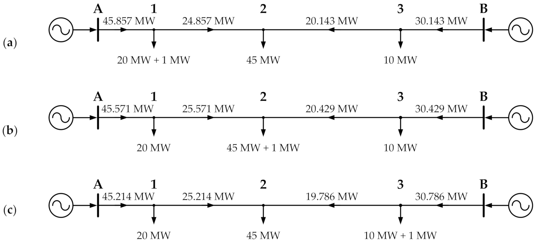
2.3. Power Flow Decomposition by Incremental Power Flow Method

The incremental power flow method is based on the superposition principle. This principle states that, for linear electrical circuits, the resultant response caused by two or more stimuli is the sum of the responses that would have been caused by each stimulus individually. Thus, the natural power flow in the analyzed two-sided supplied network (Figure 2), resulting from the power consumed by all consumers, is the sum of three component flows, calculated using Formula (4) for each consumer separately, with zero powers consumed in other buses. Figure 5 shows these power flows.
The decomposition of base case power flow into three component flows allows for the determining of the degree of branch utilization by individual consumers. The results obtained using the Formula (3) are summarized in Table 5. The calculations consider the directions of power flows for individual consumers (Figure 5) compared to the natural flow (Figure 2). This leads to the appearance of negative values. A negative degree of network utilization could lead to negative values of the transmission charges, which in turn would mean that the network user gains income from the system operator by using the network. To avoid this situation, the degree of network utilization should be determined without considering the differences between the directions of power flows. This approach is used later in the article.
The exact equations defining the power flow are non-linear. To meet the superposition principle, their linearization is necessary, leading to the DC model [20], which is not always suitable for real power systems. Moreover, the use of the superposition principle for power flow decomposition in the real network may cause computational difficulties because, before each calculation of the power flow for a given consumer, the power generated in all sources must be adjusted so that their total generation covers the demand of that consumer. Avoiding these problems is possible with the use of sensitivity factors, that show the impact of the change in power consumed in a given node on the active power flows in the individual network branch [21]. In the considered example of a two-sided supplied network, the values of these factors were determined based on the base case power flow (Figure 2) and power flows calculated after increasing the demand by 1 MW in subsequent load buses (Figure 6). The following formula was used:
S F b , i = Δ P b Δ P i = P b Δ P P b Δ P i ,
where SFb,i is the sensitivity factor of active power flow in branch b with respect to the power consumed in node i, ΔPb is the change of the total active power flow in branch b after increasing the load in node i, ΔPi is the increase of load in node iPi = 1 MW was assumed), P b Δ P is the total active power flow in branch b after increasing the load in node i (Figure 6), and Pb is total active power flow in branch b in a base case (Figure 2). The results of these calculations are summarized in Table 6. A negative value for the sensitivity factor means that increasing the load in a given node reduces the power flow in the branch, comparing to the base case (Figure 2).
The determined sensitivity factors SFb,i can be used to calculate the active power flow in branch b for the consumer in node i, according to the formula [21,22]:
P b , i = S F b , i P i ,
where a negative value means that the calculated power flow for the analyzed consumer has the opposite direction to the base case flow (Figure 2). The application of the Formula (6) and the sensitivity factors presented in Table 6 give the same results for the power flow as that shown in Figure 5, i.e., the degree of individual branch utilization obtained in this way is the same as shown in Table 5.
A characteristic feature of the sensitivity factors is the independence of their values from the power flow. The values of these factors depend on the location of the analyzed node relative to the generators covering the load increase and on the structure and parameters of the network. Thus, for the given structure of the power system and the power consumed in nodes, even for equalizing power flows of any value, the degree of the branch utilization by individual consumers will remain constant. This feature is desirable and it distinguishes this decomposition method from the power flow tracing method. Later in this article, the method of power flow decomposition using the sensitivity factors is called the incremental power flow method.
In the next subsection, the degree of network utilization for the power flow based methods (simple and MW∙km methods) will be defined.

2.4. Definition of the Degree of Network Utilization

In the simple power flow based method, the degree of network utilization is determined by the total flow (TF), defined for the i-th consumer as (definition is based on the idea taken from [5]):
T F i = b P b , i = b S F b , i P i = P i b S F b , i .
In the MW∙km method, the degree of network utilization also considers the length of individual lines (in this article the degree of network utilization calculated by MW∙km method will be called a Total Flow Length–TFL). TFL is defined by the formula [7,9,10,11]:
T F L i = b P b , i l b = b S F b , i l b P i = P i b S F b , i l b ,
where lb denotes the length of line b. The main difference between the degree of network utilization defined by the Formulas (7) and (8) is the fact that the length of lines is not considered in (7). As a result, with the same values of the sensitivity factors SFb,i, lines of different lengths, i.e., with different costs, are treated in the same way. This is a disadvantage of the simple power flow based method, which causes its costs reflectivity to be lower than that of the MW∙km method (Table 1).
The indicated difference between the TF and TFL coefficients can be well-illustrated using the example of a radial network. The network supplies two customers connected as shown in Figure 7. Both customers consume the same power P1 = P2 = P.
In a radial network, the sensitivity factors SF for both consumers are equal to 1. Therefore, TF1 = P and TF2 = 2P, while TFL1 = Pl1 and TFL2 = P(l1 + l2). The transmission charges for both consumers determined from formula (1) will be equal to, respectively:
  • in the simple power flow based method: ⅓ TFC and ⅔ TFC,
  • in the MW∙km method: l1/(2l1 + l2) TFC and (l1 + l2)/(2l1 + l2) TFC,
where TFC is the total fixed cost of the network.
The ratios of charges are as follows: ½ in the simple power flow based method and l1/(l1 + l2) in the MW∙km method. In the first case, this ratio is constant and equal to the quotient of the number of lines involved in supplying consumers (i.e., the first consumer uses one line, and the second one uses two lines). In the second case, the ratio of charges depends on the length of the lines involved in supplying consumers. In an extreme case, e.g., when l1 >> l2, the costs related to the provision of the transmission service for both consumers will effectively be the same. However, in the simple power flow based method, the charge of the first customer, located only slightly closer to the supply point, will be equal to half of the charge of the second customer. In the MW∙km method, these charges will be very similar. Thus, the MW∙km method better reflects the real cost of energy supply.
When determining the degree of network utilization defined by Formulas (7) and (8), three approaches, related to the sign of the sensitivity factor SFb,i, can be used [23]:
  • negative and positive values of SFb,i factors are considered,
  • only positive values of SFb,i factors are considered,
  • absolute values of SFb,i factors are considered.
In this article, the third approach is used, meaning Formulas (7) and (8) can be written as:
T F i = P i b S F b , i ,
T F L i = P i b S F b , i l b .
Using the above Formulas (9) and (10), the degree of network utilization by consumers connected to the simple two-sided supplied network, considered in the previous section, was calculated. The results are summarized in Table 7.

2.5. Practical Aspects of the Calculation of the Sensitivity Factors in the Real Network

The sensitivity factor SFb,i is a derivative that expresses the change in the active power flow Pb in the branch b as a result of the change in the load Pi in node i. Due to the non-linearity of the AC power flow, in practical calculations, the values of these factors are determined based on the results of two power flows: the first one for the increased and the second for the reduced power Pi consumed in the considered bus by the same value of ΔPi. The above can be expressed as:
S F b , i = P b P i P b Δ P P b Δ P 2 Δ P i ,
where P b Δ P and P b Δ P are the calculated active power flows in branch b respectively after increasing and decreasing the load in node i by the value of ΔPi.
When determining the sensitivity factors SFb,i, a key factor is the selection of a generator that will cover the load increments introduced in the analyzed buses. If only one generating node is selected, then the values of the sensitivity factors are calculated with respect to this node. This method can be used when determining the point-to-point charge that is used to settle the transmission costs in a bilateral transaction, i.e., a transaction directly between the consumer and the producer. On the other hand, if the load change is balanced by a group of generators, e.g., by all units that can fully cover the power consumed by a given consumer or by the generators participating in the process of load frequency control, then the values of the sensitivity factors are calculated with respect to all these sources. This way of calculating the sensitivity factors leads to stable values that mainly depend on the existing configuration and electrical parameters of the network. This feature of this method of calculating the transmission charges is highly desirable. Therefore, this article uses a multi-generator approach to cover the load changes.
In the next section, the considered power flow based methods are applied for calculating the rates of fixed transmission charges in the previously analyzed two-sided supplied network. The results of this calculation are compared to the results of the commonly used “postage stamp” method. As an example of practical application, this section also presents a case study for large industrial customers connected to the transmission network

3. The Rates of Fixed Transmission Charges Based on the Degree of Network Utilization

3.1. The Rates of Fixed Transmission Charges in the Two-Sided Supplied Network

The calculated values of the TF and TFL coefficients (Table 7), and the Formula (1), are the basis used to determine the transmission charges for consumers connected to the two-sided supplied network. In the simple power flow based method, the coefficient si in Formula (1) is equal to TFi, while in MW∙km method, it is equal to TFLi. To calculate the “postage stamp” transmission charges, Formula (2) is used. The power consumed by customers connected to the two-sided supplied network (Figure 1) was assumed to be equal to their peak power (Pi = Ppi). By dividing the calculated transmission charges by the peak power of a given consumer, the values of the rates of transmission charges can be obtained.
Both examples in this article present the relative rates of fixed transmission charges, i.e., the rates of transmission charges for a given consumer, determined by each of the analyzed methods, has been referred to the rate of charge calculated using the “postage stamp” method. This is expressed by the formula:
T R i rel . = T F C s i i s i P p i T F C P p i i P p i P p i = s i P p i i s i i P p i ,
where T R i rel . is the relative rate of fixed transmission charge for the i-th consumer. Using Formula (12), the rates of transmission charges can be calculated without knowing the value of the total fixed costs TFC. Figure 8 presents the results for consumers connected to the two-sided supplied network.
The relative rates of transmission charges calculated using the “postage stamp” method are the same for all consumers. This means that each consumer participates equally in covering the total fixed costs of transmission, regardless of their degree of network utilization. On the other hand, in the case of the power flow based methods, differentiation of rates is noticeable. The consumer connected to bus 1 has the lowest rate. This customer receives power mainly through the line A-1 (Figure 5a), which is also the shortest line in the entire network. Thus, this consumer covers primarily the costs of the line A-1 and covers the cost of the other lines to a much lesser extent. A similar situation takes place in the case of the consumer connected to bus 3. This customer receives power mainly through the line 3-B (Figure 5c). However, the ratio of the power flowing through this line to the power flowing to this consumer from the opposite source is smaller than in the case of the first consumer, which results in a relatively higher degree of network utilization, which in turn results in a higher rate of transmission charge. The consumer connected to node 2 has the highest rate. This customer receives power from both sources in a similar proportion (Figure 5b), and therefore this consumer has the highest network utilization, which is reflected in the value of their rate.

3.2. The Rates of Transmission Charges for Industrial Customers Connected to the Transmission Network

The power flow based allocation methods are suitable to calculate the transmission charges for consumers connected to a high and extra-high voltage grids. As an example of practical application, the incremental power flow method was used to determine the rates of fixed charges for large industrial customers connected to the transmission network. The analyzed consumers are characterized by high electricity consumption with relatively low variability in time. Three categories of industrial customers were distinguished:
  • category 1–consumer connected to the 220 kV network node,
  • category 2–consumer connected to the strong 110 kV network node,
  • category 3–consumer connected to the node located deep inside the 110 kV network.
Figure 9 shows an example supply method for consumers belonging to the different categories.
The calculations were made using the model of the Polish power system. This model included the 400 kV and 220 kV networks, owned by the transmission system operator (TSO), and the 110 kV grid, owned by distribution system operators (DSOs). The model reflected the peak load of the Polish power system in 2018 (19.00, February 28,2018). In this operating state:
  • the total system load (including transmission losses) was 26,258 MW,
  • generation of centrally dispatched generating units was 17,605 MW,
  • generation of non-centrally dispatched generating units was 8312 MW,
  • the cross-border exchange was 341 MW (import).
Detailed information is available in [24]. Similar to the previous example, the relative rates of fixed transmission charges are calculated according to Formula (12) for the industrial consumers.
An example of a consumer of category 1 (Figure 9a) is an industrial plant with a peak load of 99 MW. This plant is connected to the 220 kV grid, which means that it uses only the 400 kV and 220 kV networks (consumers of category 1 do not use the 110 kV grid). In this power system operating state, the total load of the 400 kV and 220 kV networks was 14,420 MW. Table 8 shows the degree of network utilization by the example category 1 industrial customer and the total value in the entire 400 kV and 220 kV networks.
The relative rates of transmission charges are 1.27 in the simple power flow based method and 0.46 in the MW∙km method. The difference in the values of the rates can be explained using the data presented in Table 8. Namely, if we divide the TF coefficient for the considered consumer by the power consumed, we will get 368 MW ÷ 99 MW = 3.7. If we do the same for the entire network, we will get 41,801 MW ÷ 14,420 MW = 2.9. The first calculated value can be interpreted as the number of virtual lines involved in the supply of the energy to the analyzed customer, while the second value can be interpreted as an average in the entire network. The ratio of both values is the relative rate of transmission charge for the customer (see Formula (12)). The analyzed consumer uses a greater number of transmission lines than the average for other customers, so the analyzed consumer should pay more for using the network. Therefore, the rate calculated using the simple power flow based method is higher than unity.
Proceeding analogously with the TFL coefficient, the following results are obtained:
  • for the considered consumer: 5855 MW·km ÷ 99 MW = 59.1 km,
  • in the entire network: 1,837,236 MW·km ÷ 14,420 MW = 127.4 km.
The results above can be interpreted as an equivalent transmission distance for the consumer and the average equivalent transmission distance in the entire network. The ratio of calculated values is the relative rate of transmission charge. Since the equivalent transmission distance for the consumer is much shorter than the average for the entire network, the rate calculated using the MW·km method is much lower than unity.
The reason for this large of a discrepancy between the rates determined by the simple power flow based method (1.27) and the MW·km method (0.46) is the means of transmission of the electricity to the considered customer. This consumer is powered by a relatively large number of short lines (shorter than the average line length in the entire 400 kV and 220 kV network). As a result, the degree of network utilization determined by the customer’s TF coefficient is high. Including the length of lines in the TFL coefficient significantly reduces the degree of network utilization. This issue was discussed with a simple example in Section 2.4.
Calculations for customers connected to the 110 kV grid (consumers of categories 2 and 3) were made for two industrial customers supplied from the grids of two different distribution system operators. The 110 kV network of the first operator (DSO 1), which supplies the consumer of category 2 (Figure 9b), is a network with a low area density and relatively long transmission lines. The network of the second operator (DSO 2), to which the consumer of category 3 is connected (Figure 9c), has a higher density with much shorter lines. The total network loads of both DSOs are similar, and equal to 860 MW and 925 MW, respectively. Table 9 shows the degree of network utilization by the considered industrial customers of categories 2 and 3 and the total value in the entire 110 kV networks of both DSOs.
The average number of virtual lines involved in the supply of the energy to the consumers in the entire network is 4 (DSO 1) and 4.6 (DSO 2). The average equivalent transmission distance is 24.2 km (DSO 1) and 16.6 km (DSO 2). The difference in these values is mainly the result of the network density in a given area (a higher density gives a greater number of virtual lines involved in the supply of the energy and a smaller equivalent transmission distance).
For the consumer of category 2 connected to the network of the DSO 1, the number of virtual lines is 1.8 and the equivalent transmission distance is 12.4 km. For the consumer of category 3 connected to the network of the DSO 2, the number of virtual lines is 4.3 and the equivalent transmission distance is 13 km. The differences mainly result from the means of supply for these consumers (Figure 9b,c), but also arises from the network density in the given area.
Figure 10 shows the relative rates of transmission charges for industrial customers for the three different categories. As has already been pointed out, both power flow based methods analyzed in this article give different results for the allocation of fixed costs. For some customers, such as consumers of category 1, these differences can be significant. Considering the previously discussed features of these methods, the MW·km method is recommended.

3.3. Potential Benefits Resulting from the Implementation of the Proposed Methodology in the Energy Market

The transmission charges calculated according to the methodology proposed in this article reflect the costs of utilizing the network more accurately than the charges determined using the currently used “postage stamp” method. As a result of the implementation of these charges on the energy market, new industrial plants can be more often located in places where the transmission costs are lower. Places with low transmission costs are usually close to a power plant. The shorter distance between the generator and the consumer increases the reliability of the power supply due to a smaller number of network elements being necessary for energy transport (the probability of failure of the supply system is lower). The costs of undelivered energy caused by a system failure can be 100 times higher than electricity prices during normal conditions [25]. Therefore, the minimization of these costs is desirable.
Locating consumers closer to power plants will reduce the need to invest in overall network development. As a result, the fixed costs of the network will be lower, and therefore the transmission charges for all groups of consumers will also be lower. Limiting the need for network development will reduce the negative impact of the power sector on the natural environment and conflicts with the local community (protests related to the construction of transmission lines have intensified in recent years). Another benefit of locating industrial consumers closer to power plants will be the reduction of transmission losses. The decrease of losses will reduce emissions related to electricity generation and, furthermore, increase the energy efficiency of the energy supply process. Moreover, the cost of losses, one of the components leading to the variable costs of the network, is now covered by the customers, by using the variable transmission charge. As a result of the lower costs of losses, the charges for all customers will be lower.

4. Summary and Conclusions

The transmission charges should reflect, as fully as possible, the actual costs of supplying energy to individual consumers. These costs depend on which network elements are used and the extent to which they have been used. The current model of calculating transmission charges in Poland, along with other European countries, assumes that the fixed charge paid by a given consumer is proportional to their peak power. This approach is incorrect, and it leads to averaging (socializing) of the costs of providing the transmission service. As a result, there is a cross-subsidization between consumers, i.e., a situation in which some customers generate costs and others are required to cover them.
Various methods can be used to determine which network elements participate and to what extent they participate in supplying the energy to a given consumer. This article focuses on the application of power flow based methods as the most accurate for calculating costs because the power flow in the network is the basic quantity that characterizes its operating condition. The simple power flow based method and the MW·km method were used to define the coefficients determining the degree of network utilization by individual consumers. The degree of network utilization defined by the MW·km method better reflects the cost of supplying energy to a given customer. The advantage of this method comes from considering the length of the line, i.e., the quantity on which the cost of these network elements depends.
To calculate the value of the coefficients determining the degree of network utilization, both the power flow tracing method and the incremental power flow method were examined. The main features of these methods were highlighted using a simple example of a two-sided supplied network. The recommended method is the incremental power flow method, because the calculated degree of network utilization depends mainly on the configuration and electrical parameters of the network branches and the location of the generators. Because the variability of these factors over time is low (the changes in the structure of the network and the location of energy sources result from the construction of new or decommissioning existing facilities), the values of the coefficients will be stable over long periods. For calculating the rates of fixed transmission charges, which are determined for annual or longer periods, this lack of variability is a desirable feature. Additionally, the incremental power flow method considers all potential supply routes to consumers, so it naturally takes into account the reliability of the power supply.
The analyses carried out in a real-world transmission network allowed for the estimation of the rates of a fixed charge for industrial customers characterized by high and stable energy consumption. The practical application of the method discussed in this article would consist in calculating rates for certain categories of customers characterized by similar degrees of network utilization. The charges for each individual customer can also be calculated. Individual charges for industrial customers have recently been implemented in Germany. For this implementation, the shortest supply path method was used. This methodology was approved by the European Commission [26]. Therefore, the method presented in this article is also feasible for practical application, especially as it is consistent with the EU policy, aimed at reflecting in the transmission charges the actual costs of utilizing the network.

Author Contributions

R.K., H.K. and H.M. contributed equally to this work and all of its stages and elements. All authors have read and agreed to the published version of the manuscript.

Funding

This research received no external funding.

Institutional Review Board Statement

Not applicable.

Informed Consent Statement

Not applicable.

Data Availability Statement

Data sharing is not applicable to this article.

Conflicts of Interest

The authors declare no conflict of interest.

Appendix A

This appendix contains a derivation of the Formula (4) that was used to calculate the power flow in a two-sided supplied network shown in Figure A1.
Figure A1. Diagram of a two-sided supplied network.
Energies 14 00614 g0a1
The voltage loss ΔUAB can be calculated from the formula:
Δ U ¯ AB = U ¯ A U ¯ B = 3 I ¯ A 1 Z ¯ A 1 + I ¯ 12 Z ¯ 12 + I ¯ 23 Z ¯ 23 + I ¯ 3 B Z ¯ 3 B ,
where:
I ¯ 12 = I ¯ A 1 I ¯ 1 ,
I ¯ 23 = I ¯ A 1 I ¯ 1 I ¯ 2 ,
I ¯ 23 = I ¯ A 1 I ¯ 1 I ¯ 2 I ¯ 3 .
Considering Formulas (A2)–(A4), Formula (A1) can be written as:
Δ U ¯ AB = 3 I ¯ A 1 ( Z ¯ A 1 + Z ¯ 12 + Z ¯ 23 + Z ¯ 3 B ) I ¯ 1 ( Z ¯ 12 + Z ¯ 23 + Z ¯ 3 B ) I ¯ 2 ( Z ¯ 23 + Z ¯ 3 B ) I ¯ 2 Z ¯ 3 B = = 3 I ¯ A 1 Z ¯ AB ( I ¯ 1 Z ¯ 1 B + I ¯ 2 Z ¯ 2 B + I ¯ 3 Z ¯ 3 B )
from which the current IA1 can be calculated:
I ¯ A 1 = I ¯ 1 Z ¯ 1 B + I ¯ 2 Z ¯ 2 B + I ¯ 3 Z ¯ 3 B Z ¯ AB + U ¯ A U ¯ B 3 Z ¯ AB .
Assuming that UA = U1 = U2 = U3 = UB = U, the power SA1 is equal to:
S ¯ A 1 = 3 U ¯ I ¯ A 1 * = 3 U ¯ I ¯ 1 * Z ¯ 1 B * + I ¯ 2 * Z ¯ 2 B * + I ¯ 3 * Z ¯ 3 B * Z ¯ AB * = S ¯ 1 Z ¯ 1 B * + S ¯ 2 Z ¯ 2 B * + S ¯ 3 Z ¯ 3 B * Z ¯ AB * .
If all lines have the same impedance parameters per kilometer (R’, X’), Formula (A7) takes the form:
S ¯ A 1 = R + j X S ¯ 1 l 1 B + S ¯ 2 l 2 B + S ¯ 3 l 3 B R + j X l A B = S ¯ 1 l 1 B + S ¯ 2 l 2 B + S ¯ 3 l 3 B l A B .
When reactive power is omitted, the Formula (A8) simplifies to the form:
P A 1 = P 1 l 1 B + P 2 l 2 B + P 3 l 3 B l A B = i P i l i B l AB .

References

  1. ENTSO-E Working Group Economic Framework, ENTSO-E Overview of Transmission Tariffs in Europe: Synthesis 2019. June 2019. Available online: https://www.entsoe.eu/publications (accessed on 7 April 2020).
  2. Agency for the Cooperation of Energy Regulators (ACER). Practice Report on Transmission Tariff Methodologies in Europe. December 2019. Available online: https://www.acer.europa.eu (accessed on 17 July 2020).
  3. Council of European Energy Regulators (CEER). Electricity Distribution Network Tariffs CEER Guidelines of Good Practice. January 2017. Available online: https://www.ceer.eu (accessed on 6 April 2020).
  4. Mayadeo, H.; Dharme, A.; Abhyankar, A. Comparison of various Sunk Cost Methods of Transmission Pricing. EasyChair Preprint no. 335; Ver. 2. August 2018. Available online: https://easychair.org (accessed on 15 April 2020).
  5. Xiao, Y.; Wang, X.; Wang, X.; Du, C. Transmission Cost Allocation by Power Tracing Based Equivalent Bilateral Exchanges. CSEE J. Power Energy Syst. 2016, 2, 1–10. [Google Scholar] [CrossRef]
  6. Murali, M.; Kumari, M.S.; Sydulu, M. A Comparison of Fixed Cost Based Transmission Pricing Methods. Electr. Electron. Eng. 2011, 1, 33–41. [Google Scholar] [CrossRef] [Green Version]
  7. Orfanos, G.A.; Tziasiou, G.T.; Georgilakis, P.S.; Hatziargyriou, N.D. Evaluation of transmission pricing methodologies for pool based electricity markets. In Proceedings of the 2011 IEEE Trondheim PowerTech, Trondheim, Norway, 19–23 June 2011. [Google Scholar] [CrossRef]
  8. Lima, D.A.; Padilha–Feltrin, A.; Contreras, J. An overview on network cost allocation methods. Electr. Power Syst. Res. 2009, 79, 750–758. [Google Scholar] [CrossRef] [Green Version]
  9. Krause, T. Evaluation of Transmission Pricing Methods for Liberalized Markets. A Literature Survey; ZTH: Zürich, Switzerland, 2003; Available online: https://www.research-collection.ethz.ch (accessed on 15 April 2020).
  10. Jing, Z.; Duan, X.; Wen, F.; Ni, Y.; Wu, F.F. Review of Transmission Fixed Costs Allocation Methods. In Proceedings of the 2003 IEEE Power Engineering Society General Meeting, Toronto, ON, Canada, 13–17 July 2003. [Google Scholar] [CrossRef] [Green Version]
  11. Venkatesh, P.; Manikandan, B.V.; Charles Raja, S.; Srinivasan, A. Electrical Power Systems Analysis, Security and Deregulation; PHI Learning Pvt. Ltd.: New Delhi, India, 2012; pp. 489–495. [Google Scholar]
  12. Rubio-Oderiz, F.J.; Perez-Arriaga, I.J. Marginal pricing of transmission services: A comparative analysis of network cost allocation methods. IEEE Trans. Power Syst. 2000, 15, 448–454. [Google Scholar] [CrossRef] [Green Version]
  13. Reneses, J.; Rodríguez Ortega, M.P. Distribution pricing: Theoretical principles and practical approaches. IET Gener. Transm. Distrib. 2014, 8, 1645–1655. [Google Scholar] [CrossRef]
  14. Jing, Z.; Wen, F. Review of Cost Based Transmission Losses Allocation Methods. In Proceedings of the 2006 IEEE PES Power Systems Conference and Exposition, Atlanta, GA, USA, 29 October–1 November 2006. [Google Scholar] [CrossRef]
  15. Teng, J.H. Power flow and loss allocation for deregulated transmission systems. Int. J. Electr. Power Energy Syst. 2005, 27, 327–333. [Google Scholar] [CrossRef]
  16. Salgado, R.S.; Moyano, C.F.; Medeiros, A.D.R. Reviewing strategies for active power transmission loss allocation in power pools. Int. J. Electr. Power Energy Syst. 2004, 26, 81–90. [Google Scholar] [CrossRef]
  17. Yang, Z.; Lei, X.; Yu, J.; Lin, J. Objective transmission cost allocation based on marginal usage of power network in spot market. Int. J. Electr. Power Energy Syst. 2020, 118. [Google Scholar] [CrossRef]
  18. Bialek, J. Tracing the flow of electricity. IEE Proc. Gener. Transm. Distrib. 1996, 143, 313–320. [Google Scholar] [CrossRef] [Green Version]
  19. Kirschen, D.; Allan, R.; Strbac, G. Contributions of individual generators to loads and flows. IEEE Trans. Power Syst. 1997, 12, 52–60. [Google Scholar] [CrossRef] [Green Version]
  20. Stott, B.; Jardim, J.; Alsac, O. DC Power Flow Revisited. IEEE Trans. Power Syst. 2009, 24, 1290–1300. [Google Scholar] [CrossRef]
  21. Wood, A.J.; Wollenberg, B.F. Power Generation, Operation and Control, 2nd ed.; John Wiley & Sons Inc.: New York, NY, USA, 1996; pp. 421–424. [Google Scholar]
  22. Hinojosa, V.H.; Gonzalez-Longatt, F. Preventive Security-Constrained DCOPF Formulation Using Power Transmission Distribution Factors and Line Outage Distribution Factors. Energies 2018, 11, 1497. [Google Scholar] [CrossRef] [Green Version]
  23. Lo, K.L.; Hassan, M.Y.; Jovanovic, S. Assessment of MW-mile method for pricing transmission services: A negative flow-sharing approach. IET Gener. Transm. Distrib. 2007, 1, 904–911. [Google Scholar] [CrossRef] [Green Version]
  24. Polish Power System Operation. Available online: https://www.pse.pl/web/pse-eng/data/polish-power-system-operation (accessed on 31 March 2020).
  25. Majchrzak, H. Problems related to balancing peak power on the example of the Polish National Power System. Arch. Electr. Eng. 2017, 66, 207–221. [Google Scholar] [CrossRef]
  26. Commission Decision (EU) 2019/56 of 28 May 2018 on aid scheme SA.34045 (2013/c) (ex 2012/NN) Implemented by Germany for Baseload Consumers under Paragraph 19 StromNEV. Available online: http://data.europa.eu/eli/dec/2019/56/oj (accessed on 10 September 2020).
Figure 1. Diagram of a simple two-sided supplied network.
Energies 14 00614 g001
Figure 2. Natural active power flow in the analyzed network (base case power flow).
Energies 14 00614 g002
Figure 3. Decomposition of the base case power flow by the power flow tracing method–active power flows in the branches for the consumer in the bus: (a) 1; (b) 2; (c) 3.
Energies 14 00614 g003aEnergies 14 00614 g003b
Figure 4. Active power flow in the analyzed network after considering the equalizing flow.
Energies 14 00614 g004
Figure 5. Decomposition of the base case power flow by the superposition principle–active power flows in the branches for the consumer in the bus: (a) 1; (b) 2; (c) 3.
Energies 14 00614 g005
Figure 6. Natural active power flow after increasing the demand by 1 MW in bus: (a) 1; (b) 2; (c) 3.
Energies 14 00614 g006
Figure 7. Radial network supplying two customers consuming the same power.
Energies 14 00614 g007
Figure 8. Relative rates of fixed transmission charges for consumers connected to the two-sided supplied network.
Energies 14 00614 g008
Figure 9. Example supply method of the industrial customers belonging to the different categories. (a) category 1–consumer connected to the 220 kV network node, (b) category 2–consumer connected to the strong 110 kV network node, (c) category 3–consumer connected to the node located deep inside the 110 kV network.
Energies 14 00614 g009
Figure 10. The relative rates of transmission charges for industrial customers of different categories.
Energies 14 00614 g010
Table 1. General assessment of the fulfillment of requirements for the transmission charge for various fixed costs allocation methods.
Allocation MethodCosts ReflectivityPrice SignalsCosts RecoverySimplicity
“Postage stamp”lowlackfullhigh
Power flow based:
Simpleaverageaveragefullaverage
MW∙km (or MW∙mile)goodgoodfullaverage
Marginal costs based:
Short-runvery goodvery goodfulllow
Long-runvery goodvery goodfulllow
Table 2. Major advantages and drawbacks of various fixed costs allocation methods.
Allocation MethodAdvantagesDrawbacks
“Postage stamp”Simplicity:
  • low computational complexity
  • a small amount of data needed
  • easy to understand and apply
Lack of price signals
Cross-subsidization between customers
An equal degree of network utilization is assumed for all consumers
Localization of consumer in the power system is not considered
Power flow basedThe influence of each customer on the network is analyzed
Localization of consumer in the power system is considered
Individual degree of network utilization is calculated (cross-subsidization is eliminated)
Depending on the applied power flow decomposition method, the results may be affected by the choice of reference bus or by the choice of network operating conditions
Marginal costs basedEconomic efficiency (in theory, provides the best cost reflection and correct price signals)Does not ensure the recovery of the total fixed costs of the network (the adjustment of rates is necessary; this adjustment may significantly distort the price signals)
High computational complexity
Table 3. The degrees of individual branch utilization by all consumers, resulting from the power flow decomposition by the power flow tracing method–the base case power flow.
The Consumer in the Bus:The Degree of Branch Utilization
A-11-22-33-B
MW/MW%MW/MW%MW/MW%MW/MW%
120/4544000000
225/455625/2510020/2010020/3067
300000010/3033
Sum45/4510025/2510020/2010030/30100
Table 4. The degrees of individual branch utilization by all consumers, resulting from the power flow decomposition by the power flow tracing method–the equalizing flow considered.
The Consumer in the Bus:The Degree of Branch Utilization
A-11-22-33-B
MW/MW%MW/MW%MW/MW%MW/MW%
120/6630000000
245/666845/46980000
31/6621/4621/11009/9100
Sum66/6610025/2510020/2010030/30100
Table 5. The degrees of individual branch utilization by all consumers, resulting from the power flow decomposition by the superposition principle–the base case power flow.
The Consumer in the Bus:The Degree of Branch Utilization
A-11-22-33-B
MW/MW%MW/MW%MW/MW%MW/MW%
117.14/4538−2.86/25−112.86/20142.86/3010
225.71/455725.71/2510319.29/209619.29/3064
32.15/4552.15/258−2.15/20−107.85/3026
Sum45/4510025/2510020/2010030/30100
Table 6. Sensitivity factors of active power flow in branches with respect to the power consumed in buses.
The Consumer in the Bus:Sensitivity Factors of Active Power Flow in the Branch
A-11-22-33-B
MW/MWMW/MWMW/MWMW/MW
10.857−0.1430.1430.143
20.5710.5710.4290.429
30.2140.214−0.2140.786
Table 7. The degree of network utilization by consumers connected to the two-sided supplied network.
The Consumer in the Bus:TFTFL
MWMW∙km
125.7342.9
290.01542.9
314.3235.7
Sum130.02121.5
Table 8. The peak power and the degree of network utilization by the consumer of category 1.
Consumer and NetworkPpTFTFL
MWMWMW∙km
Consumer of category 1993685,855
Entire 400 kV and 220 kV networks14,42041,8011,837,236
Table 9. The peak power and the degree of network utilization by consumers of categories 2 and 3.
Consumer and NetworkPpTFTFL
MWMWMW∙km
Consumer of category 24480547
Entire 110 kV network of DSO 1860342620,928
Consumer of category 368289885
Entire 110 kV network of DSO 2925425715,344
Publisher’s Note: MDPI stays neutral with regard to jurisdictional claims in published maps and institutional affiliations.

