Abstract
Calculation of fin efficiency is necessary for the design of heat exchangers. This efficiency can be calculated for individual finned tubes or continuous fins. Continuous fins are mostly used in plate-fin and tube heat exchangers (PFTHEs). In most cases, the basic elements of those PFTHEs are circular, oval or flattened pipes, which contain circular or polygonal fins. Continuous fins, as can be observed in PFTHEs, are divided into virtual fins. Those fins can have a rectangular shape for an inline arrangement of pipes or a hexagonal shape for a staggered arrangement of pipes. This research shows a methodology of using the finite element method for calculating the efficiency of fins of any shape, placed on pipes of any shape. This paper presents examples of determining the efficiency of seeming fins, which are most commonly used in PFTHEs. In the article, we also compare the precision of calculations of the efficiency of complex-shaped fins using exact analytical methods and approximated methods: the equivalent circular fin method (Schmidt’s method) and the sector method. The results of the analytical methods and the approximate methods are compared to the results of numerical simulations. The calculations for continuous fins with complicated shapes of virtual fins, e.g., hexagonal elongated or segmented, are also presented.
1. Introduction
Finned surfaces are widely used, e.g., in electronic components, heating, cooling and ventilation systems, power plants and car radiators. The first references for calculating the effectiveness of finned surfaces were described by Harper and Brown [1] in 1922. Up to this point, the calculations of the efficiency of fins with simple and complex shapes have been described several times. Bošnjaković et al. [2] compare the analytical and numerical methods for annular fins. Jing et al. [3] used the calculation of the fin efficiency of a serrated type of finned surface for more complicated research on the air–water heat exchanger for the data center. Nakhchi et al. [4] used the calculation of the effectiveness of stepped fins’ area on the performance improvement of phase change thermal energy storage.
Fin efficiency is described by the ratio of the difference between the average fin temperature and ambient temperature and the difference between the fin base temperature and the ambient temperature. There is a possibility to calculate the exact value of the fin efficiency in the case of simple shapes such as straight or circular fins [5]. However, for complex shapes such as virtual rectangular or virtual hexagonal fins, we must use approximate analytical methods: the Schmidt method (which is less precise, but also less complicated) [6] or the sector method [7]. Moreover, in the case of more complex shapes, e.g., elongated hexagonal or segmented, it is only possible to use numerical methods: the finite element method (FEM) or finite volume method (FVM) [8]. Numerical methods are intended to determine the efficiency of the fin for both simple and complex fin shapes [8]. So far, Osorio et al. [9] analyzed many fin shapes (triangular, square, rectangular, polygonal and trapezoidal) in steady-state using FEM and FVM.
This article presents the comparison of the sector, Schmidt, and numerical methods for fins of standard shape (such as straight or circular) and complex shape (rectangular, hexagonal, elongated hexagonal or segmented). The ANSYS CFX program, which uses the finite volume method, was used to perform a numerical simulation of the efficiency of the fins under heat conduction conditions. For similar problems, the finite element method can also be used, by means of which similar results are obtained for heat conduction problems. Numerical simulations were proceeded by a mesh independent study for all fin shapes. Firstly, the fin end temperature was determined. Stabilization of this temperature meant a sufficiently dense mesh. On this basis, the sizes of mesh elements for numerical simulation were selected, then the efficiency of individual fins was determined. Numerical simulations were conducted for all fin shapes and the following mesh element sizes: 5 × 10⁻⁵ m, 1 × 10⁻⁴ m, 1.5 × 10⁻⁴ m, 2 × 10⁻⁴ m and 3 × 10⁻⁴ m (where the element size is the maximum value of the element’s side). All meshes mainly included quadrilateral elements. The areas of all the fins are similar (the same order of magnitude).
This article presents the following issues:
- Comparison of fin efficiency between analytical and numerical methods for simple fin shapes—straight and circular;
- Comparison of fin efficiency between approximate and numerical methods for complex fin shapes—virtual rectangular and virtual hexagonal (determined from the continuous fin);
- Comparison of fin efficiency between particular numerical simulations for different mesh element size values for complex fin shapes—elongated hexagonally and segmented.
2. Problem Statement
This paper consists of the calculation of fin efficiency under two-dimensional steady-state conditions based on the following assumptions:
- Omission of the radiation effect;
- Omission of the heat transfer from the tip of the fin to the air (Figure 1);
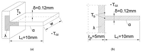 Figure 1. Schemas of the fins of regular geometry: (a) straight fin of constant thickness, (b) circular fin of constant thickness.
 - Omission of the heat transfer on the side if the fin is very thin (assumption: that w >> Lc is satisfied) (Figure 1a);
- Adiabatic boundary condition in the border of the virtual fin designated from the continuous fin because of the fin’s symmetry;
- Constant fin base temperature;
- Constant temperature through the thickness of the fin;
- Constant heat transfer coefficient (α) and thermal conductivity (λ).
The following heat transfer conduction equation (Equation (1)) was designated, taking into account all the above assumptions:
3. Comparing Numerical Simulation Results with Exact Analytical and Approximate Calculations for Determining Fin Efficiency
This research presents methods of establishing the fin efficiency and temperature field in the case of the most commonly used shape of fins. Additionally, the presented methods can also apply to other shapes.
The fin efficiency was calculated for a constant heat transfer coefficient on the fin area using the formula below:
The variable (K) is the average temperature of the fin area. Relative differences between numerical simulation (ηCFD) and analytical and approximate methods were calculated using the formula below:
However, the relative differences formula looks different for elongated hexagonal and segmented fin shapes. The cause of the different formula is the impossibility of carrying out analytical and approximate calculations for ribs with complex shapes.
The thermal parameters used for the calculation were: Tb = 373.15 K, Tcz = 273.15 K and λ = 204 W/(m × K).
3.1. Simple Straight and Circular Fin on a Round Tube
Fins of the straight and circular shape of uniform depth are shown in Figure 1. Those figures present the fin’s dimensions, such as the straight fin’s width (w), the circular fin’s outer radius (rin), the fin’s length (Lc) and the thermal parameters Tcz, Tb, α and λ.
A mesh independent study was carried out for all of the above fin shapes. We can observe that the fin end temperature rose to a stable value of around 363.72 K (Figure 2a) and 359.88 K (Figure 2b). Those stable temperatures mean that the mesh is sufficiently dense and further increasing the number of mesh elements only slightly affects the quality of the result. Moreover, the fin efficiency obtained by the analytical method is very similar to that calculated by the numerical method (Figure 3).
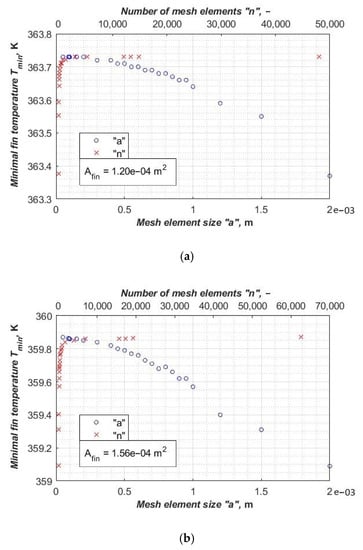
Figure 2.
(a) The minimum fin temperature (for a heat transfer coefficient of 25 W/(m2·K)) as a function of the number ‘n’ of mesh elements and the element size ‘a’ of straight fins. (b) The minimum fin temperature (for a heat transfer coefficient of 25 W/(m2·K)) as a function of the number ‘n’ of mesh elements and the element size ‘a’ of circular fins.
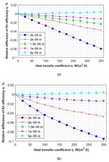
Figure 3.
(a). Relative differences of fin efficiency between numerical and analytical methods for several different mesh sizes as a function of the heat transfer coefficient of the straight fin. (b). Relative differences of fin efficiency between numerical and analytical methods for several different mesh sizes as a function of the heat transfer coefficient of the circular fin.
Figure 3 shows the relative differences between the numerical and analytical results for all of the mesh sizes mentioned above. It can be observed that the results are within the range +0.01%–0.1%, even for the least-dense mesh (element size 3 × 10⁻⁴ m—in the case of this element size, the straight and circular fin meshes consist of 1333 and 1736 elements, respectively). Those results are for the heat transfer coefficient ranging from 0 to 300 W/(m2·K) and for the mesh element size ranging from 3 × 10⁻⁴ m to 5 × 10⁻⁵ m (mesh elements ranging from 1333 to 48,000 elements for the straight fin and from 1736 to 62,512 elements for the circular fin). Additionally, it can be noticed that the relative differences become smaller for the higher number of mesh elements.
It can be noticed that the fin efficiency value for straight and circular fins for the numerical method is very close to the exact analytical result (Figure 4a,b). The fin efficiency (η), as a function of the heat transfer coefficient (α) on the air-side, is presented in Figure 4a for the straight fin and in Figure 4b for the circular fin.
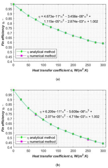
Figure 4.
(a) The fin efficiency (η) as a function of the heat transfer coefficient (α) on the air-side of the straight fin. (b) The fin efficiency (η) as a function of the heat transfer coefficient (α) on the air-side of the circular fin.
3.2. Complex Rectangular and Hexagonal Non-Equilateral Fin on a Round Tube
The main exchangers used in the cross-flow (where heat is exchanged between liquid and gas) are plate-fin and tube heat exchangers. Those heat exchangers consist of tubes and metal sheets. This sheet of metal is called a continuous fin. Simplifications are required to be made in the calculations of plate-fin and tube heat exchangers (PFTHEs) that allow for calculating the efficiency of such fins. The continuous fin was divided into smaller imaginary fins attached to individual pipes (Figure 5).
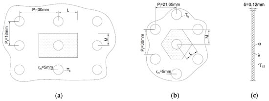
Figure 5.
Virtual fin designation from the continuous fin: (a) rectangular imaginary fin for the parallel pipe arrangement, (b) hexagonal imaginary fin for the staggered pipe arrangement, (c) cross-section of fins (a) and (b).
It can be noticed that the fin’s surface temperature stabilization during the mesh independent study occurred just like in the case of fins with simple geometries. The fin’s minimal temperature stabilized around the temperature of 349.02 K in the case of the rectangular fin (Figure 6a) and 359.84 K in the case of the hexagonal fin (Figure 6b) for the mesh element size of 3 × 10⁻⁴ m. Further increasing the number of mesh elements only slightly affects the quality of the result.
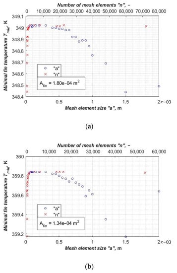
Figure 6.
(a) Fin’s surface minimum temperature (for a heat transfer coefficient of 25 W/(m2·K)) as a function of the number ‘n’ of mesh elements and the element size ‘a’ of the rectangular fin. (b) Fin’s surface minimum temperature (for a heat transfer coefficient of 25 W/(m2·K)) as a function of the number ‘n’ of mesh elements and the element size ‘a’ of the non-equilateral hexagonal fin.
The relative differences comparison of fin efficiency between numerical and approximate methods for five different mesh element sizes is presented in Figure 7 and Figure 8. It can be observed that the relative difference is smaller than 4.00% for the sector (Figure 7) and Schmidt’s (Figure 8) method for mesh element sizes ranging from 3 × 10⁻⁴ m to 5 × 10⁻⁵ m (the number of mesh elements ranging from 2005 to 72,184 for the fin of rectangular shape and from 1491 to 53,672 for the fin of hexagonal shape). The relative differences are similar for both approximate methods. It can be noticed that the accuracy rises as the density of the mesh increases (Figure 7 and Figure 8).
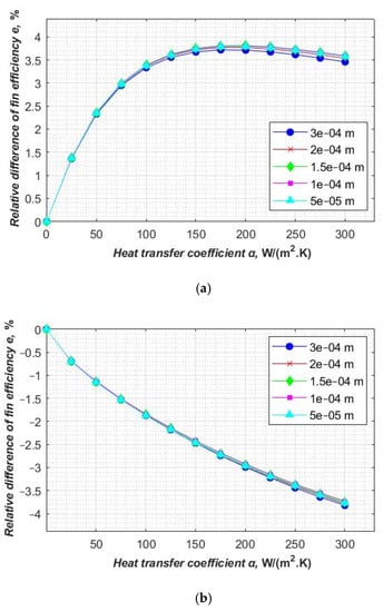
Figure 7.
(a) Relative differences of fin efficiency between the numerical and the approximate sector method in the case of different mesh sizes as a function of the heat transfer coefficient of the rectangular imaginary fin. (b) Relative differences of fin efficiency between the numerical and the approximate sector method in the case of different mesh sizes as a function of the heat transfer coefficient of the non-equilateral hexagonal imaginary fin.
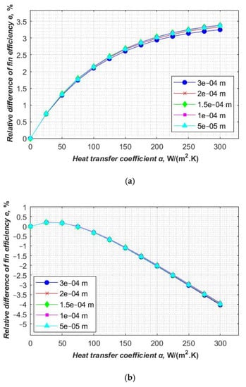
Figure 8.
(a) Relative differences of fin efficiency between the approximate Schmidt’s method and the numerical simulation for several mesh sizes as a function of the heat transfer coefficient of the rectangular imaginary fin. (b) Relative differences of fin efficiency between the approximate Schmidt’s method and the numerical simulation for several mesh sizes as a function of the heat transfer coefficient of the non-equilateral hexagonal imaginary fin.
It can be seen that the fin efficiency value for a rectangular imaginary and non-equilateral hexagonal fin calculated by the numerical method is not very close to the approximate results (Figure 9a,b). The fin efficiency (η) obtained by the numerical method as a function of the heat transfer coefficient (α) on the air-side is presented in Figure 9a for the rectangular imaginary fin and in Figure 9b for the non-equilateral hexagonal imaginary fin.
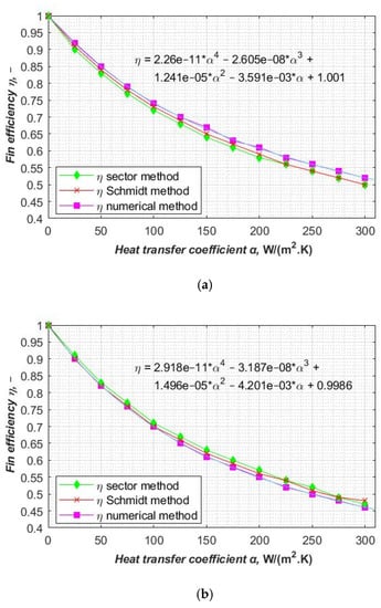
Figure 9.
(a) The fin efficiency (η) as a function of the heat transfer coefficient (α) on the air-side of the rectangular imaginary fin. (b) The fin efficiency (η) as a function of the heat transfer coefficient (α) on the air-side of the non-equilateral hexagonal imaginary fin.
3.3. The Complex Shape of the Fins
3.3.1. The Elongated Hexagonal Fin on a Flat Tube
The numerical method used to determine the fin efficiency and the distribution of temperature may be implemented for any geometry of the fins and be applied to any geometry of the pipes. The numerical simulation’s implementation for the fin efficiency calculation in the case of the imaginary elongated hexagonal shape on flattened pipes is presented in Figure 10. For those types of fins, neither the analytical nor the approximate methods can be used.
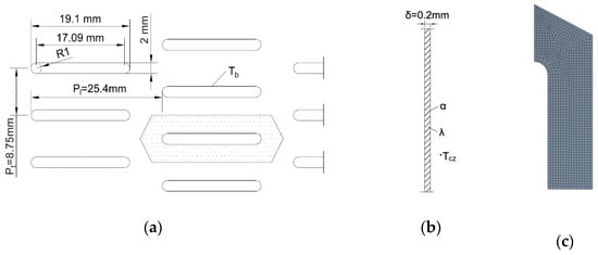
Figure 10.
Plate-finned tube heat exchanger made of flattened pipes with a staggered pipe arrangement: (a) elongated hexagonal imaginary fin for the inline pipe arrangement analyzed in (Thulukkanam, 2013) [10], (b) cross-section of the fin, (c) exemplary division into finite elements for a mesh element size of 3 × 10⁻⁴ m (514 mesh elements).
It can be observed that the fin’s surface temperature stabilization during the mesh independent study is similar in fins with simple and complex geometries. The fin’s minimal temperature has been stabilized around 370.81 K (Figure 11a) for a mesh element size of 3 × 10⁻⁴ m. Further increasing the number of mesh elements only slightly affects the quality of the result. It can be noticed that the relative differences are less than 0.16% for the mesh element size ranging from 3 × 10⁻⁴ m to 5 × 10⁻⁵ m (the number of mesh elements ranging from 514 to 18,494). The four results of independent simulations were slightly different (Figure 11b).
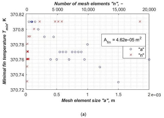
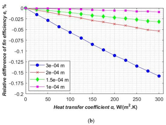
Figure 11.
(a) The minimum fin temperature (for a heat transfer coefficient of 25 W/(m2·K)) as a function of the number of mesh elements and mesh element size. (b) Relative differences of fin efficiency between mesh element sizes 3 × 10⁻⁴ m, 2 × 10⁻⁴ m, 1.5 × 10⁻⁴ m and 1 × 10⁻⁴ m and mesh element size 5 × 10⁻⁵ m.
The fin efficiency (η) for an elongated hexagonal fin for the numerical method is presented in Figure 12. This figure also shows the fin efficiency as a function of the heat transfer coefficient (α) on the air-side.
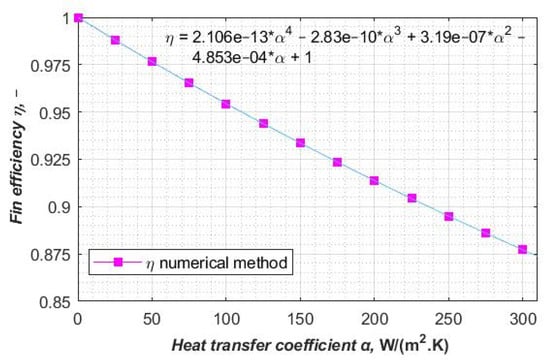
Figure 12.
The fin efficiency (η) as a function of the heat transfer coefficient (α) on the air-side for the elongated hexagonal imaginary fin.
3.3.2. The Complex Segmented Fin on a Round Tube
Figure 13 presents the application of the numerical simulation for calculating the efficiency of the segmented fin on round pipes. Analytical and approximate methods cannot be used for these types of fins. A similar approach was shown in the case of the elongated hexagonal fin in point 3.3.1. However, in this case, fins and pipes are made of boiler steel type P235GH-TC2. The thermal parameters for this steel are: Tb = 373.15 K, Tcz = 1273.15 K and λ = 60.5 W/(m·K). In this case, we took heat from the environment and transferred it to the fin.
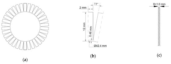
Figure 13.
The complex segmented fins on a round pipe: (a) view of the entire finned tube [10], (b) repeating fin element, (c) cross-section of the fin.
This is the opposite situation to all the previously presented fins, where heat was transferred from the fin to the environment. It should be noticed that the thermal conductivity is less than in previous cases, as described above. That is why the temperature, which stabilizes during the mesh independent study, is falling. In previous cases, the temperature is rising. The fin’s maximum temperature stabilized around 424.56 K (Figure 14a) for the mesh element size of 3 × 10⁻⁴ m. Further increasing the number of mesh elements only slightly affects the quality of the result. It can be noticed that the relative differences are less than 0.035% for the mesh element size ranging from 3 × 10⁻⁴ m to 5 × 10⁻⁵ m (the number of mesh elements ranging from 630 to 23,501). The four results of independent simulations have almost imperceptible differences (Figure 14b).
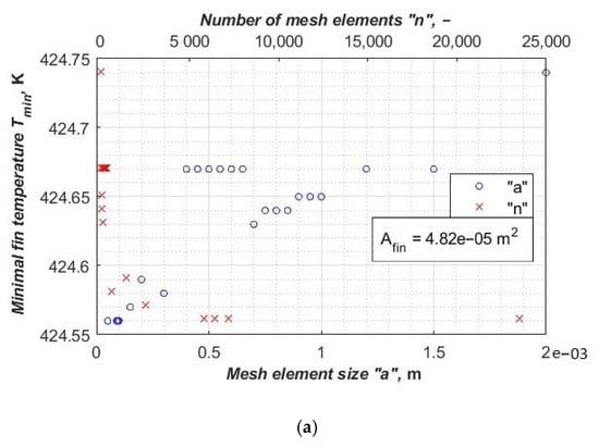
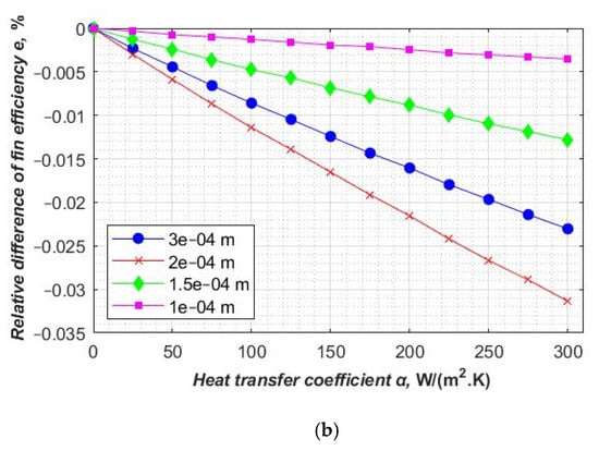
Figure 14.
(a) The minimum fin temperature (for a heat transfer coefficient of 25 W/(m2·K)) as a function of the number of mesh elements. (b) Relative differences of fin efficiency between mesh element sizes 3 × 10⁻⁴ m, 2 × 10⁻⁴ m, 1.5 × 10⁻⁴ m and 1 × 10⁻⁴ m and mesh element size5 × 10−5 m.
The fin efficiency (η) for a segmented fin for the numerical method is presented in Figure 15. This figure also shows the fin efficiency as a function of the heat transfer coefficient (α) on the air-side.
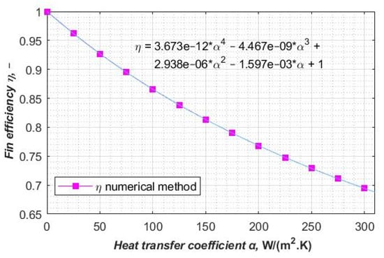
Figure 15.
The fin efficiency (η) as a function of the heat transfer coefficient (α) on the air-side for the segmented fin.
4. Discussion
This paper presents the calculation of fin efficiency by the exact analytical, approximate and numerical methods. It is known that the deviation of thermal performance between experimental and CFD results is less than 4% [11]. Padmanabhan et al. also showed that differences in the temperature distribution between analytical results and CDF analysis are comparable [12]. This paper extends the current state of knowledge about analytical, approximate and numerical results in the case of fin efficiency determination. The comparison’s results in the above article show that the conducted investigation has similar results. This paper presents that the maximum relative differences between the analytical and numerical results are less than 0.1% (Figure 3b). Furthermore, the relative differences between the approximate and numerical results are less than 4.0% (Figure 8b). Fin efficiency in the case of complex geometry can be calculated only by means of numerical simulations. This research shows that numerical results are very precise. The results can be used in further research and industrial fin efficiency calculations. This article does not present considerations about wet or dirty fins, so it could be a natural direction in which to extend this research.
5. Conclusions
Continuous fins can have different geometries, from simple to complex [10]. There are no analytical methods to calculate such fins exactly. Approximate methods are precise, but only for a small range of the heat transfer coefficient α. However, approximate methods are becoming increasingly accurate [13]. All of the above calculations for straight, circular, rectangular, and hexagonal fins demonstrate that numerical methods are very precise and reliable. The simulations were checked by being carried out independently on five types of mesh density.
The comparison of analytical, approximate and numerical methods was presented in this paper. It should be highlighted that all of the above calculations have demonstrated that numerical simulations are reliable. Nevertheless, a mesh element study and suitable validation are needed. The range of the heat transfer coefficient α between 0 to 300 W/(m2·K) was taken into account during the application of all methods. The following conclusions can be drawn from the analysis and calculations performed:
- Relative differences between analytical and numerical simulation results for the mesh element size ranging from 3 × 10⁻⁴ m to 5 × 10⁻⁵ m (the number of mesh elements ranging from 1333 to 48,000) are smaller than 0.1% for 0 ≤ α ≤ 300 W/(m2·K). The results show that we can expect highly precise results from the numerical simulations in the case of complex geometry fins.
- Relative differences between approximate and numerical simulation results for the mesh element size ranging from 3 × 10⁻⁴ m to 5 × 10⁻⁵ m (the number of mesh elements ranging from 514 to 72,184) are smaller than 4.0% for 0 ≤ α ≤ 300 W/(m2·K). This was expected, as approximate methods are not very accurate [8].
- In the case of the most common range in thermal technology, 0 ≤ α ≤ 100 W/(m2·K), relative differences are even more precise than for other values.
- An interesting relationship was noticed during the mesh element studies; the stable minimum temperature and constant fin efficiency occur for the maximum mesh element size of 3 × 10⁻⁴ m (ranging from 514 to 2005 mesh elements) for all presented simulations. Stable values of the fin efficiency changed slightly for a mesh element size between 3 × 10⁻⁴ m and 5 × 10⁻⁵ m (ranging from 514 to 72,184 mesh elements).
- The relative difference does not always increase with an increase in the heat transfer coefficient α.
- The efficiency and speed of current computers, even personal computers, enables very advanced calculations in a relatively short time [14]. The heat conduction simulations presented in the article lasted several seconds for a mesh with 2000–5000 elements. However, for meshes with 50,000–70,000 elements, it took 20–30 s.
Author Contributions
Conceptualization, D.T.; methodology, software, validation, formal analysis, investigation, resources, data curation and writing—original draft preparation, M.M.; writing—review and editing and supervision, D.T. All authors have read and agreed to the published version of the manuscript.
Funding
This research received no external funding.
Data Availability Statement
The data presented in this study are available on request from the corresponding authors.
Acknowledgments
The results presented in this paper were obtained from research work co-financed by the National Science Centre in the framework of the contract STAIR/9/2017—High-performance hybrid solar system for generation of thermal and electrical energy applied for buildings.
Conflicts of Interest
The authors declare no conflict of interest.
Nomenclature
| A | mesh size, m |
| Afin | fin surface area, m2 |
| Lex | fin extended length, m |
| Lc | fin length, m |
| n | number of mesh elements, - |
| Pl | longitudinal fin pitch, m |
| Pt | transversal fin pitch, m |
| rin | outer radius of a plain tube, m |
| T | fin surface local temperature, K |
| Tb | fin base temperature, K |
| Tcz | ambient temperature, K |
| w | fin width, m |
| x, y | cartesian coordinates |
| α | heat transfer coefficient, W/(m2·K) |
| λ | thermal conductivity, W/(m·K) |
| δ | fin thickness, m |
| η | fin efficiency |
References
- Harper, D.R.; Brown, W.B. Mathematical equations for heat conduction in the fins of air cooled engines. NACA R 1922, 158, 32. [Google Scholar]
- Bošnjaković, M.; Muhič, S.; Čikić, A.; Živić, M. How Big Is an Error in the Analytical Calculation of Annular Fin Efficiency? Energies 2019, 12, 1787. [Google Scholar] [CrossRef]
- Jing, H.; Quan, Z.; Zhao, Y.; Wang, L.; Ren, R.; Liu, R. Thermal Performance and Energy Saving Analysis of Indoor Air–Water Heat Exchanger Based on Micro Heat Pipe Array for Data Center. Energies 2020, 13, 393. [Google Scholar] [CrossRef]
- Nakhchi, M.E.; Hatami, M.; Rahmati, M.A. numerical study on the effects of nanoparticles and stair fins on performance improvement of phase change thermal energy storages. Energy 2021, 215, 119112. [Google Scholar] [CrossRef]
- Taler, J.; Duda, P. Solving Direct and Inverse Heat Conduction Problems; Springer: Heidelberg/Berlin, Germany, 2006. [Google Scholar]
- Schmidt, T.E. Heat transfer calculations for extended surfaces. Refrig. Eng. 1949, 351–357. [Google Scholar]
- Shah, R.K.; Sekulić, D.P. Fundamentals of Heat Exchanger Design; John Wiley & Sons: Hoboken, NJ, USA, 2007. [Google Scholar]
- Taler, D.; Taler, J. Steady-state and transient heat transfer through fins of complex geometry. Arch. Thermodyn. 2014, 35, 117–133. [Google Scholar] [CrossRef]
- Osorio, J.D.; Rivera-Alvarez, A.; Ordonez, J.C. Shape optimization of thin flat plate fins with geometries defined by linear piecewise functions. Appl. Therm. Eng. 2017, 112, 572–584. [Google Scholar] [CrossRef]
- Thulukkanam, K. Heat Exchanger Design Handbook, 2nd ed.; CRC Press: Boca Raton, FL, USA, 2013. [Google Scholar]
- Sathe, A.; Sanap, S.; Dingare, S.; Sane, N. Investigation of thermal performance of modified vertical rectangular fin array in free convection using experimental and numerical method. Mater. Today Proc. 2020. [Google Scholar] [CrossRef]
- Padmanabhan, S.; Thiagarajan, S.; Deepan Raj Kumar, A.; Prabhakaran, D.; Raju, M. Investigation of temperature distribution of fin profiles using analytical and CFD analysis. Mater. Today Proc. 2020. [Google Scholar] [CrossRef]
- Suárez, F.; Keegan, S.D.; Mariani, N.J.; Barreto, G.F. A novel one-dimensional model to predict fin efficiency of continuous fin-tube heat exchangers. Appl. Therm. Eng. 2019, 149, 1192–1202. [Google Scholar] [CrossRef]
- Zhai, Z.J.; Zhang, Z.; Zhang, W.; Chen, Q.Y. Evaluation of various turbulence models in predicting airflow and turbulence in enclosed environments by cfd: Part 1—summary of prevalent turbulence models. HVAC R Res. 2020, 13, 853–870. [Google Scholar] [CrossRef]


Publisher’s Note: MDPI stays neutral with regard to jurisdictional claims in published maps and institutional affiliations. |
© 2021 by the authors. Licensee MDPI, Basel, Switzerland. This article is an open access article distributed under the terms and conditions of the Creative Commons Attribution (CC BY) license (http://creativecommons.org/licenses/by/4.0/).