The Effect of Insulation Characteristics on Thermal Instability in HVDC Extruded Cables


Department of Electrical Energy Engineering and Information “Guglielmo Marconi”, University of Bologna, Viale Risorgimento 2, 40136 Bologna, Italy
*
Author to whom correspondence should be addressed.
Energies 2021, 14(3), 550; https://doi.org/10.3390/en14030550
Submission received: 28 December 2020
/
Revised: 13 January 2021
/
Accepted: 16 January 2021
/
Published: 21 January 2021
(This article belongs to the Section F: Electrical Engineering)
Abstract
:This paper aims at studying the effect of cable characteristics on the thermal instability of 320 kV and 500 kV Cross-Linked Polyethylene XLPE-insulated high voltage direct-current (HVDC) cables buried in soil for different values of the applied voltages, by the means of sensitivity analysis of the insulation losses to the electrical conductivity coefficients of temperature and electric field, a and b. It also finds the value of dielectric loss coefficient for DC cables, which allows an analytical calculation of the temperature rise as a function of insulation losses and thermal resistances. A Matlab code is used to iteratively solve Maxwell’s equations and find the electric field distribution, the insulation losses and the temperature rise inside the insulation due to insulation losses of the cable subjected to load cycles according to CIGRÉ Technical Brochure 496. Thermal stability diagrams are found to study the thermal instability and its relationship with the cable ampacity. The results show high dependency of the thermal stability on the electrical conductivity of cable insulating material, as expressed via the conductivity coefficients of temperature and electric field. The effect of insulation thickness on both the insulation losses and the thermal stability is also investigated.
1. Introduction
High voltage direct-current (HVDC) cables have progressively been used in high voltage (HV) transmission systems to meet the increasing energy demand [1]. For the same reason, cable manufacturers are working on innovative materials to withstand higher voltages to meet the increasing demand. So far, HVDC cables have been qualified at rated voltages up to 640 kV [2]. The increase in both the applied voltage and the electric field justifies the need to investigate the insulation losses (i.e., dielectric losses or leakage current losses), which may lead to temperature rise and in some cases to thermal instability (thermal runaway) [3]. In AC cables, insulation losses are caused not only by the leakage (conduction) of current through the dielectric material, but also by dielectric polarization losses—mainly associated with dipolar hysteresis losses—which tend to overwhelm conduction losses. On the contrary, in DC cables, insulation losses are fully driven by leakage current [1].
Intrinsic thermal instability was studied by Whitehead and O’Dwyer [4,5], They worked on thick plane insulations with a constant boundary temperature, which is not fully comparable to this study where the temperature profile is transient according to CIGRÉ Technical Brochure 496 [6] for a cable buried in soil (not a constant boundary temperature). Whitehead found that intrinsic thermal instability occurs at a critical temperature rise (due to only insulation losses) as low as 10 °C [4]. Fallou [7], Brazier [8] and Jeroense and Morshuis [9] studied the so-called “interactive” thermal instability of cables, which occurs in the presence of thermal interaction of the cable with the outer environment. The authors in [9] studied the interactive thermal instability of 450 kV paper-insulated cable and found that the insulation losses become significant for sheath temperatures >70 °C, and interactive thermal instability becomes inevitable for sheath temperatures >83 °C. Eoll first introduced and studied the intrinsic instability of HVDC cables, which can occur even in the absence of thermal interaction with the outer environment [10]. Reddy et al. also studied the intrinsic thermal instability of HVDC cables, considering a 21.7-mm-thick Cross-Linked Polyethylene XLPE-insulated cable at a constant temperature of the metallic screen/sheath, fixed at 25 °C to study the sole effect of the electric field on the thermal stability; the authors calculated the intrinsic Maximum Thermal Voltage (i.e., the maximum DC voltage above which no stability is achieved) and found that interactive Maximum Thermal Voltage will certainly have a lower value. They found out that the critical temperature rise, at which the intrinsic instability takes place, depends almost solely on the insulating material [11].
This paper studies the intrinsic thermal instability—due to the electric field rise or to the effect of cable insulation characteristics—in XLPE-insulated HVDC cables buried in soil. Compared to the above-mentioned papers, the case study tackled here considers a constant interaction of the cable buried in soil having a constant thermal resistivity (neglecting soil drought). Furthermore, the metallic sheath temperature is not constant, as it varies with conductor temperature according to the time variation of applied load current, which involves transient temperature profile. Furthermore, for the sake of completeness and comparison this study considers two different voltage ratings of XLPE-insulated HVDC cables, 320 kV and 500 kV, which involve different insulation thicknesses, so as to analyze the effect of different cable insulation designs.
Thermal stability is investigated from two intrinsic perspectives:
- The insulation material characteristics, focusing here on the electrical conductivity coefficients of both temperature and electrical stress, a and b, respectively.
- The electric field variation as a result of the applied voltage variation. This might happen during testing at very high and/or increasing voltage levels, e.g., during thermal stability tests [12].
This paper also aims at finding the critical values of the conductivity coefficients which guarantee a thermally stable operation of the cable under different applied voltages (and, in turn, in different electric fields).
2. Theoretical Background
2.1. Temperature Profile and Electric Field Calculation
The algorithm followed in this paper depends on an iterative method of electric field calculation and reliability estimation of HVDC cables subjected to load cycles according to CIGRÉ Technical Brochure 496 [6]. It was first developed by Mazzanti by developing a reliability estimation model of HVDC cables subjected to prequalification test (PQ) considering a steady state electric field as a simplification [13], then it was improved to include the transient electric field calculation in [14] instead of the steady state electric field. Later in [15], it was improved to include the type test (TT) load cycles in the algorithm. In [3], the algorithm was improved to consider the temperature rise due to insulation losses.
In this paper, possible thermal instability conditions of both 320 and 500 kV XLPE-insulated HVDC cables are investigated as a function of cable insulation characteristics, represented by the temperature and stress coefficients (a, b) of electrical conductivity of the extruded dielectric and the insulation thickness. The effects of these parameters on temperature rise due to insulation losses and, consequently, on the thermal instability are assessed. The flow chart presented in Figure 1 explains step by step the algorithm implemented for such assessment. First, the temperature profile of load cycles according to CIGRÉ Technical Brochure 496 [6] is calculated using the CIGRE transient thermal network model following the guidelines of Standard IEC 60853-2 [16] (for more details, see [13,14]). Then, the transient electric field inside the insulation of the cable subjected to load cycles is calculated using both Maxwell’s Equations (1)–(3) and conductivity Equation (4) as mentioned in detail in [15], followed by the calculation of insulation losses and the resulting temperature rise. Finally, the thermal stability diagram is found for both studied cables.
Gauss law
Current continuity
Ohm’s law
Conductivity
where E is the electric field vector [], is the vacuum permittivity, is the relative permittivity of the insulation, J is the direct conduction current density vector [], is the free charges density [], σ is the electrical conductivity of the insulation [], is the value of σ at 0 °C and for an electric field equal to 0 kV/mm. As far as electrical conductivity σ is concerned, it should be pointed out that the empirical model suggested by Klein [17] has been used in this paper, as well as in the early stages of this research project, as given by Equation (4), where: is the value of at 0 °C and for an electric field equal to ≈0 kV/mm, a is the temperature coefficient of electrical conductivity (1/K or 1/°C), b is the stress coefficient of electrical conductivity (mm/kV, or m/MV).
2.2. Calculation of Insulation Losses
The temperature rise in the insulation can be found by solving the heat transfer Equation (5) in cylindrical coordinates in the steady-state form ():
where r is the generic radial coordinate in cable insulation, is the thermal resistivity of the insulation, T is the temperature, is the per unit volume power generated due to insulation losses; it represents the source term in the equation and can be found as follows:
where J is the current density inside the insulation, A is the lateral surface area of one meter length of the cylindrical cable at a generic radius r (see Figure 2), and σ is the electrical conductivity of the insulation at the radial coordinate r.
By manipulating (5), one gets:
where the negative Right-Hand Side RHS refers to the reduction of temperature in the direction of which the finite difference method (FDM) is used to solve (7), namely, the temperature variation from the inner-insulation towards the outer-insulation is always a temperature drop. The total dielectric losses in the unit length of cable insulation can be obtained using the following equation, which is derived by integrating (6) in cylindrical coordinates:
As a result of the discretization in r axis, the electrical conductivity is considered constant within the infinitesimal differences dr. Consequently, Equation (8) can be simplified to an integrable form in each infinitesimal interval , as follows:
Boundary conditions:
- Inner boundary conditions: Neumann boundary conditions are applied to the inner insulation near the conductor surface. The RHS of (10) refers to the heat flowing from the conductor to the insulation due to conductor losses in the r axis where the temperature drop takes place.where T1 and T2 are the temperatures at the first and second points of the mesh in the inner insulation.
- Outer boundary conditions: Neumann boundary conditions are applied to the outer insulation, where the heat flow in the direction of the r axis consists of both the heat generated due to conductor losses and the heat generated due to insulation losses. A ghost point n + 1 is placed at the metallic/screen sheath whose temperature is calculated using (13). This gives a more realistic simulation of heat flow in the thermoplastic sheath (which, contrary to the metallic sheath, has a non-negligible thermal resistance [18]) and in the surrounding soil resulting in a more realistic metallic sheath temperature (see both Appendix A and Appendix B).where is the thermal resistance of the thermoplastic sheath, is the thermal resistance of the surrounding soil.
2.3. Calculation of Dielectric Loss Coefficient
The temperature drop in the insulation, thermoplastic sheath and soil can be given by the following equation, (see Figure 3):
where are the temperature drop in the insulation, thermoplastic sheath and soil, respectively, due to both conductor losses and dielectric (or insulation) losses . According to IEC Standard 60287, Equation (14) can be re-written as in (15) [18]:
where: is the temperature drop over the whole cable and soil layers due only to the conductor losses, is the temperature drop over the whole cable and soil layers due only to the insulation losses, and is the dielectric loss coefficient.
By manipulating (15), one obtains the following Equation (16) which is used to calculate the dielectric loss coefficient of DC cable insulation:
By calculating , the temperature drops in the insulation, sheath and soil, due to both conductor and insulation losses, can be found using (17)–(19), respectively:
where is the conductor’s current [A], is the DC electrical resistance of the conductor operating at the temperature , as follows:
where is the temperature coefficient of the electrical resistivity of the conductor at 20 °C.
2.4. Calculation of De-Rating Factor
Since the load current and its heat flow inside the insulation play an important role in the stability of HVDC cables, the calculation of the de-rating factor is needed to accurately define the stability limits. The power generated by the conductor current per meter cable is given by (21):
Accordingly, the de-rating factor can be calculated using (22):
where [W/m] are conductor losses per meter cable at the rated current [A], are the insulation losses per meter cable [W/m], [A] is the de-rated conductor current equivalent to the conductor losses considering insulation losses [W/m].
2.5. Thermal Stability
The stability study can be carried out using the so-called thermal stability diagram (Figure 4). The diagram consists of two basic curves:
- The heat generation curve (red solid curve in Figure 4) refers to the heat generated within the cable due to both insulation losses and conductor losses .
- The heat dissipation line (blue solid line in Figure 4) refers to the heat dissipated outside the cable through the insulation, thermoplastic sheath and soil, . This full straight line is defined using two parameters:
- (1)
- The thermal resistance of the insulation, thermoplastic sheath and soil, represented by the reciprocal of the slope of the dissipation line. The higher the thermal resistance, the lower the slope, resulting in a higher temperature w.r.t the same losses, see dashed blue line in Figure 4;
- (2)
- The ambient temperature, the intersection of the dissipation line with the temperature axis. As the ambient temperature rises, the dissipation line shifts in the direction of the temperature rise without variation in the slope, see dash-dotted blue line in Figure 4.
Thermal instability occurs when thermal equilibrium cannot be achieved. A stable thermal equilibrium is reached only when the total heat of both conductor and insulation losses is equal to the heat dissipated from the cable [8]. This condition is shown in Figure 4 by point (A), the first intersection between the generation curve and the dissipation line. Two cases of thermal instability were introduced in [19]:
where stands for the total losses [W/m], is the heat dissipation [W/m]. The second case of thermal instability refers to the so-called “unstable equilibrium” in which an equilibrium exists but even a slight temperature rise leads eventually to instability. The latter is shown in Figure 4 by point (B).
Thermal instability is of two types:
- Intrinsic thermal instability:
In intrinsic thermal instability, there is no external interaction with the cable, namely no interaction between the cable layers and the outer environment. This type of instability depends on the characteristics of the insulation (dielectric material and insulation thickness) and on the electric field, regardless of the external thermal resistance variation. This type of instability is not associated with a runaway increase in the temperature of the metallic sheath (which in practice coincides with the temperature in the outer insulation surface, since the thermal resistance of the metallic sheath is negligible, see Section 2.2.) unlike the interactive instability [10]. Thus, it occurs even at ambient temperature in the case of unloaded cable [11].
Referring to Figure 4, it can be said that intrinsic thermal instability corresponds to shifting the red curve upwards until an intersection with the blue curve—namely thermal equilibrium—cannot be achieved anymore, even by moving the operating point along the red curve to the right.
- 2.
- Interactive thermal instability:
In interactive thermal instability, an interaction between the cable and the ambient leads to runaway if the equilibrium cannot be reached. In this type of instability, variation of external thermal resistance or variation in the ambient temperature are necessary for the runaway to take place [11]. Referring to Figure 4, it can be said that interactive thermal instability corresponds to shifting the blue curve to the right and/or tilting it downward until the equilibrium (intersection with the solid blue curve) cannot be achieved anymore. Indeed, Figure 4 shows that:
- (i)
- for a value of the ambient temperature ≥Ta2 (dash-dotted line), equilibrium cannot occur, and thermal instability takes place;
- (ii)
- the increase in the thermal resistance of the surrounding soil (dashed line) leads to inevitable thermal instability because the equilibrium cannot exist.
Both intrinsic and interactive instability terminate with the same failure mechanism, which includes an extreme variation in the temperature distribution inside the insulation leading to an extreme rise of the electric field to values greater than the intrinsic dielectric strength of the insulation, and eventually the breakdown occurs [10].
3. Case Study
3.1. Cable Characteristics
3.2. Temperature Profile Calculations
The temperature profiles within the insulation of the 320 kV and 500 kV HVDC cable are calculated for the 24-h load cycles mentioned in CIGRÉ Technical Brochure 496 [6] and prescribed during prequalification tests and type tests (see Figure 5). It is worth recalling briefly that the 24-h load cycles prescribed in [6] consist of at least 8 h of heating followed by at least 16 h of natural cooling, during at least the last 2 h of the heating period, a conductor temperature ≥ rated conductor temperature and a temperature drop across the insulation ≥ rated temperature drop shall be maintained. The insulation thickness is divided by n = 50 points into 49 layers which have a thickness each. The time step is set to be 1 [s] that is found to achieve the stability of the algorithm especially for high values of the electric field and the conductivity.
3.3. Temperature and Stress Coefficients of Electrical Conductivity a, b
Many empirical models have been introduced in the literature to represent the relationship between electrical conductivity and both temperature and electric stress variations for different types of insulation [21,22]. However, as pointed out above, the empirical model suggested by Klein [17] has been used in this paper (see Equation (4)). As far as this model is concerned, many values of conductivity coefficients a, b can be found in literature [21,22,23,24]; however, the set of values reported in [21] is considered in this study (see Table 3), of which the medium set of values corresponds to the XLPE, the low set of values corresponds to paper insulations and the high set corresponds to thermoplastic insulations.
Focusing on thermoset extruded dielectrics for HVDC cables, to which the XLPE insulation of the treated cables belong, let us take the medium set of values of conductivity coefficients aM = 0.084 1/°C, bM = 0.0645 mm/kV as a reference. Due to the high sensitivity of the conductivity to a, b coefficients, more extreme values of a, b—which may fit future insulations—are considered in this study, by taking the medium set of values aM, bM as the base set (multiplier M = 1) and multiplying them by proper values of the multiplier M, as shown in Table 4. In more detail:
- -
- An extremely low set, aL, bL, is obtained by multiplying aM, bM by M = 0.5;
- -
- An extremely high set, aVH, bVH, is obtained by multiplying aM, bM by M = 2;
- -
- The interval [aL, bL ÷ aVH, bVH] is divided into 16 equally distributed sets of a, b values, each identified in Table 4 by the corresponding value of the multiplier M of the medium set aM, bM.
4. Results
4.1. Electric Field Distribution
Figure 6 presents the electric field distribution inside the insulation for both 320 kV cable (Figure 6a) and 500 kV cable (Figure 6b) during the first 24-h load cycle of the load cycle period according to CIGRÉ Technical Brochure 496 [6] (the number of 24-h load cycles of the load cycle period prescribed in [6] is 160 during prequalification tests, 24 during type tests) at a voltage equal to rated voltage U0. This means that the electric field distribution at the first instant is a capacitive distribution. The DC electric field distribution for the cold cable is presented in the blue curve (24 h curve).
In the simulations, different voltages—up to 4.5 times the rated voltage—are applied to the 320 kV XLPE-insulated cable, thereby obtaining the profiles within cable insulation of electric field, electrical conductivity and leakage current, shown in Figure 7, Figure 8 and Figure 9, respectively.
In more detail, Figure 7 presents the DC electric field profiles for (a) the cold cable at ambient temperature, (b) the hot cable (i.e., rated current flowing in the conductor, as prescribed in CIGRÉ Technical Brochure 496 for the 24-h load cycles of the high load period). The maximum mean electric field is ≈80 kV/mm in case of applied voltage = 4.5 U0; the electric field inversion phenomenon is observed in the hot cable (Figure 7b). Figure 8 demonstrates the effect of the applied voltage and temperature on the electrical conductivity in the insulation: it can be seen that the conductivity varies by [1.4 ÷ 2] orders of magnitude between the cold cable (Figure 8a) and the hot cable (Figure 8b). Moreover, it is worth noting that the conductivity of the inner insulation is much greater than that of the outer insulation for the hot cable due to the high temperature of the conductor. This difference in conductivity distribution inside the insulation is lesser in the cold cable because in this case the temperature is constant over the insulation and the quasi-capacitive electric field is the only variable quantity in (4). Figure 8 also illustrates the effect of the applied voltage (i.e., the electric field) on the conductivity of XLPE insulation, which rises by ≈1.5 orders of magnitude when rising the voltage from U0 to 4.5 U0. Figure 9 presents the leakage current for 320 kV XLPE-insulated cable for the considered applied voltages during the first 24-h load cycle of the load cycle period according to CIGRÉ Technical Brochure 496 [6]. It is clear that the leakage current increases by ≈2.5 orders of magnitude by applying 4.5 U0.
4.2. Insulation Losses
Figure 10 shows the insulation losses during the first 24-h load cycle of the load cycle period after [6] compared to the conductor losses in both linear and logarithmic y-scale for both the 320 kV and 500 kV cables subjected to many values of the applied voltage starting from U0, 1.45 U0 and 1.85 U0, which correspond, respectively, to the rated voltage, pre-qualification test (PQT) voltage and type test voltage (TT) according to [6]. It can be seen from Figure 10 that the insulation losses at rated voltage U0, PQT voltage = 1.45 U0 and TT voltage = 1.85 U0 are hardly noticeable compared to conductor losses, having maximum values of (0.06, 0.2, 0.6 W), respectively, which can be deemed negligible compared to the conductor losses ≈ 40 W. Although TT voltage is the most severe condition to be continuously applied on the cable, higher values of the applied voltage are also considered to reach high enough values of insulation losses to cause thermal instability. It is evident that the insulation losses of the 500 kV cable are approximately 1.5 times greater than that of the 320 kV cable (the same as the ratio between their insulation thicknesses). Therefore, the thicker the insulation is, the greater the insulation losses are. This ratio may be different according to the cable’s temperature and time during the load cycle, namely, this can be justified by the field inversion phenomenon which takes place in DC cables, during which the electric field in the outer insulation becomes greater than that in the inner insulation.
4.3. Temperature Rise
Many runs of the code have been performed to obtain the temperature rise in the insulation of the hot cable (i.e., with rated current flowing in the conductor, see above) due to insulation losses—calculated according to Equations (6)–(13)—added to conductor losses. As a further verification, the results obtained have been also checked by calculating—in alternative to (6)—per unit dielectric losses as wd = E2 and the results have been found to be the same. Different values of a, b coefficients are considered to show the effect of the cable characteristics on the insulation losses and consequently on the temperature rise.
It can be noticed from Figure 11 that the temperature rise due to insulation losses is strongly dependent on the values of conductivity coefficients of temperature and electric field for the 320 kV cable. In Figure 11a the low values of a, b (aL, bL) lead to weak dependency of the conductivity on the temperature and the electric field giving a temperature rise of 0.5 [°C] which is not enough for thermal runaway to take place. Figure 11b shows the case of aM, bM, where a considerable temperature rise due to insulation losses can be noticed; the temperature rise is negligible for rated voltage, PQT voltage and TT voltage, it increases by ≈( ÷ 3) °C for 2.5 U0 and thereafter exponentially increases exceeding 30 °C for 4U0. Figure 11c shows the case of the high set aH, bH, in which even a moderate increase of the applied voltage with respect to U0 (e.g., PQT and TT voltages) leads to a temperature rise of [1 ÷ 3] °C; the temperature rise becomes ≈10 °C for an applied voltage equal to 2.5 U0, namely more than three times than in the case of aM, bM.
Coming to the 500 kV cable in case of aM, bM—a set of conductivity coefficients which fits well on the average the overall behavior to XLPE insulating materials—in Figure 12 it can be noticed that the temperature rise is greater than that of the 320 kV cable, due to the greater insulation thickness—since the electric field and the conductor temperature are similar in both cables.
4.4. Calculation of
Figure 13 shows the values of for the 320 kV cable, obtained using relationship (16) calculated at each time step during the first 24-h load cycle of the load cycle period after [6]. Similar curves are obtained for all values of applied voltages, all sets of a and b coefficients, as well as for the 500 kV cable. The capacitive electric field distribution at the beginning of the first load cycle gives a value of , which agrees with the value of mentioned in IEC 60853-2 for AC cables [16]. Then, it goes down within 30 min to fall within the range which represents the typical range of values of for DC cables. As explained here below, this result is consistent with the well-known fact that the electric field of inner insulation in DC is lower than that in AC: this already holds for the unloaded cable (compare in Figure 6 the black curve = AC electric field vs. the blue curve = DC electric field at ambient temperature), but it holds a fortiori as the cable is loaded (see warmer color curves in Figure 6, corresponding to higher cable load and temperature).
Thus, compared to AC cables, the insulation losses in DC cables move towards the outer insulation, i.e., they are lower in the inner insulation and higher in the outer insulation, as readily seen from the alternative expression of per unit volume dielectric losses derived from (3), (6)
(for the loaded cable at outer insulation the quadratic increase in losses due to the higher electric field overwhelms the decrease in losses due to the slight conductivity drop because of lower temperature). Now, by carefully inspecting Equations (15) and (16) it can be understood that, physically, parameter represents the “equivalent”—from the viewpoint of the overall temperature drop across insulation —fraction of dielectric losses crossing the whole thermal resistance of the insulation: as a consequence it is reasonable that is lower in DC than in AC, as dielectric losses in DC cables move towards outer insulation (see above).
4.5. Thermal Stability Diagram
Figure 14 is the so-called “thermal stability diagram” of the 320 kV (Figure 14a) and of the 500 kV (Figure 14b) cables for different values of applied voltage: with reference to Equations (23) and (24), it shows the insulation losses (colored curves) and the dissipation losses (black straight line) on the y-axis as a function of the metallic sheath temperature Tsheath on the x-axis. The metallic sheath temperature in turn varies with conductor temperature according to the term in (15). From this diagram the so-called maximum thermal voltage (MTV) can be attained, namely the maximum value of the applied DC voltage above which no equilibrium is achieved in the design conditions of the environment. For both 320 kV and 500 kV XLPE-insulated cables, the medium set of conductivity coefficients (aM, bM) is considered for the sake of brevity.
Figure 14 shows that the higher the applied voltage, the higher the insulation losses, which reduces the maximum (or critical) value of cable current Icrit that keeps the cable thermally stable. Icrit is obtained from the value of losses found on the y-axis as a complement of the insulation losses to the dissipation line. This implies a reduction in cable load current from the rated current in the design conditions of the environment, ID (cable ampacity), to critical current Icrit: such a load reduction is necessary to avoid thermal instability.
Let us focus for the sake of illustration on Figure 14a: for instance, in the absence of dielectric losses a metallic sheath temperature of 50 °C corresponds to a conductor temperature of 62.5 °C, as obtained from Equation (15) without insulation losses and for a conductor current lower than cable ampacity (note that conductor temperature in the absence of dielectric losses reaches 70 °C when conductor current is equal to cable ampacity and metallic sheath temperature is equal to 55 °C, see Figure 5a). In the case of applied voltage equal to 3.5 times the rated voltage = 1120 kV, the insulation losses are equal to 8.4 W (see point A in Figure 14a) and lead to temperature rise of 8.5 °C in the inner insulation (again from Equation (15)). Then, as pointed out above, the critical value of cable current Icrit can be derived from the vertical distance along y-axis from the dissipation line (see point B in Figure 14a), which is ≈26 W and corresponds to a conductor temperature of 52 °C in the absence of insulation losses. However, this case falls within the “unstable equilibrium” expressed by conditions (24); namely, an equilibrium exists, but even a slight temperature rise leads eventually to instability, unless the cable is further underloaded.
For low applied voltages, in which two equilibrium points can be found, both conditions (24) need to be satisfied to reach the instability. In other words, to ensure thermal stability, a stable equilibrium must exist . Figure 14a shows that a stable thermal equilibrium exists up to 3U0 ≈ 1000 kV (54 kV/mm)—among the considered values of the applied voltages—for a fully loaded (i.e., conductor current equal to cable ampacity) 320 kV XLPE cable buried in soil. When higher voltages are applied, conductor current has to be progressively reduced w.r.t. cable ampacity to keep the cable thermally stable, until conductor current reaches zero at 4.5U0. Thus, in unloaded cable subjected to 4.5U0 no equilibrium between the insulation losses and the heat dissipation exists and thermal instability eventually occurs starting from a temperature rise equal to only 5 °C, then, raising the metallic sheath temperature and moving the operating point towards the direction of the metallic sheath temperature rise (to the right here) until an intersection between the generation curve and the dissipation line exists, if any. Otherwise, thermal instability will be inevitable as occurs anyway in case of 4.5U0, which is the first case of thermal instability (23).
Coming now to Figure 14b—the same as Figure 14a but for the 500 kV cable (aM, bM)—the thermal runaway of intrinsic nature occurs at voltages slightly greater than 4.5U0 ≈ 2250 kV, although the mean electric field necessary to reach thermal instability in unloaded cable is almost the same in both cables having different thicknesses. For lower voltages [2.5 ÷ 4] U0, it can be noticed from Figure 14b that the insulation losses are greater than those of the 320 kV cable at the same voltages, with a more significant exponential rise. This implies more load reduction is required to avoid thermal instability, thus, worsening the stability and loading conditions.
Figure 14b shows that a stable thermal equilibrium exists up to 2.5U0 = 1250 kV (45 kV/mm)—among the considered values of the applied voltages—for a fully loaded 500 kV XLPE cable buried in soil. Thus, this voltage value can be deemed as the maximum thermal voltage of these cables.
4.6. Thermal Instability for Different Cable Characteristics and Applied Voltages
For the sake of the generality of the obtained results, the results for different electrical conductivity characteristics of cable insulation are obtained as can be seen in Figure 15, which shows the insulation losses as a function of mean electric field in the insulation over a wide range of values of mean electric field (from the rated one up to 100 kV/mm) for different a, b coefficients (see Table 4) at the maximum conductor losses (full load) for the 320 kV cable. This figure highlights the importance of the insulating material, represented here by the temperature and electric stress coefficients of electrical conductivity, on the thermal stability of the cable. The very high a, b coefficients give rise to very high insulation losses compared to conductor losses. Some thermoplastic materials tend to have a, b coefficients up to 0.15, 0.128, respectively, which is referred to as M = 1.8 in Figure 15 and Table 4. According to the simulations summarized in Figure 15, materials having such characteristics would not have acceptable thermal stability properties for the insulation of HVDC cables. For materials having the so-called “high” values of a, b coefficients, namely aH, bH with M = 1.2 in Table 4, the insulation losses are low up to TT voltage = 1.85 U0, then they exponentially increase for greater electric fields. Coming to the medium set of a, b coefficients, taken as a reference (M = 1 in Table 4) since they correspond to typical XLPE insulation for HVDC cables [21], it leads to a more stable behavior with low insulation losses up to E = 40 kV/mm which is a conservative value and greater than the electric field in case of type test at 1.85 U0 (the most severe DC voltage to be continuously applied to the cable in tests after [6]). For higher values of the electric field corresponding to a voltage up to 3U0, the insulation losses increase, however, a stable equilibrium can be attained; both stable and unstable equilibrium can be reached for voltages greater than 3U0 (according to loading conditions); but instability becomes inevitable for field values corresponding to a voltage equal to or higher than 4.5U0 (as discussed in Section 4.5). The lower set of values of a, b (M = 0.8, 0.9) which are typical of paper insulations [21] make the intrinsic thermal instability unlikely to take place even for high values of the electric field, say, higher than ≈70 kV/mm. The lowest set of values of a, b coefficients (which, to the best of the authors’ knowledge, does not correspond to any known insulating material used in HVDC applications, but is considered here for the sensitivity analysis), it does not give an insulation loss temperature rise greater than 6 °C for the highest electric field considered in this study.
4.7. De-Rating Factor
Figure 16 demonstrates the de-rated conductor current, the so-called in (22), (Figure 16a) and the de-rating factor, DF in (22), (Figure 16b) w.r.t the applied voltage ranging from U0 to 3 U0. Greater voltages are not studied since 3.5U0 or higher voltages lead to unstable equilibrium at losses equivalent to the rated current as discussed in Section 4.5 and shown in Figure 14. Figure 16 shows that at the rated voltage DF = 1, DF becomes lower than 0.99 at ≈1.8 U0 and then it drops dramatically until the voltage 3U0 where it reaches a value DF = 0.93 for 320 kV cable and DF = 0.88 for 500 kV cable. The results also clearly show that the 500 kV cable is more de-rated than the 320 kV cable for the same applied voltage.
5. Discussion
For the 320 kV cable, the 4.5U0 ≈ 1400 kV curve in Figure 14a refers to thermal instability of an intrinsic nature: no load current is required for instability to take place because of the extreme temperature rise inside the insulation without temperature runaway near the metallic sheath; in this case, the instability occurs even at the ambient temperature, because the insulation losses are enough to heat up the insulation and move the operating point towards higher temperatures (towards right on the red curve Figure 14) until the breakdown occurs due to the absence of any type of equilibrium.
The insulation losses which lead to thermal instability can be found from Figure 14, then the resulting temperature rise is calculated from (15) considering the value of to obtain at . This study shows that thermal instability occurrence is possible even at lower applied voltages because of its dependency on the load current. This value is lower than those found in the literature, which range between (8 ÷ 22) °C for a constant metallic sheath temperature fixed at the ambient temperature according to Whitehead, Eoll and Reddy. Reddy et al. found that the maximum thermal voltage is equal to 1300 kV at a rated current = 1400 [A] for a 17.9-mm-thick XLPE cable. The soil environment can be a reasonable justification of this difference.
Coming to the 500 kV cable, the results of this study show an increase in the insulation losses in the case of 500 kV cable compared to the 320 kV cable. Those results are approximately consistent with Reddy’s results in which the intrinsic maximum thermal voltage increases with the insulation thickness to reach a value ≈1800 kV for an insulation thickness ≈28 mm under load, whereas for the 500 kV cable, the intrinsic instability is guaranteed for applied voltages greater than 2250 kV even in unloaded cable. (The results are not fully comparable due to the difference in the inner insulation radius). Another interesting result (see Figure 14) is that the mean electric field, necessary for intrinsic thermal runaway to take place ≈4.5 U0, is not noticeably affected by the variation of the cable thickness and this result is consistent with Reddy et al. [11]. The results shown in Section 4.5 lead to the conclusion that the greater the insulation thickness is, the more underloading is required to sustain the stability.
The most important novelty in this paper is the relationship between insulation losses and the conductivity coefficients of temperature and electric field, a, b, for different electric fields up to 100 kV/mm, which has not been extensively studied in the literature so far, mainly due to the lack of available values of a, b. The results show high dependency of the insulation losses on the electrical conductivity coefficients of temperature and electric field. The calculation of the value of dielectric loss coefficient for DC cables compared to AC cables is also another novelty in this study, making the temperature calculations possible if the insulation losses are known.
6. Conclusions
This paper studies the thermal stability in extruded HVDC cables buried in soil and the effect of both cable characteristics and the applied voltage on thermal stability. For 4.5U0 (E ≈ 80 kV/mm) thermal instability can occur at a temperature rise ≈5 °C in normal soil environment (neglecting soil drought) even if the cable is unloaded. Both stable and unstable equilibrium can be found for voltages as low as 3.5U0 (E = 63 kV/mm) according to load conditions. For voltages lower than 3U0 (E ≈ 54 kV/mm), insulation losses and the resulting temperature rise are not high enough to cause thermal instability, because a stable equilibrium can be reached even at full load. The 500 kV cable is less stable under the same load conditions compared to the 320 kV cable. The reason for this is the fact that the total insulation losses are greater in thicker insulations. The value of dielectric loss coefficient in DC cables, whereas its results = 0.5 for AC cables. The insulation losses and the resulting temperature rise are strongly dependent on the conductivity coefficients of the temperature and the electric field i.e., a, b. The greater the a and b values of the insulating material are, the lesser the thermal stability of the cable is. This study faces some limitations, which may be investigated and improved in future research. First, the Space Charge Limited Conduction (SCLC) dominates at very high electric fields (i.e., ≥70 kV/mm); however, thermal instability in loaded cables occurs at lower electric fields. Another limitation is considering temperature and stress coefficients of electrical conductivity a and b constant for a wide range of temperatures and electric fields, mainly due to the lack of such values in the literature. Thus, future studies may consider a, b variations or even different macroscopic or microscopic models of electrical conductivity. Finally and most importantly, this paper studies thermal stability from an intrinsic viewpoint (insulating material, thickness and electric field); further studies need to be carried out to study interactive instability and to find out the effect of various laying environments (soil, air, including soil drought, etc.).
Author Contributions
Conceptualization, B.D. and G.M.; methodology, B.D. and G.M.; software, B.D. and G.M.; validation: G.M.; formal analysis, B.D.; investigation, G.M.; resources, G.M.; data curation, G.M.; writing—original draft preparation, B.D.; writing—review and editing, G.M.; visualization, B.D.; supervision, G.M.; project administration, G.M.; funding acquisition, G.M. All authors have read and agreed to the published version of the manuscript.
Funding
This research received no external funding.
Institutional Review Board Statement
Not applicable.
Informed Consent Statement
Not applicable.
Data Availability Statement
Not applicable.
Conflicts of Interest
The authors declare no conflict of interest.
Appendix A
Calculation of temperature rise due to both conductor and insulation losses in MATLAB. Starting from (7):
by substituting the following in (7):
yields:
Boundary Conditions
- (1)
- At the conductor
- (2)
- At the metallic sheath
Appendix B
The MATLAB code specified for temperature calculations is reported here below.
%% calculate the temperature rise due to insulation losses:
%% generating the tri diagonal matrix “MATR2” using sparse matrix %%
MATR2 = diag ((2 * r_m (2:end)′-dr_m).* ones (nr-1,1),-1) + diag((-4 * r_m′).* ones(nr,1),0) + diag ((2*r_m(1:end-1)′ + dr_m).* ones(nr-1,1), + 1);
MATR2 (end,1:end-1) = 0;
MATR2 (end-1,1:end-3) = 0;
MATR2 (1,3:end) = 0;
MATR2 (end,end) = 1; %Neumann BC with ghost point last point
MATR2 (1,1) = -1/dr_m; %Neumann BC first point
MATR2 (1,2) = 1/dr_m; %Neumann BC first point
%% generating the Right-Hand Side vector %%
T_tt2 (j,:) = -(Wp_Per_unit_V(j,:).* rhoTd).* (dr_m^2.* 2.* r_m); %All points
T_tt2 (j,1) = -(rhoTd.* Wc_total(1,j))./(2 * pi * r_m(1,1)); %first point
T_tt2 (j,end) = (dr_m.* rhoTd. * (Wc_total(1,j) + Wp_tot(j,1)))/(2 * pi * r_m(1,end)) + (thetafGt(j,end) + Wp_tot(j,1).* (RTg+RTt)); %last point
T_ttt2 = T_tt2′;
T_Losses (j,:) = MATR2\T_ttt2(:,j);
References
- Mazzanti, G.; Marzinotto, M. Extruded Cables for High Voltage Direct Current Transmission: Advance in Research and Development; Power Engineering Series; Wiley-IEEE Press: Hoboken, NJ, USA, 2013. [Google Scholar]
- Jeroense, M. Fully Qualified 640 Kv Underground Extruded DC Cable System; Paper B1-309, CIGRÉ: Paris, France, 2018. [Google Scholar]
- Diban, B.; Mazzanti, G.; Troia, I. Preliminary Estimation of The Effect of Insulation Losses on HVDC Cable Reliability. In Proceedings of the Conference on Electrical Insulation and Dielectric Phenomena CEIDP, Virtual Event, Piscataway, NJ, USA, 18–30 October 2020. [Google Scholar]
- Whitehead, S. Dielectric Breakdown of Solids; Oxford University Press: London, UK, 1951. [Google Scholar]
- O’Dwyer, J.J. The Theory of Dielectric Breakdown of Solids; Oxford University Press: London, UK, 1964. [Google Scholar]
- CIGRÉ. Recommendations for Testing DC Extruded Cable Systems for Power Transmission at a Rated Voltage up to 500 kV; CIGRÉ Technical Brochure 496; CIGRÉ: Paris, France, 1 April 2012. [Google Scholar]
- Fallou, M.M. Perforration dielectrique par instabilite thermique des cables a courant continu. Rev. Gen. De L’Electricite 1959, 693–695. [Google Scholar]
- Brazier, L.G. The breakdown of cables by thermal instability. J. Inst. Electr. Eng. 1935, 77, 104–115. [Google Scholar] [CrossRef]
- Jeroense, M.J.P.; Morshuis, P.H.F. Electric fields in HVDC paper insulated cables. IEEE Trans. Dielectr. Electr. Insul. 1998, 5, 225–236. [Google Scholar] [CrossRef]
- Eoll, C.K. Theory of Stress Distribution in Insulation of High Voltage DC Cables: Part, I. IEEE Trans. Electr. Insul. 1975, 10, 27–35. [Google Scholar] [CrossRef]
- Reddy, C.C.; Ramu, T.S. On the intrinsic thermal stability in HVDC cables. IEEE Trans. Dielectr. Electr. Insul. 2007, 14, 1509–1515. [Google Scholar] [CrossRef] [Green Version]
- CIGRÉ. Diagnostic and Accelerated Life Endurance Testing of Polymeric Materials for HVDC Application; CIGRÉ Technical Brochure 636; CIGRÉ: Paris, France, 2015. [Google Scholar]
- Mazzanti, G. Life estimation of HVDC cables under the time-varying electro-thermal stress associated with load cycles. IEEE Trans. Power Del. 2015, 30, 931–939. [Google Scholar] [CrossRef]
- Mazzanti, G. Including the calculation of transient electric field in the life estimation of HVDC cables subjected to load cycles. IEEE Electr. Insul. Mag. 2018, 34, 27–37. [Google Scholar] [CrossRef]
- Diban, B.; Mazzanti, G. The effect of temperature and stress coefficients of electrical conductivity on the life of HVDC extruded cable insulation subjected to type test conditions. IEEE Trans. Dielectr. Electr. Insul. 2020, 27, 1295–1302. [Google Scholar] [CrossRef]
- IEC 60853-2. Calculation of the Cyclic and Emergency Current Rating of Cables, Part 2: Cyclic Rating of Cables Greater Than 18/30 (36) kV and Emergency Ratings for Cables of All Voltages; Ed. 1.0; International Electrotechnical Commission IEC: Geneva, Switzerland, January 1989. [Google Scholar]
- Klein, N. Electrical Breakdown in Solids. Adv. Electr. Electron. Phys. 1969, 26, 309–424. [Google Scholar]
- IEC 60287. Electric cables—Calculation of the Current Rating Equations (100% Load Factor) and Calculations of Losses; Part 1-1; 1-2, 1-3, 2-1, 3-1, Series (Ed.2-2020); International Electrotechnical Commission IEC: Geneva, Switzerland, 2020. [Google Scholar]
- Fukagawa, H.; Imajo, T.; Sakamoto, Y. Thermal Breakdown and Thermal Runaway Phenomena in EHV Cables. IEEE Trans. Power Syst. 1978, PAS-97, 1885–1892. [Google Scholar] [CrossRef]
- Mazzanti, G.; Diban, B. Parametric Analysis of HVDC Extruded Cable Reliability for Different Cable Designs. In Proceedings of the Conference on Electrical Insulation and Dielectric Phenomena CEIDP, Virtual Event, Piscataway, NJ, USA, 18–30 October 2020. [Google Scholar]
- Hampton, R.N. Some of the considerations for materials operating under high-voltage, direct-current stresses. IEEE Electr. Insul. Mag. 2008, 24, 5–13. [Google Scholar] [CrossRef]
- Dissado, L.A.; Fothergill, J.C. Electrical Degradation and Breakdown in Polymers; Peter Peregrinus: London, UK, 1992. [Google Scholar]
- Riechert, U.; Vogelsang, R.; Kindersberger, J. Temperature Effect on DC Breakdown of Polyethylene Cables. In Proceedings of the 12th International Symposium on High Voltage Engineering, Bangalore, India, 20–24 August 2001. [Google Scholar]
- Tanaka, T.; Greenwood, A. Advanced Power Cable Technology Vol. I Basic Concepts and Testing; CRC Press: Boca Raton, FL, USA, 1983. [Google Scholar]
Figure 1.
This flowchart shows the algorithm implemented for the calculation of the electric field, insulation losses and thermal stability study.
Figure 1.
This flowchart shows the algorithm implemented for the calculation of the electric field, insulation losses and thermal stability study.
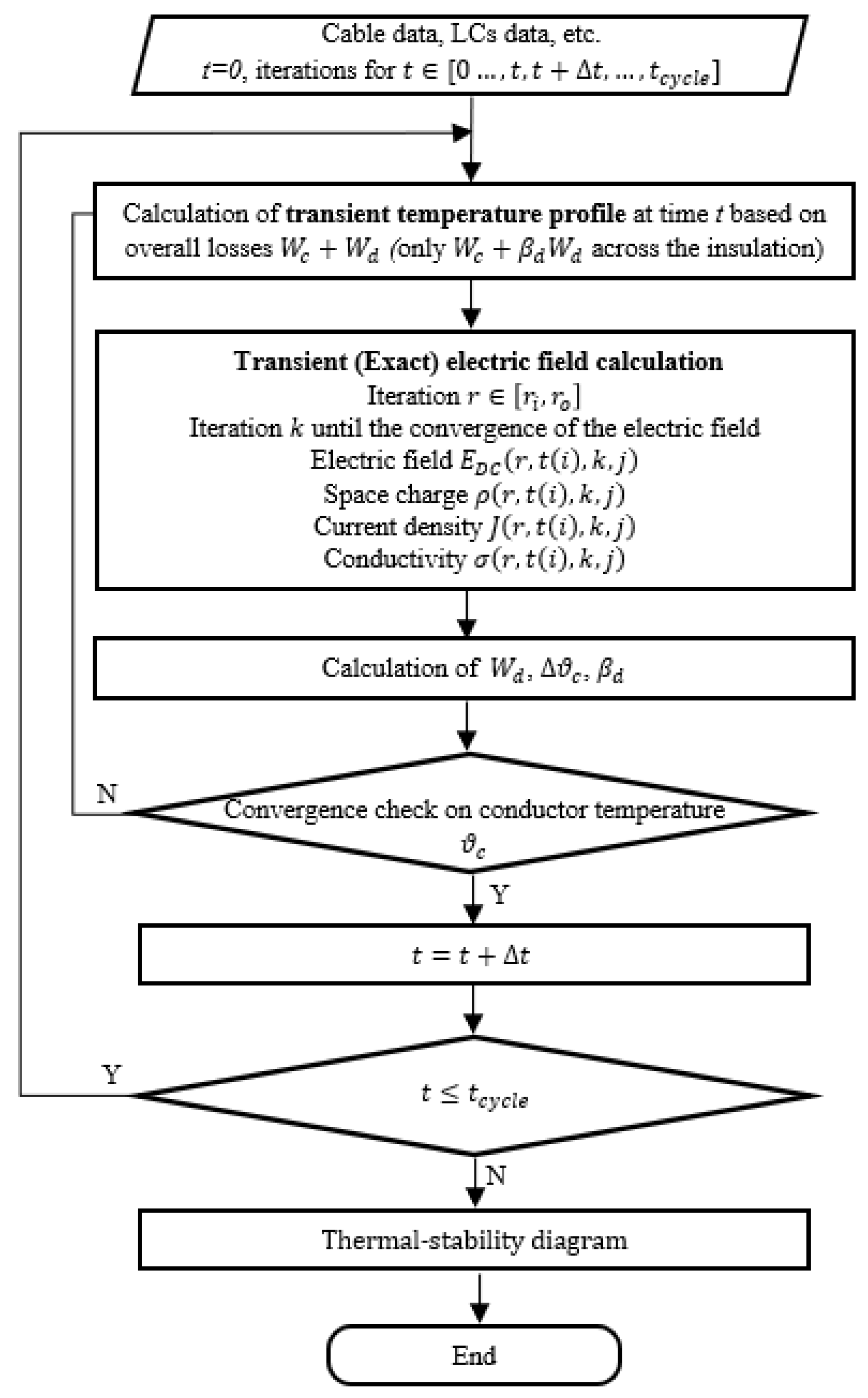
Figure 2.
The conductor’s and insulation’s current densities from (a) 3D perspective, (b) cross-sectional 2D perspective.
Figure 2.
The conductor’s and insulation’s current densities from (a) 3D perspective, (b) cross-sectional 2D perspective.
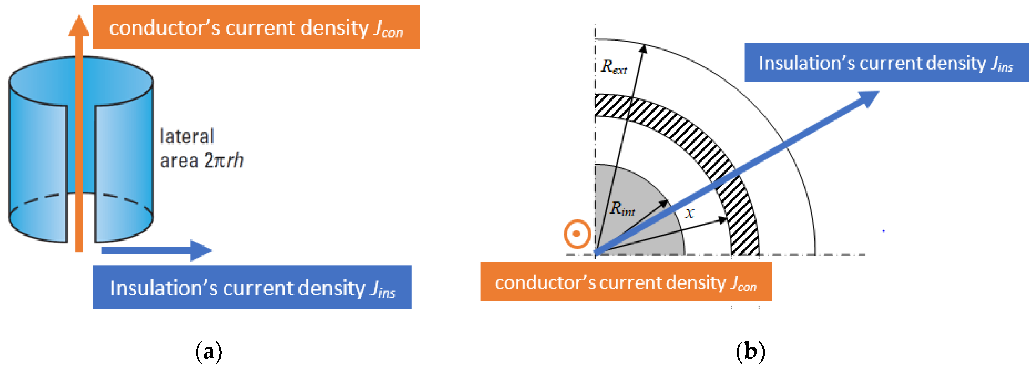
Figure 3.
The cross-sectional structure of the XLPE high voltage direct-current (HVDC) cables, with the temperature drops in the insulation, sheath and soil.
Figure 3.
The cross-sectional structure of the XLPE high voltage direct-current (HVDC) cables, with the temperature drops in the insulation, sheath and soil.
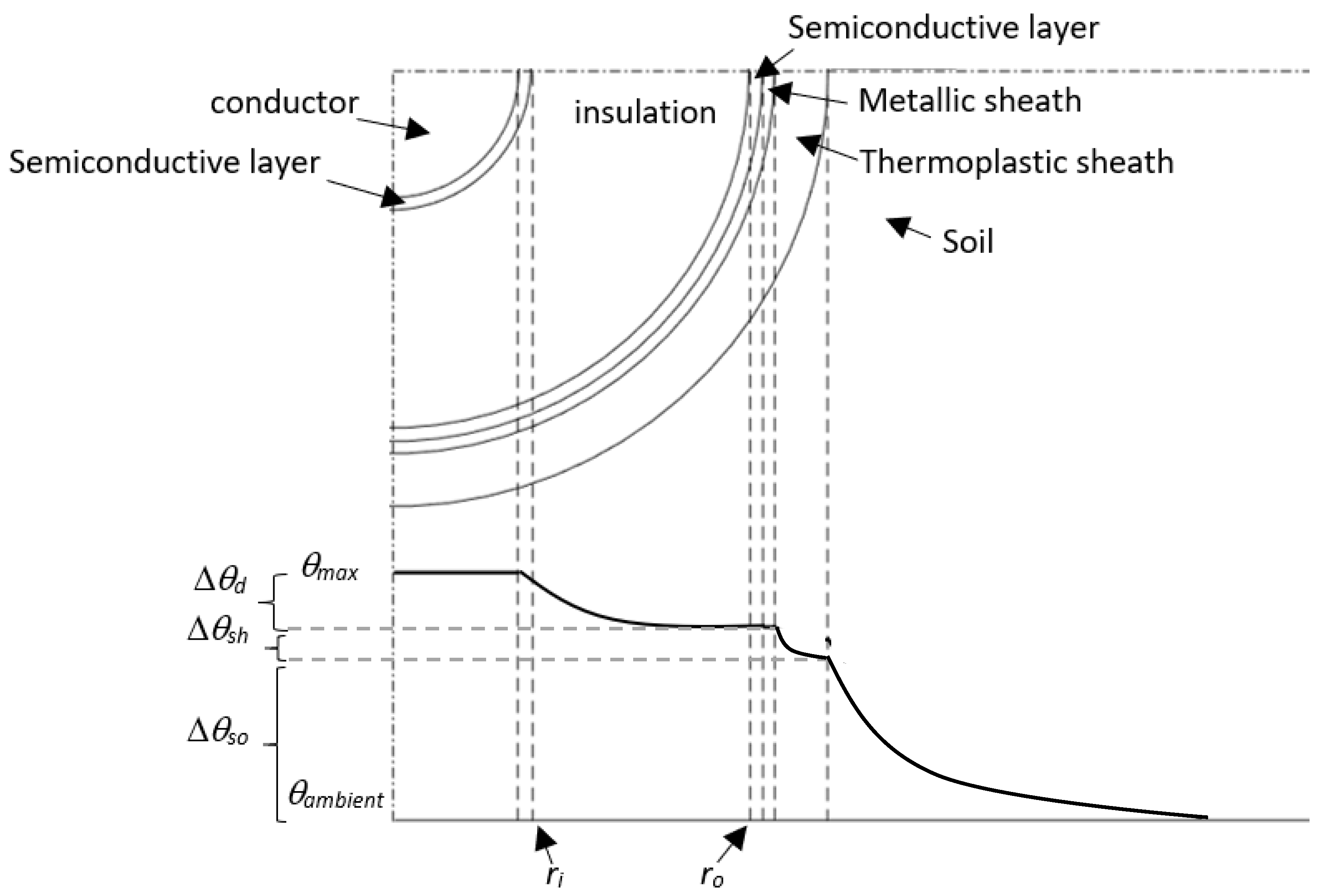
Figure 4.
The thermal stability diagram.
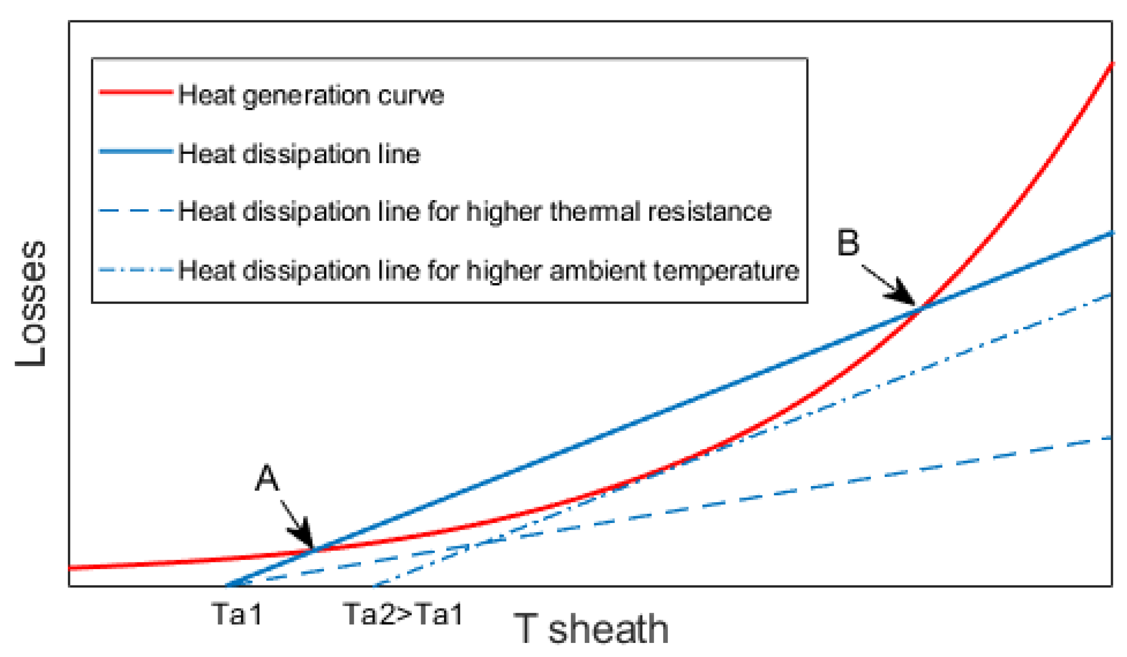
Figure 5.
The temperature profile of (a) 320 kV cable, (b) 500 kV cable at five points inside the insulation in the case of applying a 24-h load cycle according to CIGRÉ Technical Brochure 496 [6].
Figure 5.
The temperature profile of (a) 320 kV cable, (b) 500 kV cable at five points inside the insulation in the case of applying a 24-h load cycle according to CIGRÉ Technical Brochure 496 [6].
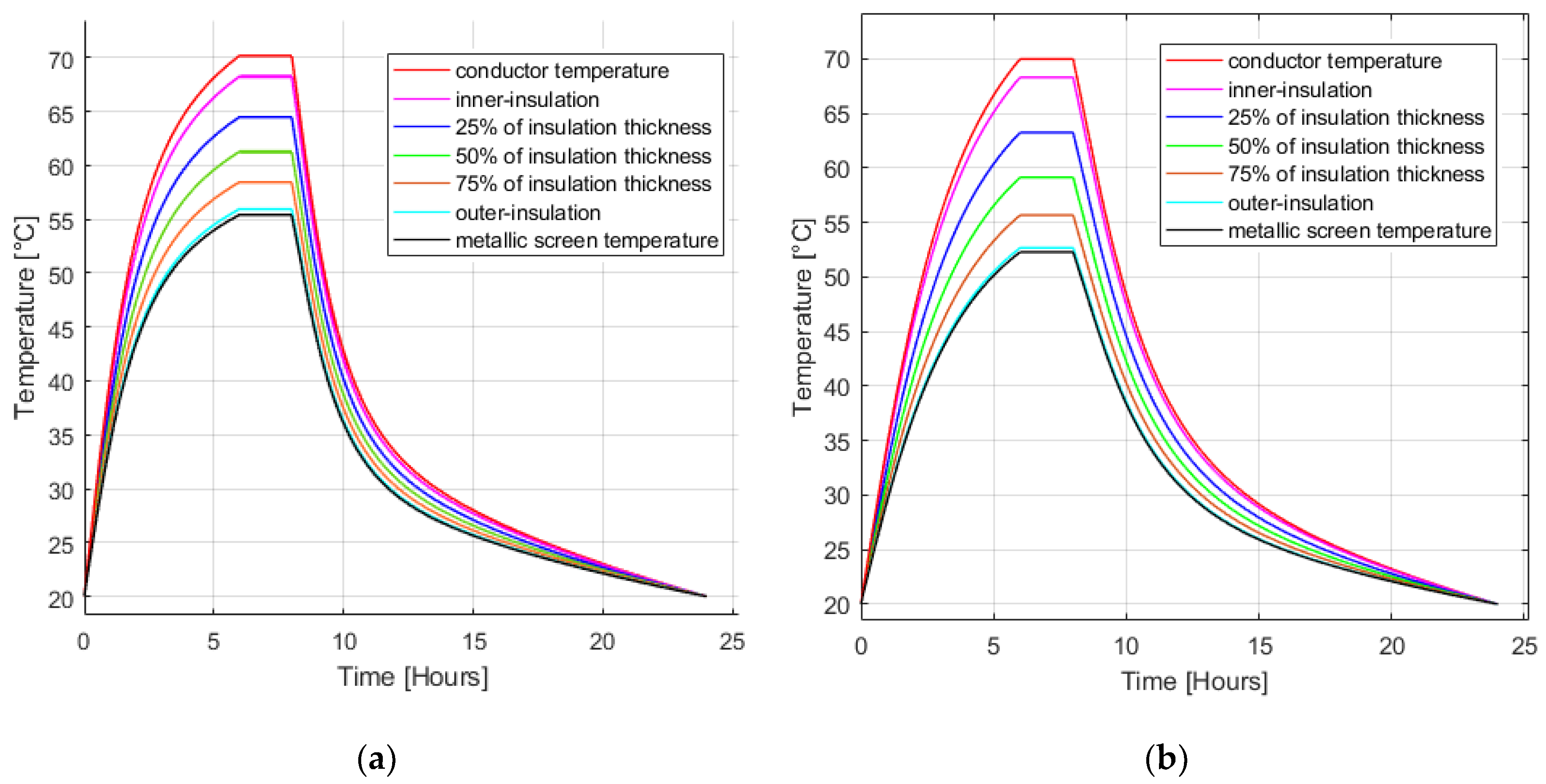
Figure 6.
The electric field distribution in the insulation of (a) 320 kV cable, (b) 500 kV cable, during the first 24-h load cycle of the load cycle period according to CIGRÉ Technical Brochure 496 [6].
Figure 6.
The electric field distribution in the insulation of (a) 320 kV cable, (b) 500 kV cable, during the first 24-h load cycle of the load cycle period according to CIGRÉ Technical Brochure 496 [6].
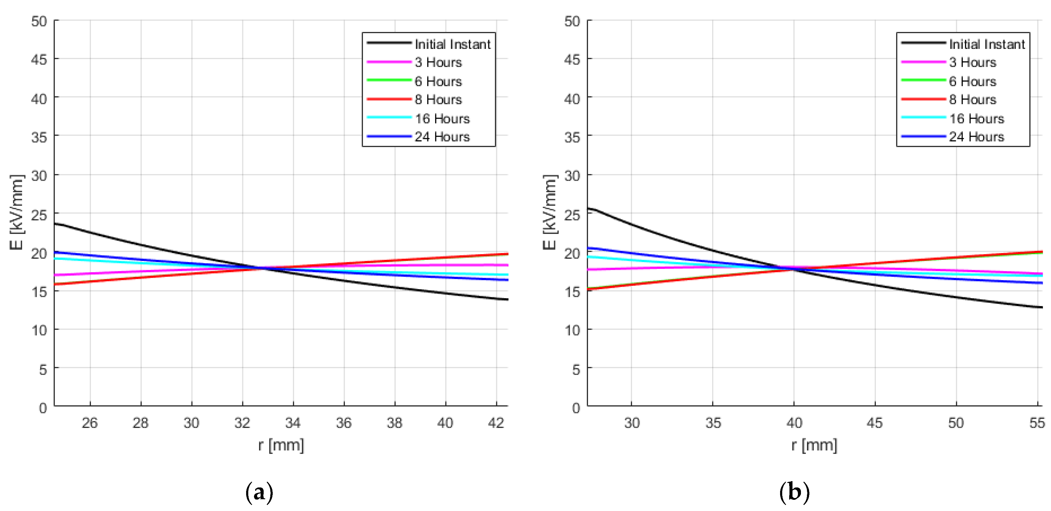
Figure 7.
The DC electric field profiles in the insulation of the 320 kV cable for different applied voltages: (a) at the ambient temperature (cold cable), (b) in the high load period according to CIGRÉ Technical Brochure 496 [6] (hot cable).
Figure 7.
The DC electric field profiles in the insulation of the 320 kV cable for different applied voltages: (a) at the ambient temperature (cold cable), (b) in the high load period according to CIGRÉ Technical Brochure 496 [6] (hot cable).
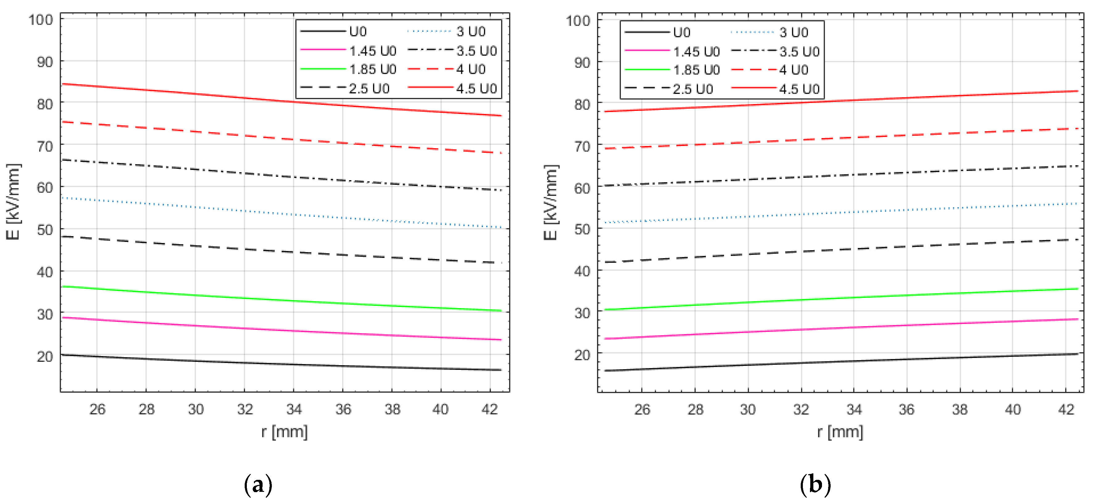
Figure 8.
The electrical conductivity profiles in y-log scale inside the insulation of the 320 kV cable for the different applied voltages: (a) at the ambient temperature (cold cable), (b) in the high load period according to CIGRÉ Technical Brochure 496 [6] (hot cable).
Figure 8.
The electrical conductivity profiles in y-log scale inside the insulation of the 320 kV cable for the different applied voltages: (a) at the ambient temperature (cold cable), (b) in the high load period according to CIGRÉ Technical Brochure 496 [6] (hot cable).

Figure 9.
The leakage current of the 320 kV cable in y-log scale for different applied voltages during the first 24-h load cycle of the load cycle period according to CIGRÉ Technical Brochure 496 [6].
Figure 9.
The leakage current of the 320 kV cable in y-log scale for different applied voltages during the first 24-h load cycle of the load cycle period according to CIGRÉ Technical Brochure 496 [6].
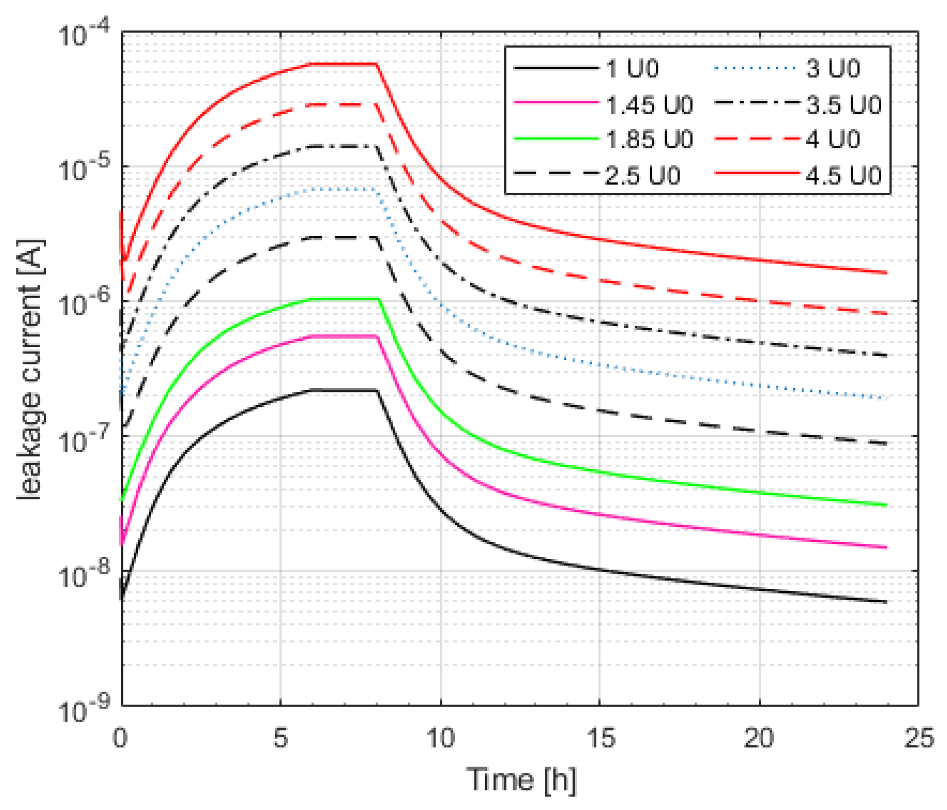
Figure 10.
The insulation losses of (a,b) the 320 kV cable and (c,d) the 500 kV cable in both linear (a,c) and logarithmic (b,d) y-scale during the first 24-h load cycle of the load cycle period after [6].
Figure 10.
The insulation losses of (a,b) the 320 kV cable and (c,d) the 500 kV cable in both linear (a,c) and logarithmic (b,d) y-scale during the first 24-h load cycle of the load cycle period after [6].
Figure 11.
The temperature rise of the hot vable due to insulation losses added to conductor losses vs. the position within the insulation thickness for increasing values of applied voltages with 3 sets of conductivity coefficients: (a) aL, bL; (b) aM, bM; (c) aH, bH. 320 kV cable.
Figure 11.
The temperature rise of the hot vable due to insulation losses added to conductor losses vs. the position within the insulation thickness for increasing values of applied voltages with 3 sets of conductivity coefficients: (a) aL, bL; (b) aM, bM; (c) aH, bH. 320 kV cable.
Figure 12.
The temperature rise of the hot cable due to insulation losses added to conductor losses vs. the position within the insulation thickness for increasing values of applied voltages up to 4.5 times the rated voltage with the medium set of conductivity coefficients aM, bM. 500 kV cable.
Figure 12.
The temperature rise of the hot cable due to insulation losses added to conductor losses vs. the position within the insulation thickness for increasing values of applied voltages up to 4.5 times the rated voltage with the medium set of conductivity coefficients aM, bM. 500 kV cable.

Figure 13.
Dielectric loss coefficient during the first 24-h load cycle of the load cycle period after [6]. 320 kV cable.
Figure 13.
Dielectric loss coefficient during the first 24-h load cycle of the load cycle period after [6]. 320 kV cable.

Figure 14.
The thermal stability diagram for (a) the 320 kV cable and (b) the 500 kV cable for different applied voltages up to 4.5 times the rated voltage.
Figure 14.
The thermal stability diagram for (a) the 320 kV cable and (b) the 500 kV cable for different applied voltages up to 4.5 times the rated voltage.
Figure 15.
The insulation losses vs. the mean electric field in the insulation for different values of temperature and stress coefficients of electrical conductivity a, b as reported in Table 4 at the maximum conductor losses (full load).
Figure 15.
The insulation losses vs. the mean electric field in the insulation for different values of temperature and stress coefficients of electrical conductivity a, b as reported in Table 4 at the maximum conductor losses (full load).
Figure 16.
(a) The de-rated conductor current w.r.t times the rated voltage, (b) de-rating factor w.r.t times the rated voltage for both the 320 kV and 500 kV cables.
Figure 16.
(a) The de-rated conductor current w.r.t times the rated voltage, (b) de-rating factor w.r.t times the rated voltage for both the 320 kV and 500 kV cables.


Table 1.
Cable characteristics.
| Parameter | 500 kV Cable | 320 kV Cable |
|---|---|---|
| Rated power (bipolar scheme) (MW) | 1715 | 1105 |
| Rated voltage (kV) | 500 | 320 |
| Conductor Material | Cu | Cu |
| Insulation Material | DC-XLPE | DC-XLPE |
| relative permittivity | 2.3 | 2.3 |
| Rated conductor temperature (°C) | 70 | 70 |
| Ambient temperature a (°C) | 20 | 20 |
| Conductor cross-section (mm2) | 2000 | 1600 |
| inner insulation radius ri (mm) | 27.2 | 24.6 |
| Insulation thickness (mm) | 28.1 | 17.9 |
| outer insulation radius ro (mm) | 55.3 | 42.5 |
| Design life LD (years) | 40 | 40 |
| Design failure probability PD (%) | 1 | 1 |
| Rated or design current (ampacity) Ic,n (A) | 1715 | 1727 |
Table 2.
Thermal characteristics of cable and environment.
| Thermal Resistivity | Thermal Resistance | ||
|---|---|---|---|
| 500 kV | 320 kV | ||
| insulation | 3.5 | 0.447 | 0.365 |
| Thermoplastic sheath | 3.5 | 0.0421 | 0.054 |
| Soil | 1.3 | 0.769 | 0.818 |
Table 3.
The conductivity coefficients of HVDC cable insulation for different types of dielectrics.
| Type of Dielectric | a (1/°C) | b (mm/kV) |
|---|---|---|
| Paper | 0.074 | 0.018 ÷ 0.029 |
| Thermoset | 0.084 ÷ 0.101 | 0.0645 |
| Thermoplastic | 0.104 ÷ 0.115 | 0.034 ÷ 0.128 |
Table 4.
Cable characteristics.
| Classification | Symbols of the a, b Set | M (Multiplier of aM, bM) | a (1/°C) | b (mm/kV) |
|---|---|---|---|---|
| Low set | aL, bL | 0.5 | 0.042 | 0.032 |
| 0.6 | 0.05 | 0.0387 | ||
| 0.7 | 0.059 | 0.045 | ||
| 0.8 | 0.067 | 0.052 | ||
| 0.9 | 0.076 | 0.058 | ||
| Medium set | aM, bM | 1 | 0.084 | 0.0645 |
| 1.1 | 0.092 | 0.071 | ||
| High set | aH, bH | 1.2 | 0.101 | 0.0774 |
| 1.3 | 0.109 | 0.0839 | ||
| 1.4 | 0.118 | 0.0903 | ||
| 1.5 | 0.126 | 0.0968 | ||
| 1.6 | 0.134 | 0.1032 | ||
| 1.7 | 0.143 | 0.1097 | ||
| 1.8 | 0.1512 | 0.116 | ||
| 1.9 | 0.156 | 0.1225 | ||
| Very high set | aVH, bVH | 2 | 0.168 | 0.129 |
Publisher’s Note: MDPI stays neutral with regard to jurisdictional claims in published maps and institutional affiliations. |
© 2021 by the authors. Licensee MDPI, Basel, Switzerland. This article is an open access article distributed under the terms and conditions of the Creative Commons Attribution (CC BY) license (http://creativecommons.org/licenses/by/4.0/).
Share and Cite
MDPI and ACS Style
Diban, B.; Mazzanti, G. The Effect of Insulation Characteristics on Thermal Instability in HVDC Extruded Cables. Energies 2021, 14, 550. https://doi.org/10.3390/en14030550
AMA Style
Diban B, Mazzanti G. The Effect of Insulation Characteristics on Thermal Instability in HVDC Extruded Cables. Energies. 2021; 14(3):550. https://doi.org/10.3390/en14030550
Chicago/Turabian StyleDiban, Bassel, and Giovanni Mazzanti. 2021. "The Effect of Insulation Characteristics on Thermal Instability in HVDC Extruded Cables" Energies 14, no. 3: 550. https://doi.org/10.3390/en14030550
Note that from the first issue of 2016, this journal uses article numbers instead of page numbers. See further details here.