Abstract
We explore some rheological aspects of the yielding of gelled waxy crude oil on the basis of a fractal model for the structural description of the waxy gel and Marrucci’s model for the time evolution of the stress with mixed elastic and viscous effects. With some parameters of the model directly obtained from classic rheometry, and others by fitting the parameters to the experimental data of one shear-rate condition, the flow curves for another shear-rate condition are predicted. Both theoretical curves—the fitting and the predicted ones—share the basic features of the experimental ones. Comparison with results of Maxwell model shows that Marrucci’s model used here leads to much better results, as it incorporates nonlinear viscoelasticity of waxy crude gels in the stress evolution equation. The strain dependence of the elastic modulus also plays a relevant role on the prediction of the model, suggesting a double-network contribution for very small strain values. Due to the inertia of rheometric device, the actual shear rate is often found to depart from the setting one, and modification of shear rate history can be necessary in model validation.
1. Introduction
The rheological behaviors of gelled waxy crude oils during yielding process is a very relevant problem for theoretical rheology, as it exhibits the consequences of drastic structural modifications at a microscopic level, leading the system from a solid-like behavior to a thixotropic fluid behavior. Furthermore, it is also very useful because it may help engineers make smart decisions on the operation strategies for pipelines. For instance, before it enters the pipeline, waxy crude oil is often heated to a relatively high temperature to keep it from gelation. While during pipeline shutdown, heat supplement no longer enters the pipe and drastic temperature drop could happen. As a result, waxy components once dissolved in waxy crude may precipitate from the oil when the temperature falls below its wax appearance temperature (WAT). If the shutdown lasts for a long time, irreversible gelation could happen in the pipe since a more stable structure has developed due to high fraction of wax precipitates. Quantitative description of the viscoelastic behavior of a waxy crude gel is helpful in estimating the minimum pressure and time needed to restart the flow after a period of shutdown [1,2,3,4]. Such practical relevance and consequent economic implications of yielding behavior add to its theoretical interest and experimental challenges, making it a topic of great significance. In this work, we aim to model this nonlinear viscoelastic behavior of waxy crude oil as the yielding of a fractal gel.
The yielding behavior of waxy crude oil has many complexities [5,6,7,8,9,10,11]. The flow curves in Figure 1 (whose experimental details will be fully discussed in Section 3) are typical ones of yielding. To quantitatively describe them, two forms of thixotropy models have been developed, both of which consist of an evolution equation for stress and for the structure, characterized by an abstract structure parameter , varying from 1 (pure elastic behavior) to 0 (pure viscous behavior). Depending on the rheology of the stress equation, the two categories are often named as the viscoplastic thixotropic models and the viscoelastic thixotropic models.
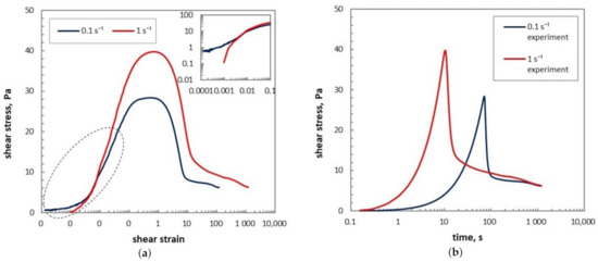
Figure 1.
Experimental results of the evolution of shear stress during yielding of an initially gelled waxy crude oil: (a) as a function of shear strain; (b) as a function of time t. Data provided by Zhang [12].
The viscoplastic thixotropic models widely adopted in the oil industry are developed on the basis of a pseudo-plastic model, such as the Bingham model or the Herschel-Buckley model [13,14,15,16]. These models consider the waxy gel as a rigid body before yielding and as a viscous fluid with decreasing viscosity with time immediately after a critical stress is loaded. The viscoelastic models, or the elasto-viscoplastic models, incorporate the description of viscoelasticity during pre-yielding period by using stress equation [17,18,19,20]. In most of these models, the yield stress term of a steady viscoplastic model is simply replaced with elastic stress. Since the structure-dependent yield stress well reflects the qualitative features of thixotropy during yielding, the predictive ability of these two kinds of models is usually found to be quite satisfactory [21].
The shortcoming of the viscoplastic thixotropic models is obvious. They fail to give a rheological description in the pre-yielding region. Moreover, the presence of the yield stress even after yielding in those models is theoretically problematic. Further problems of the existing viscoelastic-thixotropic models for crude oils are: (1) Their stress equations are not developed on mechanical basis, and the steady-state shear stress-shear rate relationship could not be recovered by setting the time derivatives in the evolution equation to zero; (2) Too many parameters with no specific physical meaning have to be determined through complex numerical fitting.
Alternatively, the models based on a linear viscoelastic stress equation developed from classic mechanical models, such as Maxwell model or Jeffrey model, are able to describe the pre-yielding rheological behavior, and thus enhance their theoretical interest [22,23,24,25,26,27], among which the model proposed by de Souza Mendes and R. L. Thompson [27] has been modified and applied to describe the rheological behavior of waxy crude oil by Van Der Geest et al. [28]. However, quantitative description of the gel microstructure evolution in the early stage of yielding does not contribute to any of these models, since most them are not developed on the basis of actual material, so that experimental aspects could not be taken advantage of in understanding the yielding mechanics. As a result, all of them use an ambiguous structure parameter to describe the structure, which seems very difficult to validate. Moreover, using a linear viscoelastic stress model (such as Maxwell or Kelvin-Voigt model), the effects of the thixotropy caused by drastic structural changes during yielding process on the mechanical properties, i.e., the dependence of the elastic modulus G and the viscosity on time t, is not accounted for. However, since thixotropy is caused by structural evolution of the gel, it should have been taken into consideration as a main character when modeling the yielding of structured gels such as waxy crude oil itself. Mendes et al. [29] have chosen a different way of modelling the rheological behavior of waxy crude oil by involving both flow and temperature history dependence, based on new findings about the structure destruction characteristics from the experimental results of waxy crude oil. Since waxy crude oils are complicated mixtures with special characteristics, their rheological modelling needs further studies.
In this paper, for the evolution equation of shear stress, we employ a nonlinear viscoelastic model proposed by Marrucci and used to model the viscoelasticity of structured polymers [30,31,32,33,34]. We propose an explicit identification for the structure parameter , which is often used in an abstract way in other thixotropic models [16,17,18,19,22,23,24,25,26,27], and incorporate the structure change by relating to the several material coefficients in the stress equation. In order to do so, we consider the gel as a fractal structure with a characteristic fractal dimension D. Based on a model for the yielding of weakly flocculated suspensions [35,36], we are able to estimate the viscosity and the discussion of the yielding point from a microscopic point of view, in terms of a characteristic radius . Another particular aspect we consider here is the time variation of shear rate (and therefore of shear strain ). Instead of assuming as an imposed constant along the whole process, we find the inertial transient behavior from 0 s to the final imposed steady-state value of with an overshoot in between. We use expressions closer to the experimental observations and analyze their influence on the results. This noteworthy influence occurs in the yielding experiments when the imposed shear rate is driven by a controlled-stress rheometer, which is not rare in References [7,8,20,29,37], considering the fact that controlled-stress rheometers are more common than controlled-strain ones.
The article is organized as follows—in Section 2, we discuss the evolution of the structure during yielding from the microscopic perspective, based on which the theoretical justification of the model and its viscoelastic description for both elastic modulus G and viscosity is proposed. In Section 3, experimental protocols and material properties used to obtain the rheological parameters of the model so as to validate the model are presented. In Section 4 and Section 5, we summarize detailed computing method of the model, and then present the results under different hypotheses and comment on the merit and weakness of each one. In Section 6, the concluding remarks are given and the direction of future investigation is discussed.
2. Theory
Our aim is to express the shear stress as a function of strain or of time t in the yielding region. First, we use a fractal model proposed by Snabre and Mills [35,36] to interpret the structural evolution of the waxy crude gel corresponding to its mechanical behavior in yielding, and to analyze the critical strain of yielding, which will be used in the following modelization. For the macroscopic description of the evolution of containing both elastic and viscous contributions, we use a thixotropy modelization similar to that in earlier works [23,25,32,38].
2.1. Microscopic Description
In this section, we use a blob model to characterize the flocculated clusters in the waxy crude gel. Under this assumption the critical transition conditions between two successive stages and microstructural changes during each stage will be analysed, among which the most important transition condition—the critical strain of fracture yielding—will be estimated theoretically.
2.1.1. Fractal Model of the Gel
Pioneer studies in References [8,39,40] show that rheological properties, for instance, the viscosity and elastic modulus of waxy crude oil, may be well described by fractal models. Also, waxy crude gels and fractal systems have been found to have many morphological features as well as gelation mechanisms in common [9]. Therefore, from experimental point of view, waxy crude oil shares many basic features with fractal models. Here, we consider waxy crude gel as a fractal cluster network constituted by gel clusters of characteristic size accumulating primary spherical particles of smaller size a (precipitated wax crystals, in our case), and characterized by fractal dimension D, meaning that the number N of primary particles in each cluster depends on a, and as
Furthermore, following Snabre and Mill’s work [35,36], we assume that the clusters in waxy crude oil may be conceptually considered as spherical blobs of radius , filling the volume of the system with a volume fraction of and a maximum packing volume fraction of ( for random packing of rigid spheres). The sketch of the configuration of the blobs in different stage of yielding in Figure 2 is to help understand the yielding of the gel from the microscopic prospective. As long as it is in the gel state, the blob radius is assumed to stay , and the volume fraction occupied by the blobs will always be . After the blobs are broken and the system enters the sol state, will decrease with following the time evolution equation which may be obtained from the kinetic equation of the structure parameter (see Section 2.2.2). Because of the fractal assumption Equation (1), both and may be related to the volume fraction of the primary particles as [8]
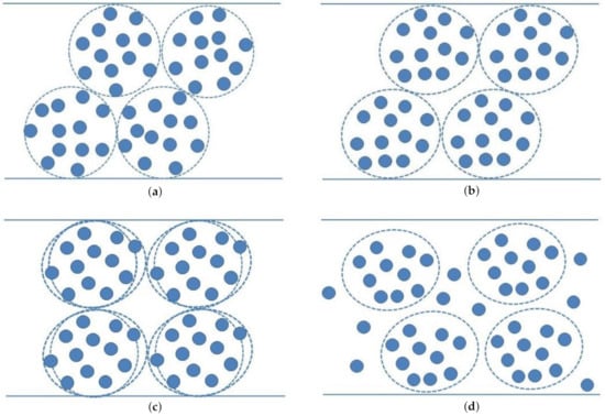
Figure 2.
Blob model illustrating the microstructure evolution during yielding: (a) intact gelation structure; (b) microstructure during elastic dominant viscoelastic creeping; (c) microstructure with tangency geometry at critical point of structural yielding; (d) breaking of colloidal aggregates after the structural fracture of gel.
Thus, the relationship between and , both before and after the breaking of the blobs, could be described by
2.1.2. Microstructure Evolution and Characteristic Transition Points
As from the macroscopic point of view, the mechanisms during different stages of yielding—elastic deformation region, creeping stage, and fracture stage—are significantly different, we put our focus on interpreting what happens to the microstructure in each stage, and discuss the rheological behavior separately as well. From the flow curves in Figure 1a, four distinct regions can be identified:
- The initial overlapping part of the two curves (corresponding to different nominal values of the shear rate )—from the beginning up to point A—can be interpreted as an elastic deformation of the gel, with an infinite or extremely high viscosity;
- The region between point A and peak-stress point B can be interpreted as to a viscoelastic creep, where elastic modulus decreases and viscosity becomes finite, but elastic behavior still dominates;
- In the region beyond the peak point B up to the inflexion point C, viscous flow becomes increasingly dominant and the microstructure of the initial gel breaks in a steep way, leading to a reduction in both elastic modulus and viscosity;
- The region between point C and the steady-state point D corresponds to thixotropic behavior of the the remaining structure, mostly a viscous behavior with the viscosity decrease slowing down until a steady-state is achieved.
Upon the blob assumption of the microstructure of the gel proposed in Section 2.1.1, we may interpret the critical points on the flow curves in Figure 1a as follows: (1) point A as the elastic-limit point where bonds between gel particles inside the blobs begin to break (when the spherical blobs are increasingly turned into ellipsoidal blobs); (2) point B as the structure fractural yielding point (corresponding to the strain value ) where the blobs become able to move relatively to each other because of the removing of the geometric constrictions to their motion so that the gel network collapses as a whole and the blobs begin to break; (3) point C (corresponding to the strain value ) as the inflexion point, where breaking process begins to slow down.
From the beginning up to point A, the gel deforms elastically and one may imagine this as a relative deformation of the blobs with the density of bonds between them staying constant (Figure 2a). From point A to Point B, further deformation breaks internal bonds and stretches out the blobs from spheres into ellipsoids in the direction of shear. The breaking of the bonds will lead to a reduction of the elastic effects, while the orientation of the blobs will make more space for them to move, thus generating viscous effect. But as long as , the bond density still stays high enough to hold all those primary particles inside the blobs where they originally belong to (Figure 2b). And since the volume fraction of the blobs does not change, it will remain in the gel phase. For , that is, from point B to C, the bonds break with an increasingly reduced proportion and there are small particles leaving their original blob. Thus, the blobs become small enough to freely move with respect to each other, and the system enters the sol phase (Figure 2c). For that is, from point C to D, the bonds between particles in individual blobs become weaker due to larger strain and more intense shear, and thus the radius of the blobs will decrease with time (Figure 2d).
2.1.3. Estimation of the Yield Strain
While the thixotropy models of waxy crude oil have always given a satisfactory description of the fourth stage (from C to D), our focus will, alternatively, be the first three stages, that is, from the beginning to C, which are closely related to the transition from gel to sol state.
To estimate the value of , let us consider four of the spherical blobs in contact in the compact gel, each one of radius , two in the upper line and the other two in the lower line (see Figure 3a). The separation l between the upper and lower horizontal planes in tangent contact with the spheres is . In the configuration of the Figure 3a, the upper sphere cannot move with respect to the lower ones, because of geometric restrictions. In Figure 3b, two deformed ellipsoidal blobs may stand vertically one over the other, and thus relative motion is enabled. In such critical configuration, the critical radius of the inscribed circle of any blob ellipse, whose semi-minor axis is equal to , may be given by .

Figure 3.
Sketch for an estimation of the yielding shear strain: (a) before elongation; (b) at critical elongation.
A direct estimation of critical strain is given by the tangent of the angle formed by the lines AC and BC in Figure 3a. In order that the upper sphere may slide over the lower one (with some vertical contraction of both of them), the contact point A of both spheres must arrive at position B. The corresponding tangent is given by , which provides an alternative estimation for the critical strain. In fact, the actual yield point is expected be somewhat smaller than 0.27 if one takes into account that the spheres will be compressed in the vertical direction as they are sheared one with respect to the other.
Alternatively, we may estimate the yield strain in a more accurate way. The deformation is a combined effect of shear and contraction. We assume a horizontal displacement along the upper surface due to simple shear, plus a vertical contraction. In order to start relative motion, the blob must be tilted with an angle , whose cosine may be expressed as , with half the distance between the two points (B’ and C’ in Figure 3b) on the elliptical blob in contact with neighboring blobs, and equal to its critical vertical projection. The vertical projection (as obtained in the former paragraph), and may be taken as an approximation, in such a way that , and . Actually, the distance between B’ and C’ is slightly lower than , so the actual yield strain must be lower than 0.40. We may estimate this strain more precisely with the aid of analytic geometry, and the results is shown to be 0.25 (see Appendix A).
In our analysis we will take (see Table 3). The experimental results of yield strain 0.2 at 31 C to 1.0 at 35 C [41] are indeed in this range.
2.2. The Model
In this section, the theoretical concept of the development of the model will be given in detail. Based on a viscoelastic model for the description of mechanics, a kinetic equation for the structure and two material functions for the rheological parameters of the gel at a certain structured level are also proposed.In the viscoelastic model, two material parameters appear—the elastic modulus G and viscosity , which depend on the structure of the material, and on and . To close the description, an evolution equation of the structure and its relation to G and are needed. Thus, two evolution equations, for the stress and for the structure parameter are needed, complemented with functions for , appearing in the stress equation, and for the building-up and the destruction terms of structure and , appearing in the evolution equation for , respectively. For the sake of higher efficiency, we will slightly modify the general scheme of modeling the kinetics for the structure by expressing it in terms of .
2.2.1. Mechanical Description: The Nonlinear Viscoelastic Model
In previous models, the evolution of shear stress is often described by linear viscoelastic models like Maxwell-like or Jeffrey-like models, which do not account for the time-dependent behavior of G. In our model, instead, the shear stress will be described by the nonlinear viscoelastic model
Equation (4) could be seen as the nonlinear version of Maxwell model. It has the same mechanical analogical model as Maxwell model, only with the time dependence, or the strain dependence of the material parameters considered. And it reduces to the Maxwell model upon constant and G. This kind of model was first used by Marrucci et al. [30,31,32,33,34] for the description of structured suspensions viscoelasticity, but so far has not been applied to waxy crude oil, whose elastic modulus G dependence on time t or on shear strain should not be ignored as well due to the dramatic structural changes during its yielding. The shear modulus and the viscosity will be given in Section 2.2.3 as Equations (14) and (15) respectively. We will show that Equation (4) leads to better results than using the linear Maxwell equation in the discussion Section 5.2.
2.2.2. Kinetic Equation and Physical Interpretation of the Structure Parameter
The second aspect to be considered is the structure evolution of the system, which in its turn influences G and . Since the microstructure is very complicated, it is usually simplified as a scalar parameter which goes from for the completely structured gel to for the completely unstructured fluid [16,17,18,19,22,23,24,25,26]. Of course, this is a very radical simplification, but it may cause ambiguity in modelling and validation. So in this section, we will first make our definition for the structure parameter on the basis of the features of the microstructure of the gel.
a. Physical interpretation of
In searching for an explicit physical interpretation for the structure parameter , let us recall the microstructure of the gel, which has been discussed in Section 2.1.1. Since is the main feature that describes the gel structure, we define our structure parameter as
In the system of a fractal gel, while the microstructure is often characterized by size , the material parameters such as the elastic modulus and viscosity are mostly affected by the the concentration of gel clusters. Therefore, an expression for in terms of the volume fraction of the mentioned blobs , rather than in terms of their radii is needed. According to the relation between and described by Equation (3), the structure parameter may also be interpreted as
Note that for the fully gel phase, and ; and to the completely unstructured fluid , and , as usually required to recover the steady-state viscosity relation. Note, finally, that a yet more detailed analysis could assume a lamellar structure of the gel instead of an isotropic fractal structure, as observed in microscopic analyses [42], but we will leave these details for future work. Furthermore, the fractal dimension D itself could change along the yielding process, but here we kept it constant.
b. Kinetic equation for
The evolution of the structure parameter consists of a build-up term describing structure formation and a destruction term describing structural degradation. Both terms depend on the shear conditions, and thus may be expressed in terms of stress [25,26,27], of the shear strain [37], or of the dissipation rate [18,23]. In the literature, this equation is often expressed as
with , the times characterizing the growth and decay of , and , characteristic exponents. describes the structural evolution dependence on the instantaneous shear condition, which could be assumed, for instance, to be a univariate dependence on as References [17,19,37] did in their work.
Departing from the assumption that is decreasing from the very beginning of loading () made in other models [25,26,27], we assume that as long as the gel structure maintains intact, and only begins to decrease after the critical strain for yielding (which has been discussed in Section 2.1.2). Thus, in Equation (7) could be
in which is the Heaviside step function with a zero value for and unit value for , is the shear rate above which most of the blobs have become primary particles, and n is an exponent. If we take for simplicity, we obtain the steady state value of
In the recent work of Mendes et al. [29], the microstructure evolution was found to depend more directly on shear strain, rather than on shear rate. Moreover, as is discussed in Section 2.1.2 , the yielding point may also be interpreted in terms of shear strain, therefore, instead of expressing the changing rate of structure in terms of t like Equation (7), here we choose to express the evolution of directly as a function of shear strain . They also proved that the extent of structure destruction depends on the most severe shear condition that the oil gel has experienced during its yielding process, which in our case would be the steady-state shear rate. Thus, we consider a same steady-state structure as given by Equation (9), and propose the evolution of structure parameter following relaxation equation of as
where is a value of the shear strain characterizing the change of from the initial value to the steady-state value of . Of course, the time-dependence rate of may be obtained as in Equation (10), by applying the chain rule . This is especially easy if the dependence of shear rate on time is explicitly given, for instance, if a constant, stepwise or oscillatory shear rate is applied on the system. However, in the particular situation under examination, where the shear rate depends on time in a more complicated way (see Section 4.1), it would take some serious effort to obtain the solution of Equation (7) as a function t, so we focus our attention on Equation (10) instead. Below, once is given, we may obtain . This is a further original aspect of the present work, which allows to consider the curve in a more direct way. Anyway, after considering , in Section 6, we will also be able to express the time evolution of the shear stress .
With the physical interpretation of in Equation (5), a shear-strain dependence of the evolution of , describing how the blob breaking in the region from point B to C in Figure 1a, may be obtained. Since the evolution equation of as a function of has been given by Equation (10), thus by solving it, one obtains the transition behavior of between and as
in which is the initial value of the blob radius corresponding to the radius of the maximum packing situation (gel state), and the steady-state radius. According to Equation (9), is also to depend on the imposed as
in which is phenomenological parameter related to the relaxation time of both blob break and particle reunion, is the critical strain above which most blobs have been breaking into primary particles, and q is an empirical exponent. This expression reflects the obvious fact that the characteristic blob radius will decrease with increasing , because primary particles will be stripped off more easily from the clusters. Thus, in the initial breaking region B ∼ C, decreases with , from its initial value to its steady-state value . Practically, all the parameters in Equation (12) could be obtained by fitting the steady-state viscosity at several , which are related to through relation Equation (15). Technically, these parameter could also be obtained through microscopic experiments. As for our analysis, it turns out , and fits the results well.
2.2.3. Material Functions and Rheological Properties
The other two functions needed to describe the process are G and appearing in Equation (4). The second one is dependent on , because viscosity of suspensions is known to strongly depend on the radius of particles. In contrast, no such strong dependence should be expected for G, because in the gel phase , and the only effect on G is that internal bonds between the blobs are increasingly broken with higher in the gel phase when the blobs deform.
a. Elastic modulus
We assume the elastic modulus G is proportional to the number density of full chains of bonds times the elastic constant of each bond, and a certain number of such bonds break at a given shear strain. According to this assumption, the nonlinear elastic modulus of the system is given by expression
with the equilibrium value of elastic modulus, the characteristic shear strain, and p the phenomenological exponent. Equation (13) of G exhibits a steep drop at after a plateau equal to for , and followed by a very small value for , with p controlling the steepness of the reduction of around . This form of is analogous to that used in References [16,43], with the difference that they used elastic part of shear strain instead of the directly measured strain . depends on the conditions of gelation, for instance, whether it was in a quiescent state or under shear, and how fast the cooling rate was [8]. It could be tested with rheometer by applying a small amplitude oscillatory shear to the waxy gel sample after it rests at the test temperature for a long time. Comparing the behavior of to that of our situation, and since a sudden reduction in G reasonably corresponds to the collapse of the gel network, will be taken close to the yield strain .
As the imposed shear rate is as low as 0.1 or 1 s, it is only reasonable to consider the initial behavior as purely elastic. Therefore, the elastic modulus G within the strain range could be calculated by . The calculated elastic modulus shown in Figure 4 is seen to start falling from a very high value at the very beginning of the deformation. This could arise from a pre-collapse of gel network at a rather small strain , which is hardly noticed because of its short-term existence. Thus, one may imagine, that besides the gel network which we have seen to break around the yield strain , with an equilibrium elastic modulus which can be obtained from rheometric test, there is another more brittle and rigid network in the gel, with smaller characteristic strain of breaking and higher initial elastic modulus . Such double network structure would have an elastic modulus equal to the summation of moduli of both networks, each of which is given in the form of Equation (13)
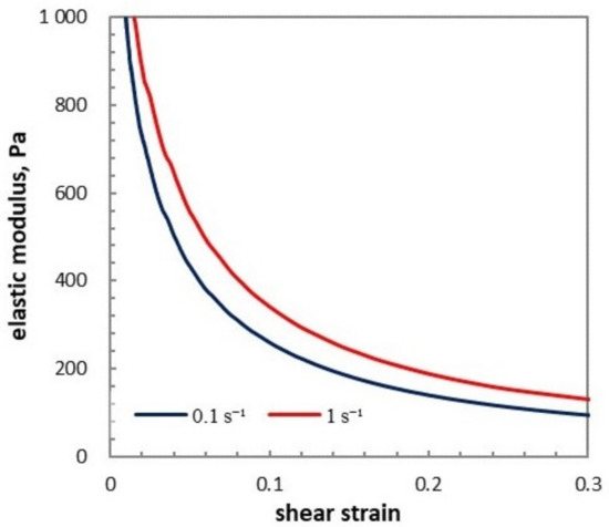
Figure 4.
Shear modulus dependence on shear strain in the early stage of yielding, obtained from the experimental data of and in Figure 1a by appling .
In practical terms, the critical shear strain would imply the strain for which the elastic modulus of the network i drops with a steepness characterized by (related to the fractal dimension of each network) due to the breaking of the corresponding type of bonds. Therefore, for small strains , one would have a plateau of modulus G of approximately , and between and , there might be another plateau of approximately , whose width and position depend on the separation between and and on steepness of the two drop behaviors, that is, on the values of exponents . This behavior may be caused by asphaltene or resin macromolecules which coexist with wax crystals. Its influence will be further explored and justified on experimental grounds in Section 5.1.
b. Viscosity
To estimate the viscous effect beyond point A, we use the viscosity model for suspensions with viscoelastic aggregates proposed by Snabre and Mills [35], which relates to the volume fraction of aggregates and deformation tensor as
where is the solvent viscosity, the maximum packing volume fraction (64% for random close packing of rigid spheres), is the component of the deformation tensor , and a parameter characterizing the viscous effect generated during creeping. For , we take a simple assumption that it is proportional to until the structural failure of the network, beyond which it becomes a saturated constant. Equation (15) is developed on the basis of a viscosity model for suspensions with rigidly flocculated blobs [35], by taking into account the effect of the elastic deformation of the blobs. Instead of being constant as in the model of the rigid-blob suspension, the effective maximum packing volume fraction in Equation (15) is assumed to increase with deformation as . This correction makes the volume fraction of the blobs smaller than so that a high but finite viscosity is expected before fracture yielding. It reflects the physics discussed in Section 2.1.1—since the blobs are elongated and become more orientated, bigger room is made for their movement. Thus, the internal flow through the network becomes less congested, leading to a higher fluidity, but still an inconspicuous viscous effect before the blobs are broken.
3. Materials and Experiments
Rheometric tests are taken to obtain the data we need to verify the model and differential scanning calorimetry (DSC) is used to detect the wax fraction precipitated from the oil varying with temperature. The material we use in the experiments is a typical waxy crude oil sampled from the Daqing oil field in the northeast of China, which is famous for its high wax content. In this section, a detailed description of the material as well as the procedure of the rheometry experiments will be given.
3.1. Materials
The wax appearance temperature (WAT) of the specimen we use is 44.8 C. It has a total wax mass fraction of 21.7%, with only 1.1% mass fraction precipitated by the test temperature 34 C. In Figure 5, the concentration profile of alkanes with different number of carbon atoms obtained by gas chromatography shows more detailed composition of the waxy crude sample. In order to eliminate the memory effect of flow and thermal history, all the samples were pretreated before the measurements. The samples sealed in 100-mL-gas-tight bottles were heated in a 80 C water bath for 2 h, statically cooled to room temperature, and maintained for 48 h before use.
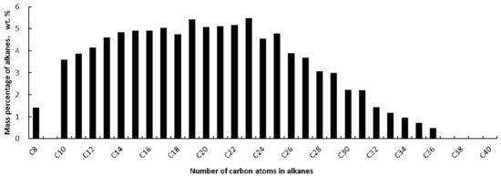
Figure 5.
Concentration profile of alkanes with different numbers of carbon atoms in the crude oil sample.
3.2. Differential Scanning Calorimetry
The Differential Scanning Calorimetry (DSC) test of the crude oil sample was conducted with a modulated DSC instrument (TA 2000/MDSC 2910,New Castle, DE, USA), and according to the regulation SY/T 0545-2012, China’s standard method for differential scanning calorimetry of the oil and gas industry. With the data of heat flow transmitted at each tested temperature (Figure 6a), the mass fraction of the precipitated wax as a function of temperature was obtained (Figure 6b). Figure 6a shows that the WAT (wax appearance temperature) of the waxy oil, corresponding to the point where heat flow slope turns non-zero, is 44.8 C. Figure 6b shows the sample has a total mass fraction of wax , but only 1.1% mass fraction has precipitated by the test temperature C.
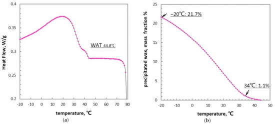
Figure 6.
Differential Scanning Calorimetry (DSC) curves of the waxy crude oil obtained in laboratory: (a) heat flow varying with temperature T. (b) mass fraction of precipitated wax varying with temperature T.
3.3. Small Amplitude Oscillatory Shear (SAOS)
A controlled-stress rheometer (HAAKE MARS III, Karlsruhe, Germany) equipped with a sensor system Z38 Ti of geometry of concentric cylinder was used to test the viscosity and shear modulus. The pretreated specimen sealed in blue cap bottles were heated from ambient temperature to 50 C (higher than WAT) in the water bath and were kept for 30 min. Then it was loaded into the concentric cylinder gap preheated to 50 C. The oil samples were cooled at a rate of 0.5 C/min from 80 C to 30 C, loaded with a small amplitude oscillatory shear, of a frequency of 1 Hz and a dynamic shear strain of 0.0002, which is small enough to preserve the structure. Meanwhile, the storage and loss moduli as well as the complex viscosity were tested and recorded. The data are presented in Figure 7. According to Figure 7, the gelation point of the waxy crude oil is 36 C, and the order of dynamic moduli at this point are as small as 1 Pa, meaning that a fully developed gel structure has not been achieved and yielding behavior is not notable. The yielding experiments were carried out 2 C below, at which the tested storage modulus is 41 Pa, and the loss modulus is 14 Pa, and the equilibrium elastic modulus of the oil gel can be much higher than that as a result of ageing. One could also read from Figure 7 that the complex viscosity is 0.016∼0.028 Pa·s above WAT, which may be taken as a reference range for the solvent viscosity.
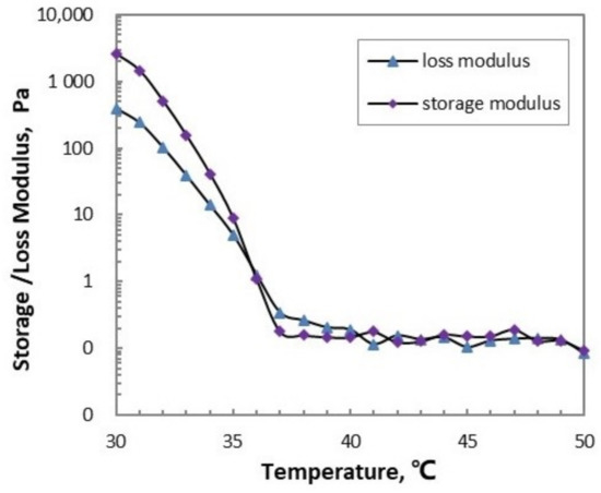
Figure 7.
Storage and loss moduli of the waxy crude oil varying with temperature.
3.4. Viscosity-Temperature Relation
Viscosities of the waxy crude oil sample were tested at every 5 C from 37 C down to 35 C with the rotational rheometer (Rheolab QS, Anton Paar, Graz, Austria). The pretreated oil sample was loaded in the rheometer which had been heated to 60 C for 15 min and then was cooled to each test temperature at a cooling rate of 0.5 C/min and stood still for 30 min. At each test temperature, viscometry was conducted under 3 different constant shear rate, 20 s, 50 s and 100 s. The measured viscosity was recorded every 5 min until the difference between two successive tested viscosities was below 5%, that is, until the steady state was achieved. The steady-state viscosities at all the test temperatures are presented in Table 1. From Table 1, one could see that the viscosities of different shear rates at each temperature above coincide, while the viscosity of different shear rates at 37 C have separated (not shown here), indicating the test temperatures between 40 C and 70 C are above the abnormal point, above which the flow behavior is completely Newtonian.

Table 1.
Newtonian viscosity at different temperatures, tested under different shear rates 20 s, 50 s, 100 s. Data provided by Zhang [12].
3.5. Rheological Flow Curves
The flow curves presented in Figure 1, relating shear stress to shear strain and to time t, were obtained with the coaxial cylinder sensor system of a controlled-stress rheometer (HAAKE RS 150,Karlsruhe, Germany). The oil sample was statically cooled from 60 C to the test temperature 34 C and stood for 2 h until steady gel structure formed. Then the rheometer was set to a constant shear rate (the actual shear rate will increase from zero to its set value with delay due to system inertia, though) 0.1 s and 1 s respectively, and the waxy oil gel is exposed under shear. As a particular stimulus for our work, we consider the flow curves and in the yielding region, corresponding to the shear strain range 0.001∼10.
4. Results
This section deals with the computing methods of the shear stress as a function of shear strain , or of time t, for different shear rate histories (or equivalently, for different input functions for . The connection between and comes from the dependence of on t, in such a way that we may give , or . Also, we will discuss an unusual finding related to the imposed shear rate history we encountered in analysing the experimental data. The evolution equations, material functions proposed in previous chapters are summarized in Section 4.2. Later, the parameters in each functions, both the directly and the indirectly obtained ones, are given respectively in Tables 3 and 4.
4.1. Imposed Shear Rate History
The input function on the boundary, that is, or as a function of time t, plays an influential role on the results of the model prediction. The different curves in Figure 4 are supposed to correspond to different constant values of , but it will always take some time to get the actual value of imposed shear rate to its set value , especially for the controlled-stress rheometers. And there might even be overshoots around the yielding point. In previous literature, this feature has only been briefly mentioned by Tracha et al. [11], and the influence of the particular history of still needs detailed investigation.
In experiments, the actual starts from a small value close to 0, and for a short time stays very low, when the gel has an infinite (or very high) viscosity. When yielding happens, viscosity reduces by several orders of magnitude within rather narrow strain interval, and the stress applied to the system suddenly becomes higher than the viscous resistance, so the shear rate will increase sharply around yield strain. Eventually, it will reach the time-independent set value imposed by the controlled-stress rheometer. The dynamical reasons for the delay and the overshoot might be inertia of the experimental device, and it will be examined in the future. Here, for the shear rate history under examination, the experimental curves of will be mathematically approached as a empirical equation
in which is a small initial, , phenomenological parameters controlling the increasing slope of the curve, and a relating to the overshoot value. If , Equation (16) predicts a shear rate history starting from and increasing smoothly without overshoot to its set value , whereas if , it predicts a overshoot in shear rate history.
To examine the role of shear rate plays in the model prediction, shear rate history with and without overshoot are both approximated with Equation (16). The values of the parameters are listed in Table 2 and the fitting results are presented in Figure 8. The dash line (color: navy blue) corresponds to shear rate history without overshoot, the solid line (color: light grey) to the shear rate history with overshoot, and the curve with discrete points (color: light blue) the observed one. The time evolution of shear strain could be obtained by integrating Equation (16) with respect to time t.
Table 2.
Values of parameters of the function Equation (16) for shear rate history.
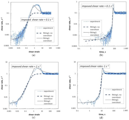
Figure 8.
Fitting curves of shear rate history with and without overshoot in comparison with measured ones: (a,b) for ; (c,d) for .
4.2. Summary of the Model
First, let us recall the evolution equation for stress in terms of the two material functions , , and the evolution equation for the structure parameter , which is given by the particular solution Equation (9) of Equation (7), and related to through the structural relation Equation (6). Thus, the model we have proposed in the above sections becomes
The input of the model is the shear rate described by Equation (21) with parameters listed in Table 2 in Section 4.1, whereas the output is the shear stress varying with time t, which is obtained in the experiment mentioned in Section 3.5. The time-, strain-dependent rheological variables necessary to obtain the output include the shear modulus given by Equation (18) and the viscosity , which may be obtained from Equation (19) along with Equation (20), in which is estimated to be 0.95 for , and 0.97 for by using Equation (12) and Equation (5).
Equation (17) will be solved by the finite-difference method to obtain evolution of stress
with the stress at time t.
4.3. Summary of the Parameters
The parameters of the presented model fall into two categories. Ones are rheological parameters with explicit physical meanings which can be directly measured or theoretically estimated under certain assumptions. Actually, their values are objective and are not supposed to be obtained through fitting process. The other category are the unknown parameters which are indirectly obtained through fitting of experimental curve, which in our case, is one of the curves for 0.1 s in Figure 1.
4.3.1. Directly Obtained Parameters
Five out of eleven parameters in the model may be obtained directly, including:
(1) The equilibrium elastic modulus of the relatively resistant network , the characteristic strains , in Equation (18); (2) Solvent viscosity in Equation (19); (3) The characteristic strain and D in Equation (10).
Among them, the characteristic strains and which are very much relevant to yielding are taken 0.25, according to the estimations of yield strain in Section 2.1.3. The equilibrium shear modulus of the resistent network is taken Pa, the equilibrium elastic modulus of Daqing crude oil at 34C as is tested in Teng and Zhang’s previous work [16]. We take the maximum packing volume fraction as Snabre and Mills [35,36] took. As for the fractal dimension of waxy crude gels, Yi and Zhng [44] obtained the box fractal dimension in experiments to be around 1.5, and thus it is taken here. In Section 5.4, we will take to see the consequences of different values fractal dimension.
For the solvent viscosity we employ an Arrhenius-type equation to extrapolate at test temperature from the experimental Newtonian viscosities at several different temperatures above WAT in Table 3. The parameters are and , obtained by fitting the experimental data. As a result, in the condition of the experiment is theoretically extrapolated to be 0.026 Pa·s (Figure 9).
Table 3.
Values of directly obtained parameters of the model.
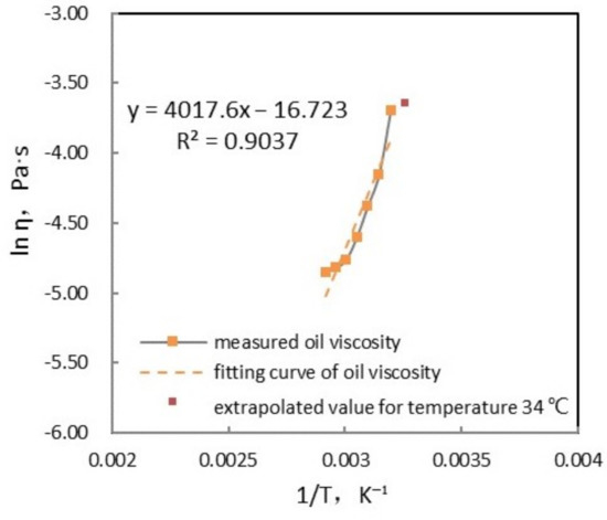
Figure 9.
Viscosity variation with temperature above wax appearance temperature (WAT) (experimental and ftting curves) and extrapolation of viscosity by Arrhenius equation, with parameters and .
4.3.2. Indirectly Obtained Parameters
The other category of indirectly obtained parameters includes 6 unknown parameters:
(1) , and , in Equation (18); (2) in Equation (19); (3) in Equation (20).
In this paper, we adjusted their values according to the flow curve in Figure 1a of the shear rate 0.1 s. Since these parameters are restricted to a certain range, rather than confined by certain objective values (at least the values could not be validated through experiments as far as we are concerned), they do not have to be taken the exact same values in all the figures corresponding to different conditions. The parameter values used in each figures in Section 5 are slightly different under the different conditions. The values used for the parameters of the main results in Figure 10 are the listed in Table 4, and others will be given under the each figure being discussed in next section. Compared to a numerical way, these fitting parameters are relatively rough estimations to help us get the main features of the proposed model under a given shear condition (yet it is satisfactory enough as will be shown in the following section). Note that the curves corresponding to have been predicted by using the same values obtained from the curve for . Their reasonable agreement with the observed curves of agreement with the observed curves of shows that our model is not only a fit of curves, but also has predictive capability.

Figure 10.
Fitting curves for shear rate and using the elastic modulus. model under the double-network assumption, and the shear rate history with inertial overshoot Equation (21) (with the fitting values in Table 2): (a) shear stress as a function of shear strain; (b) shear stress as a function of time.
Table 4.
Values of parameters estimated through rough fitting.
4.4. Fitting and Predicted Results: and
To obtain we use the evolution equation of Equation (17), in combination with expressions Equations (18) and (19) for the viscoelastic material properties, and Equation (20) for structure parameter. To examining the actual shear rate in the experiment, and to remove influence of the fluctuations in experimental data, we use the shear rate history with overshoot predicted by the empirical equation Equation (21). In Figure 10 the fitting curves for (red solid line) obtained by the model almost coincide with the experimental ones (red dotted lines).
The curves for are predicted by the model with the same parameters used to fit the curves, and are presented in Figure 10 with navy blue solid lines. The overall shapes of both and curves are of good analog with the measured ones (navy blue dotted line), especially in the pre-yielding region. The small deviation after yielding could be raised by the difference between the shear history described by the input function Equation (21) and the actual history. Moreover, it could be seen that the predicted yield stress is 39 Pa, 1 Pa less than the measured one, while the predicted yielding time is 10 s, same as the measured ones, both of which are quite satisfactory.
5. Discussion
From Section 2, Section 3 and Section 4, we present the theoretical justification from both microscopic and macroscopic prospective of the modelization of a nonlinear viscoelastic model used to describe the yielding of gelled waxy crude oil, and the experimental protocols used to obtain the data for model validation. The results of the model prediction shown in Figure 10 is found to be rather satisfactory. Several original aspects we have considered in modelling may have made a contribution: (1) the assumption of double-network gel; (2) the modification of the input shear history which deviates from the setting constant shear rate; (3) the employment of Marrucci’s viscoelastic model for the description of the stress evolution. In this section, we will plot the results of the model prediction in absence of the consideration of the above aspects and by comparing them with the results in Figure 10, the influence of each one of them will be evaluated respectively.
5.1. Double-Network vs. Single-Network Gel
In obtaining the theoretical curves in Figure 11, same calculation is used as in Figure 10, except that in Equation (18) is taken as 0 so that the gel is viewed as the conventional single network structure, and the value for the remaining network were changed to to fit the curve as much as possible. By comparing with experimental curves, the theoretical curves in Figure 10 obtained with the modulus model under the double network assumption (with an additional network whose elastic modulus is Pa, and characteristic shear strain is ) clearly exhibit a better description than the ones under the single network assumption.
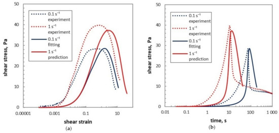
Figure 11.
Fitting curves for shear rate and of shear stress as a function of shear strain and of time, taking the whole calculation same as in Figure 10, but using the elastic modulus under the assumption of a single network structure by in Equation (18) and changing value for the remaining network to : (a) shear stress as a function of shear strain; (b) shear stress as a function of time.
Generally speaking, the main problem of the single-network elastic modulus model is that it results in a rather low stress before yielding. In Figure 11a, the curves for different imposed shear rates begin to separate at a strain of the order of 0.1, one order of magnitude higher than experimental curves. The fitting curve for reaches a maximum value equal to the experimental one, 30 Pa, while the predicted peak stress on the curve of reaches a peak stress 3 Pa lower than the experimental one. Also, the shear strains corresponding to the peak stresses for both the fitting curve and the predicted curve are more than one order of magnitude higher than the experimental ones. In Figure 11b, the curves show yielding times for both shear rates which are of the same order as experimental ones, with curve around 10 s and the curve around 100 s. But in the region before the stress peak, in both Figure 11a,b the predicted stresses are relatively small compared to the actual ones, so that the raise of the predicted curves is steeper than that of the experimental curves, while after the maximum value, the decreasing rates plotted with solid line are slower than the experimental ones.
5.2. Effect of the Non-Constant Input Shear Rate History
In Figure 12 and Figure 13, we explore the consequences of shear rate history, with all the parameters kept the same as in Figure 10. Rather than the actual shear rate history in experiments described by Equation (21), in Figure 13 we consider a constant shear rate and in Figure 12, we use a relaxational time history of shear rate without overshoot. This turns out to have relevant consequences. As we can see in Figure 13, the shapes of the curves change significantly upon using a constant shear rate input. Two most noticeable changes are, the small difference between the peak stress of different shear rate curves, and the very short yield times the model has predicted. This means that the fitness of previous models considered in the literature might be affected by the shear rate history, especially when the same type of rheometer (controlled-stress rheometer) is used. One problem of using the Maxwell-type stress equation is that the stress would have a non-zero initial value at time 0 s, as shown in Figure 13b, which however, does not agree with the experiments (discrete black points in Figure 8). With the inertial delay taken into account in Equation (21), this is no longer a limitation of the Maxwell-type model.
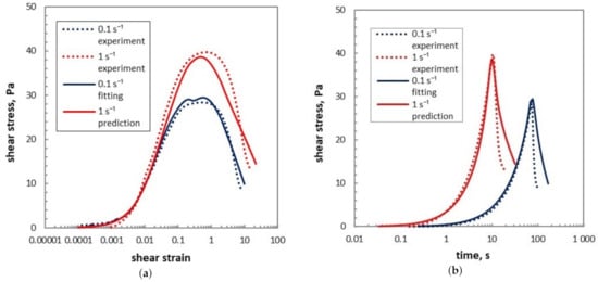
Figure 12.
Model predictions of shear stress as a function of shear strain and of time using a relaxational time history of shear rate Equation (21) (with the fitting values in Table 2: (a) shear stress as a function of shear strain; (b) shear stress as a function of time).
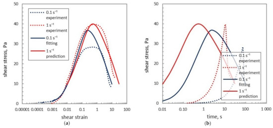
Figure 13.
Model predictions of shear stress as a function of shear strain and of time using constant shear rate without inertial delay: (a) shear stress as a function of shear strain; (b) shear stress as a function of time.
The curves in Figure 12a and the region below the stress peak in Figure 12b are satisfactory, whereas the decreasing rates of shear stress for both the fitting and predicted curves (plotted with solid lines) in Figure 12b are slightly higher than the corresponding experimental ones (plotted with dash lines). Also, the decreasing rate of the consequent curves at both shear rates are not as closer to the experimental one as those in Figure 10b. This comparison shows influence of the overshoot of input on the predicted curves.
5.3. Marrucci Model vs. Maxwell Model
In Figure 14, the curves are also obtained by using the same material functions Equations (14) and (10) as in Figure 10, and the same input shear rate history without overshoot described by function Equation (16), but instead of Marrucci’s non-linear viscoelastic model we have used the Maxwell viscoelastic equation . We use a different parameterization from that used to obtain Figure 10, by taking the value of equilibrium modulus Pa, , and others kept the same. As a result, although the yield stress for the fitting curve of 0.1 s is of the same order of the experiment alone, the height of the predicted curve of 1 s is far from the experimental ones. Moreover, the peak heights of the fitting and predicted curves (plotted with solid lines) are not to the scale as the experimental curves (plotted with dash lines). In Figure 14, the decreasing rate after yielding obtained by Maxwell model are unrealistically slow. Comparison of Figure 10 and Figure 14 shows the use of Marrucci’s model clearly improves the description of this situation. It is probably because the dynamics of shear modulus taken into consideration in Marrucci’s model has incorporated the thixotropic behavior of waxy gel and makes the description closer to its true mechanics.
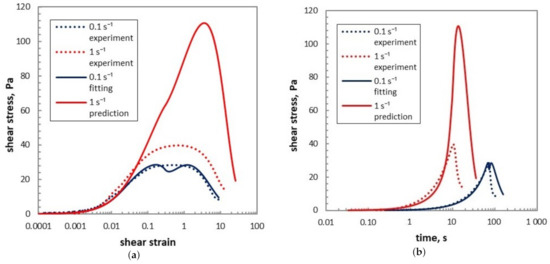
Figure 14.
Predictions of shear stress as a function of shear strain and of time with Maxwell viscoelastic model for stress instead of Marrucci model Equation (17): (a) shear stress as a function of shear strain; (b) shear stress as a function of time.
5.4. Effect of Fractal Dimension
Another factor to be considered related to structure is the value of the fractal dimension D. Generally speaking, fractal dimension is a parameter that may characterize the feature of the gel structure. The deviation of the value of fractal dimension from the dimension of Euclidean space D = 3 may be used as a measure for the complexity of the gel structure, which depends on the mechanism of aggregation. The actual value of fractal dimension found for waxy crude gel is often between 1.5 and 2.5 [40,44]. In the prediction results shown in Section 4.4, as well as in the anylasis in Section 5.1, Section 5.2 and Section 5.3, we have taken it as , which is noted in the literature as possible value of D[44]; here we compare it with the results obtained for . From Figure 15, we see that with lower fractal dimension assumed, the blob radius as well as the stress after yielding decrease faster with strain than curves for . The curves in Figure 15b share with Figure 10b and Figure 11b the steep uprise for between 1 and 10.
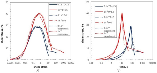
Figure 15.
Model predictions of shear stress as a function of shear strain and of time with taking fractal dimensions and : (a) shear stress as a function of shear strain; (b) shear stress as a function of time.
6. Conclusions
We have presented a simplified theoretical model for the yielding of a waxy crude oil by assuming the gel as a fractal structure. The predicted results of the model show a very close form in comparison with experimental curves. It gives a quantitative description of the isothermal nonlinear viscoelastic behavior of waxy crude gels formed under a given constant cooling rate, and may be used to estimate the minimum pressure and time needed to restart the flow after a period of shutdown. It has sufficient simplicity and wide flexibility to explore the influence of different physical factors, such as fractal dimension, shear rate history or the initial elastic modulus. Moreover, since we have not used any specific details of a waxy crude oil in the modeling process, the main framework of our model is sufficiently general to be also applicable to the yielding of other fractal gels.
Our model is based on evolution equations for stress and for structural parameter , and on a modelization for and . It starts from a definite physical model for the structure parameter instead of from more abstract parameterizations. Compared to previous works, five novel factors especially considered in our work have consequent advantages, namely: (1) the use of Marrucci’s nonlinear viscoelastic model in descriptions for the stress evolution; (2) The use of an explicit microscopic interpretation for the structure parameter in terms of the radius of the gel clusters, which allows us to estimate a range of the yield strain with simple arguments; (3) the material function for shear modulus G inspired by the double-network model; (4) the application of well-established sophisticated viscosity model to the description of the viscosity of a transient process; and (5) the modification the actual imposed shear rate history which deviates from the setting one due to device inertia.
Though the main framework of the model is very general, we have focused our attention on a concrete application. Further studies should be the following ones:
- (1) An extension to more values of nominal shear rate should be examined. Furthermore, applications to other typical rheometric situations such as oscillating shear and small-step increase of strain should also be carried out.
- (2) Physical grounds for the inertia effect of device as well as the double-network structure of elastic modulus still need further exploration. The empirical function Equation (21) for the actual shear rate history and the material function Equation (18) for the elastic modulus should be improved accordingly.
- (3) Based on the presented model developed for the yielding region and applied to a fixed temperature history and composition situation, a comprehensive description of the rheological behavior may be extended to. First, the composition and temperature dependence of the material functions should be studied to compare the predictions of the model in different circumstances. Secondly, the structural evolution needs to be understood microscopically, leading to a more detailed evolution equation on the basis of a rate function incorporating the build-up and destruction of structure.
Author Contributions
Conceptualization, M.S.; Formal analysis, M.S., D.J. and Z.W.; Funding acquisition, M.S.; Methodology, M.S. and D.J.; Software, M.S. and Z.W.; Validation, M.S. and Z.W.; Writing—original draft, M.S. and D.J.; Writing—review & editing, M.S., D.J. and Z.W. All authors have read and agreed to the published version of the manuscript.
Funding
This research was funded by the Foundation of China University of Petroleum (Beijing) for Start-up Research Programs grant number 2462017YJRC021, and the Strategic Cooperation Technology Projects of CNPC and CUPB grant number ZLZX2020-05.
Institutional Review Board Statement
Not applicable.
Informed Consent Statement
Not applicable.
Data Availability Statement
The data presented in this study are available in the article.
Acknowledgments
Conflicts of Interest
The authors declare no conflict of interest. The funders had no role in the design of the study; in the collection, analyses, or interpretation of data; in the writing of the manuscript, or in the decision to publish the results.
Abbreviations
The following abbreviations are used in this manuscript:
| DSC | Differncial Scanning Calormetry |
| WAT | Waxy Appearance Temperature |
| SAOS | Small amplitude oscillatory shear |
Appendix A. Estimation of the Yield Strain with Analytical Geometry

Figure A1.
Geometric graph of elongated of blobs.
We will use analytical geometry method to estimate the strain at the fracture (See Figure A1). The circle in the coordinate represents one of the blobs with its original shape and location before deformation, and the closed curve represents its status when flow begins. The origin of the coordinate is where the undeformed blob contacts its underneath neighboring blob. When a shear rate equal to is imposed on the blobs, the upper part will move faster than the lower part due to the gradient of velocity. Point O(0, 0) does not move during deformation, whereas point A (0, ), the top, moves . If the horizontal displacement of each point on circle is assumed to be proportional to its y-axis value, it will be translated with respect to the line . Assuming P(x, y) is any point on the circle, then we have
Equation (A1), which can be identified as an elliptic equation, would be the equation of the blob after deformation. If we move the center of the ellipse to the origin of the coordinate, its equation will become
Note that the equation of an origin-centered ellipse, with semi-major axis and semi-minor , rotated by angle has the following normalized form
By comparing the correspondent coefficient in Equations (A4) and (A5), one gets the following equation set
With the relation and the restriction condition , we eliminate , and in Equation (A6), and find the equation of as
Since the strain is rather small by the time of yielding, we neglect the high-order infinitesimals and , thus obtaining the approximate estimation of the critical shear strain .
References
- Rønningsen, H.P. Rheological behaviour of gelled, waxy North Sea crude oils. J. Pet. Sci. Eng. 1992, 7, 177–213. [Google Scholar] [CrossRef]
- Davidson, M.R.; Nguyen, Q.D.; Chang, C.; Rønningsen, H.P. A model for restart of a pipeline with compressible gelled waxy crude oil. J. Non-Newton. Fluid Mech. 2004, 123, 269–280. [Google Scholar] [CrossRef]
- Vinay, G.; Wachs, A.; Frigaard, I. Start-up transients and efficient computation of isothermal waxy crude oil flows. J. Non-Newton. Fluid Mech. 2007, 143, 141–156. [Google Scholar] [CrossRef]
- de Souza Mendes, P.R.; de Abreu Soaresa, F.S.; Zigliob, C.M.; Gonçalves, M. Startup flow of gelled crudes in pipelines. J. Non-Newtonian Fluid Mech. 2012, 179–180, 23–31. [Google Scholar] [CrossRef]
- Cheng, D.C.H. Yield stress: A time-dependent property and how to measure it. Rheol. Acta 1986, 25, 542–554. [Google Scholar] [CrossRef]
- Wardhaugh, L.T.; Boger, D.V. The measurement and description of the yielding behavior of waxy crude oil. J. Rheol. 1991, 35, 1121–1156. [Google Scholar] [CrossRef]
- Chang, C.; Boger, D.V.; Nguyen, Q.D. The yielding of waxy crude oils. Ind. Eng. Chem. Res. 1998, 37, 1551–1559. [Google Scholar] [CrossRef]
- Kane, M.; Djabourova, M.; Volle, J.L. Rheology and structure of waxy crude oils in quiescent and under shearing conditions. Fuel 2004, 83, 1591–1605. [Google Scholar] [CrossRef]
- Visintin, R.F.G.; Lapasin, R.; Vignati, E.; D’Antona, P.; Lockhart, T.P. Rheological Behavior and Structural Interpretation of Waxy Crude Oil Gels. Langmuir 2005, 21, 6240–6249. [Google Scholar] [CrossRef]
- Andrade, D.E.V.; da Cruz, A.C.B.; Franco, A.T.; Negrão, C.O.R. Influence of the initial cooling temperature on the gelation and yield stress of waxy crude oils. Rheol. Acta 2015, 54, 149–157. [Google Scholar] [CrossRef]
- Tarcha, B.A.; Forte, B.P.P.; Soares, E.J.; Thompson, R.L. Critical quantities on the yielding process of waxy crude oils. Rheol. Acta 2015, 54, 479–499. [Google Scholar] [CrossRef]
- Zhang, L. The Yield Properties of Gelled Waxy Crude Oil. Master’s Thesis, China University of Petroleum (Beijing), Beijing, China, 2011. [Google Scholar]
- Houska, M. Inzenyrske Aspekty Reologie Tixotropnich Kapalin. Ph.D. Thesis, Techn. Univ. Prague, Prague, Czech Republic, 1980. [Google Scholar]
- Doraiswamy, D.; Mujumdar, A.N.; Tsao, I.L.; Beris, A.N.; Danforth, S.C.; Metzner, A.B. The CoxMerz rule extended: Rheological model for concentrated suspensions. J. Rheol. 1991, 35, 647–685. [Google Scholar] [CrossRef]
- Jia, B.; Zhang, J. Yield behavior of waxy crude gel: Effect of isothermal structure development before prior applied stress. Ind. Eng. Chem. Res. 2012, 2012, 10977–10982. [Google Scholar] [CrossRef]
- Teng, H.; Zhang, J. A new thixotropic model for waxy crude. Rheol. Acta 2013, 52, 903–911. [Google Scholar] [CrossRef]
- Dullaert, K.; Mewis, J. A structural kinetics model for thixotropy. J. Non-Newton. Fluid Mech. 2006, 139, 21–30. [Google Scholar] [CrossRef]
- Teng, H.; Zhang, J. Rheological Behavior and Structural Interpretation of Waxy Crude Oil Gels. Ind. Eng. Chem. Res. 2013, 52, 8079–8089. [Google Scholar] [CrossRef]
- Mujumdar, A.; Beris, A.N.; Metzner, A.B. Transient phenomena in thixotropic systems. Ind. Eng. Chem. Res 2002, 102, 157–178. [Google Scholar] [CrossRef]
- Dimitrious, C.J.; McKinley, G.H. A comprehensive constitutive law for waxy crude oil: A thixotropic yield stress fluid. Soft Matter 2014, 35, 6591–6858. [Google Scholar] [CrossRef]
- Mewis, J.; Wagner, N.J. Thixotropy. Adv. Colloid Interface Sci. 2009, 147–148, 214–227. [Google Scholar] [CrossRef]
- Coussot, P.; Leonov, A.I.; Piau, J.M. Rheology of concentrated dispersed systems in a low molecular weight matrix. J. Rheol. 1993, 46, 179–217. [Google Scholar] [CrossRef]
- Yziquel, F.; Carreau, P.J.; Moan, M.; Tanguy, P.A. Rheological modeling of concentrated colloidal suspensions. J. Non-Newton. Fluid Mech. 1999, 86, 133–155. [Google Scholar] [CrossRef]
- Quemada, D. Rheological modelling of complex fluids: IV: Thixotropic and thixoelastic behaviour. Start-up and stress relaxation, creep tests and hysteresis cycles. Eur. Phys. J. Appl. Phys. 1999, 86, 191–207. [Google Scholar] [CrossRef]
- de Souza Mendes, P.R. Modeling the thixotropic behavior of structured fluids. J. Non-Newton. Fluid Mech. 2009, 164, 66–75. [Google Scholar] [CrossRef]
- de Souza Mendes, P.R. Thixotropic elasto-viscoplastic model for structured fluids. Soft Matter 2011, 7, 2471–2483. [Google Scholar] [CrossRef]
- de Souza Mendes, P.R.; Thompson, R.L. A unified approach to model elasto-viscoplastic thixotropic yield-stress materials and apparent yield-stress fluids. Rheol. Acta 2013, 52, 673–694. [Google Scholar] [CrossRef]
- Geest, V.C.B.G.C.V.D.; Merino-Garcia, D.; Bannwart, A.C. A modified elasto-viscoplastic thixotropic model for two commercial gelled waxy crude oils. Rheol. Acta 2015, 54, 545–561. [Google Scholar] [CrossRef]
- Mendes, R.; Vinay, G.; Ovarlez, G.; Coussot, P. Modeling the rheological behavior of waxy crude oils as function of flow and temperature history. J. Rheol. 2015, 59, 703–732. [Google Scholar] [CrossRef]
- Marrucci, G. The Free Energy Constitutive Equation for Polymer Solutions from the Dumbbell Model. Trans. Soc. Rheol. 1972, 16, 300–321. [Google Scholar] [CrossRef]
- Marrucci, G.; Titomanlio, G.; Sarti, G.C. Testing of a constitutive equation for entangled networks by elongational and shear data of polymer melts. Rheol. Acta 1973, 12, 269–275. [Google Scholar] [CrossRef]
- Acierno, D.; Mantia, F.P.L.; Marrucci, G.; Titomanlio, G. A non-linear viscoelastic model with structure-dependent relaxation times. I. Basic formulation. J. Non-Newton. Fluid Mech. 1976, 1, 125–146. [Google Scholar] [CrossRef]
- Acierno, D.; Mantia, F.P.L.; Marrucci, G.; Rizzo, G.; Titomanlio, G. A non-linear viscoelastic model with structure-dependent relaxation times. II. Comparison with l. D. polyethylene transient stress results. J. Non-Newton. Fluid Mech. 1976, 1, 147–157. [Google Scholar] [CrossRef]
- Acierno, D.; Mantia, F.P.L.; Marrucci, G. A non-linear viscoelastic model with structure-dependent relaxation times. II. Comparison with l. D. polyethylene transient stress results. J. Non-Newton. Fluid Mech. 1977, 2, 271–280. [Google Scholar] [CrossRef]
- Snabre, P.; Mills, P. I. Rheology of weakly flocculated Suspensions of rigid particles. J. Phys. III Fr. 1996, 6, 1811–1834. [Google Scholar] [CrossRef]
- Snabre, P.; Mills, P. II. Rheology of weakly flocculated Suspensions of viscoelastic particles. J. Phys. III Fr. 1996, 6, 1835–1855. [Google Scholar] [CrossRef]
- Dimitrous, C.J.; McKinley, G.H.; Venkatesan, R. Rheo-piv analysis of the yielding and flow of model waxy crude oils. Energy Fuels 2011, 25, 3040–3052. [Google Scholar] [CrossRef]
- Bautista, F.; de Santos, J.M.; Puig, J.E.; Manero, O. Understanding thixotropic and antithixotropic behavior of viscoelastic micellar solutions and liquid crystalline dispersions. I. The model. J. Non-Newton. Fluid Mech. 1999, 80, 93–113. [Google Scholar] [CrossRef]
- Lorge, O.; Djabourov, M.; Brucy, F. Crystallisation and gelation of waxy crude oils under flowing conditions. Rev. L’institut Français Pétrole 1997, 52, 235–239. [Google Scholar] [CrossRef]
- Gao, P.; Zhang, J.; Ma, G. Direct image-based fractal characterization of morphologies and structures of wax crystals in waxy crude oils. J. Phys. Condens. Matter 2006, 28, 11487–11506. [Google Scholar] [CrossRef]
- Hou, L. Experimental study on yield behavior of Daqing crude oil. Rheol. Acta 2012, 51, 603–607. [Google Scholar] [CrossRef]
- Venkatesan, R.; Ostlund, J.; Chawla, H.; Wattana, P.; Nyden, M.; Fogler, H.S. The effect of asphaltenes on the gelation of waxy oils. Energy Fuels 2003, 14, 1630–1640. [Google Scholar] [CrossRef]
- Soskey, P.R.; Winter, H.H. Equibiaxial Extension of Two Polymer Melts: Polystyrene and Low Density Polyethylene. J. Rheol. 1985, 29, 493–517. [Google Scholar] [CrossRef]
- Yi, S.; Zhang, J. Shear-induced change in morphology of wax crystals and flow properties of waxy crudes modified with the pour-point depressant. Energy Fuels 2011, 25, 5660–5671. [Google Scholar] [CrossRef]
Publisher’s Note: MDPI stays neutral with regard to jurisdictional claims in published maps and institutional affiliations. |
© 2021 by the authors. Licensee MDPI, Basel, Switzerland. This article is an open access article distributed under the terms and conditions of the Creative Commons Attribution (CC BY) license (http://creativecommons.org/licenses/by/4.0/).