Abstract
A two-way coupling particle flux model is proposed for studying the multi-component solid–fluid suspension. The suspension mixture is treated as a non-linear single-phase fluid and the migration of the solid particles is modeled by a particle flux equation. The proposed particle flux model takes the effects of the particle migration on the transport of the suspension’s momentum and internal energy into account. Two benchmark problems are calculated to study the performance of the proposed particle flux model, i.e., flow in a sudden expansion straight channel and flow between two rotating cylinders. It is found that the particle flux model converges without numerical stability issue with the commonly used PISO-SIMPLE transient solver, and the effect of the particle migration is evident on both velocity profile and temperature distribution.
1. Introduction
Solid–fluid suspensions are common in both engineering applications and geographic process. The transport of the particle sediments is fundamental for fluvial, estuarine and coastal morphology [1], sequestration processes in porous media [2], and formation of coal particle slurries with oil or water for coal feeders of power plants [3,4]. The rheological properties of these solid–fluid suspensions, such as the solid particles migration under flow, the viscosity and the heat transfer characteristics of the suspension mixture, are main issues affecting the successful operation of numerous engineering facilities [4,5,6].
For the flow of the solid–fluid suspension, when the density of the solid particles is remarkably larger than the density of the carrying fluid, particles sedimentation under gravity occurs. Such process could be studied numerically by the Computation Fluid Dynamics-Discrete Element Method (CFD-DEM) [7,8] and the two-fluid method [3,9,10], at the expense of added computational cost from the introduction of Lagrangian discrete phase or another fluid phase. A lower-cost variant takes the advantage of particle flux equation to model the effect of solid particles, so that both phases of the suspension could be calculated with single-phase transport equations. Compared with CFD-DEM and two-fluid method, the particle flux model typically has higher numerical stability, since only a scalar transport equation is added into the original Naiver–Stokes equations of the single-phase fluid. The advantage on numerical stability could be important for problems with complex geometry or extreme flow condition.
The most widely used particle flux method was proposed by Phillips et al. [11,12,13,14]. However, as a one-way coupling model, it considers only the effect of fluid on the motion of particles, the effect of the migration/transport of the solid particles back on the conservation of the linear momentum and internal energy are neglected. To address such effect, we derived a new particle flux model based on Phillips’ model [14], considering the effect of the particles migration/transport on the conservation of the linear momentum and internal energy of the fluid phase. The particle migration is completed using Phillips’ model with Tetlow’s empirical correlation [15]. Thermal diffusivity is formulated following Jeffery’s model, which considers the second order effects of thermal conductivity based on the solid volume fraction [4,16].
As the solid–fluid suspension typically shows complex non-linear rheological properties, it is important to properly model the constitutive relations within the stress tensor and heat flux. Although in some cases the solid–fluid suspension could be approximated by the Bingham or the Power law [17], under more common conditions the stress tensor strongly depends on the volume fraction of the solid component and the shear rate of the fluid flow. Krieger et al. [18] provided a general expression for the dependency of the viscosity on both solid volume fraction and shear rate. In addition, in applications such as the high speed bearing flow and deep sea drilling, the effect of by pressure and temperature on viscosity [4,5] must also be considered.
The paper is organized as follows: In the Methods section, the effect of the particle migration on the transport of the linear momentum and internal energy are investigated, based on Phillips’s model [14]. Then we introduce the constitutive equations for shear stress, heat flux and particles transport flux implemented in the proposed two-way coupling particle flux model. In the Results section, two benchmark problems are calculated by the proposed particle flux model and the results are discussed.
2. Methods
2.1. Governing Equations
For the conservation of mass, for both solid and fluid components based on the mixture theory
where , , and are the pure density of the fluid and the solid particle, in the reference configuration, therefore the mixture density is defined as; is the volume fraction of the solid particles, where . is the velocity of the suspension mixture. is the solid particle flux, which measures the transport/migration of the volume fraction of the solid component (for more details please refer to Equations (9) and (18)). Thus, and represent the mass transport of each component caused by the particle flux. Combining Equations (1) and (2), we can acquire
While the conservation of linear momentum can be written as
substituting Equations (1) and (2) into (5), we can acquire
In the current paper, we consider gravity as the only body force. Term is the linear momentum change caused by the particle flux .
As for the conservation of energy, following the previous derivation we have
where L is the gradient of velocity, q is the heat flux vector, is the mixture heat capacity and is the internal energy change due to the transport of the particle flux .
The conservation of solid concentration is simply
where is the particle diffusive flux.
2.2. Constitutive Equations
Roscoe [19] provided a thorough review of modeling and characterizing gel-like materials. In general, gels behave as non-Newtonian fluids (NNF). (Non-linear) NNF exhibit some unusual characteristics. For example, some NNF show normal stress effects, as manifested in phenomena such as die-swell or rod-climbing (see the book by Schowalter [20]). Some NNF have yield stress or show viscoelastic effects, while some have viscosities depending on shear rate and temperature or even pressure (see the books by Macosko [21], Carreau, De Kee and Chhabra [22]). Perhaps the simplest model, from an engineering perspective, which can capture the shear-thinning (or shear-thickening) effect, is the power-law model. In current work, for the shear stress tensor, we assume that the viscous stress of the solid–fluid suspension can be represented by a generalized power-law fluid model,
where is the volume fraction, is the turbulent eddy viscosity, is the reference suspending fluid viscosity, and is the shear dependency constant. In the above equations, depends on Krieger’s work which provides a correlation between the viscosity and particle concentration, formulated by both theoretical analysis and experimental data () [18]. represents the effect of volume fraction and shear-dependency. In current work, we assume that is a constant and predefined by the user.
The heat flux vector is modeled as follows:
where is the effective thermal conductivity. Various models are available to evaluate the effective thermal conductivity for solid–fluid suspensions [23,24,25], in current study we apply the model proposed by Jeffery [16], keeping consistent with our previous study [4]. Jeffery’s model considers the second order effects of thermal conductivity based on the solid volume fraction [26]:
where
and
For the constitution of particle flux, we do not take the Brownian motion into account since the size of the particles of interest is sufficiently large. Then, the diffusive particle flux becomes
where , , and are the flux due to particles collision, spatial variations in the viscosity, gravity and turbulence, respectively.
Following Phillips’ model [14], particle flux due to collisions and non-uniform viscosity are evaluated as
where a is the characteristic particle length (e.g., radius), is the local shear rate, is the effective viscosity, and are empirically determined coefficients. According to Phillips et al. [14], accounts for the effect of the spatially varying interaction frequency due to the collision between particles, while accounts for the effect of the spatially varying viscosity. Mathematically and are responsible for the particles migrations causing non-homogenous distribution of the particles. Seifu et al. [27] noted that the particle flux could be given as . We could see that is a field potential incorporating mechanisms that cause migration of particles. Phillips et al. and Subia et al. [6,14] assumed that , are constants. In this paper, we apply the empirical correlation proposed by Tetlow et al. [15]
As for the gravity-induced particle flux, based on the work of Acrivos et al. [28] and Mavromoustaki [11], could be modeled as
where
This gravity flux model has been applied to various studies, such as falling of thin film [11]. For other mathematical models of gravity induced particle flux, please refer to [1,29].
The particle flux due to turbulence reads
where is the eddy viscosity and is the Schmidt number which is assumed as 0.9 for current study [30,31].
By substituting the Equations (10) and (11) into (6), (12)–(15) into (8), and (16)–(23) into (9), we obtain a set of expanded governing equations for the particle flux model. For the expanded form of governing equations based on the original Phillips’s model [7], please refer to Appendix A.
Conservation of mass:
Conservation of linear momentum:
Conservation of energy:
Conservation of particles concentration:
3. Results and Discussion
To evaluate the performance of the two-way coupling particle flux model, two benchmark problems were calculated and analyzed in this chapter—namely, the flow in straight sudden expansion channel and the flow between two rotating cylinders (circles). The simulation results would also be compared with the original Phillips’ model [14]. Numerical simulation of both benchmark problems was finished by a user-defined solver developed based on the open sourced CFD toolbox OpenFOAM [16]. The NS equation was solved by the standard PISO-SIMPLE (so-called PIMPLE) algorism, a transient segregated solver iterating between pressure and velocity to enforce mass conservation over momentum equations. The pressure-velocity iteration would be renewed to the next time step should initial (normalized) residual of pressure was lower than and that of the velocity was lower than . During the transient calculations, the maximum Courant (maxCo) number was kept below 0.9 everywhere in the flow filed, to resolve the time-dependent information [32].
For spatial discretization, central difference (CD) interpolation was used for gradient and Laplacian terms, while convection terms were interpolated by a so-called “bounded Gauss linear” scheme, which improve the boundedness of the simulation by taking advantage of the incompressible part of velocity divergence term (non-zero before convergence was reached). For temporal discretization, implicit Euler scheme was applied for time derivative terms. As both cases were wall bounded flow, Wilcox’s k-omega model was used for the treatment of turbulence effect, and coefficients were chosen according to [33]. The underlying assumption of unsteady Reynolds-averaged Navier–Stokes (URANS) turbulence method was that the local turbulence scale estimated by RANS is sufficiently smaller than the dominating large-scale fluctuation [34,35,36,37,38,39]. Standard wall functions were applied for turbulence variables such as k (turbulent kinetic energy) and omega (specific dissipation of k) on all solid walls, where no-slip and zero gradient boundary conditions were used for velocity and pressure, respectively. The value of the gravity , was set as a constant value of . To reduce computational cost of transient simulation, both calculations were performed on two-dimensional (2D) grid(s). It was acknowledged that the three-dimensional dynamics of vortices stretching could not be captured by 2D grid with URANS turbulence treatment. The purpose of the benchmark calculation served essentially as a test on the model performance and its numerical stability, by comparison with the original Phillips’s model. When the local small transient scale was not dominant or not the major interest of the study, the computationally cheaper 2D calculation could also provide valuable information, especially for the testing of the new model and numerical method [40,41].
3.1. Flow in Straight Sudden Expansion Channel
Figure 1 and panel (a) of Figure 2 showed the computational grid and geometry of the straight sudden expansion channel. The inlet velocity was 0.5 , and the inlet volume fraction of the solid component was 0.05. The radius of particle was 1 . Temperature of the inlet flow was set as 393 , as the suspending fluid was water, laminar viscosity was set as a constant of 1 in accordance with the temperature. The density of the suspending fluid and the solid particles were 1000 and 3000 . As a result, if we used half the step height at the sudden expansion as the reference length scale, corresponding hydraulic Reynolds would be , verifying the application of turbulence model. The mass heat capacity of the water was set as 4023 . To enhance the effect of the particle flux on the fluid temperature, we assumed a high heat capacity for the particles, which was equal to that of the carrying water. On all solid walls, temperature was kept constant at 293 . For the initial condition of the solid phase, velocity, temperature and solid volume fraction were 0 , 293 and 0, respectively. It should be pointed out that to demonstrate the path of the particles sediment, the gravity body force would not take effect until the sudden expansion, in other words, there was no gravity in the inlet channel before the sudden expansion.
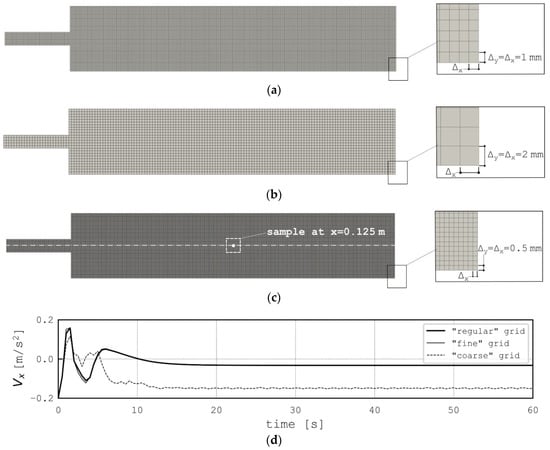
Figure 1.
Computational grid used for grid independence validation. (a) grid used for calculation & analysis; (b) “coarse” grid which doubled the step size compared with the grid used; (c) “fine” grid which halved the step size compared with the grid used; (d) evolutions of velocity sampled at the geometry center of expanded channel.
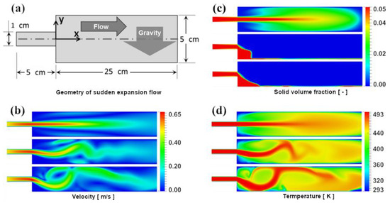
Figure 2.
(a) Schematic of the straight sudden expansion channel; (b) The velocity distribution; (c) The volume fraction distribution of the solid particles; (d) The temperature distribution. For the panel (b–d), from top to bottom the three different fields are simulation results by: 1. Phillips’ model [14] without considering gravity; 2. Phillips’ model [14] considering the gravity; 3. Proposed particle flux model considering gravity. All the fields are the acquired at t = 2 s.
Governing equations of the suspension was discretized by a 2D structured grid, a constant spatial resolution of 1 1 was applied throughout the entire flow domain, as shown in Figure 1, and from then on it would be referred to as the “regular” grid or simply the “grid used”. To confirm grid independence of solution, simulation was conducted with different levels of spatial resolutions. Two of them could be found in Figure 1, namely a “coarse” and “fine” grid, as the corresponding step size was 2 and 0.5 , respectively. Calculations on all three grids converged reasonably without numerical stability issues. Additionally, the velocity in the X direction () was sampled at the geometric center of the expanded channel, namely at the location (x = 0.125, y = 0). As shown in panel (d) of Figure 1. In fact, for the “fine” and “regular” grid, both velocity profile and solid volume fraction distribution converged into quasi steady state after flow time (t) = around 20 s, due to the strong diffusion effect of RANS turbulent model. However, velocity profile of the “coarse” grid calculation kept oscillating, even the ensemble mean value was quite different from the predictions of finer grid, as shown in Figure 1d. As refining the “regular” grid brought little difference on the simulation results, we assumed that the evenly distributed 1 mm step size was sufficient for current study, at least in terms of grid independency. The discussions of analysis of the simulation results were based on the “regular” grid. For a more detailed verification study of the numerical setup, please check Appendix B.
Simulation was performed for 60 s of flow time for all the cases with different parameters, for both the new particle flux model and the original Phillips model, total wall-clock times were around s (~2.8 h) on a dual-channel machine with DDR4 DRAM clocked at 3200 MHz. The reason was that in typical CFD calculations, bottleneck of computation workload was the iteration between p-U coupling, especially the pressure equation, so the extra equations introduced by the new particle flux model brought little CPU overhead.
Panel (b), (c) and (d) of Figure 2 showed the velocity, solid volume fraction and temperature fields after t = 2 s. Inside each panel, the top contour showed the simulation results using the original Phillips’ model [14] but without considering the gravity; the middle contour represents results by Phillips’ model [14] considering the gravity effect; while simulation results of the proposed particle flux model considering the gravity effect were displayed in the bottom contour. According to the top contours of all the three panels, we could see that when Phillips’s model [14] was applied and gravity was neglected, all fields were symmetric along the channel symmetric line. Whereas when gravity body force was considered by Phillips’ model [14], in other words, when there is gravity but the effect of the particle flux on the fluid was ignored, particles sediment near the bottom wall was obvious after the sudden expansion, which also slightly modified the velocity and temperature profiles. However, as shown in the bottom contours of panel (b), (c) and (d), when the effect of the particle flux on the fluid was also considered (namely applying the proposed particle flux model), the high velocity and high temperature region shifted substantially towards the particles sediment direction. One explanation could be that the settling particle carried the momentum and the temperature from center region towards the bottom wall, so that the particle flux enhanced the convection of momentum and heat transfer. More interestingly, if one looked at the volume fraction field shown in panel (c), it could be found that the proposed two-way coupling particle flux model predicted a streamlined particles sediment shape, the solid component moves more like a projectile motion. Such streamlined shape of the particles sediment should be attributed to the different velocity field predicted by the proposed model, which estimated higher convection rate of momentum transfer from the high-speed center region to the bottom part of the channel.
Figure 3, Figure 4 and Figure 5 showed the evolution of the velocity, solid volume fraction and temperature fields, predicted by the proposed two-way coupling particle flux model with gravity considered. From the first 1 to 3 s, the high-velocity region gradually moved towards the direction of the gravity. At 20 s, the velocity field was almost fully developed. Along the flow direction, the high velocity region firstly leaned towards the bottom wall after the expansion, and then climbed towards the opposite direction, induced by the evolution of volume fraction distribution. It could be found that almost all the solid particles settled down rapidly near the bottom wall, as shown in Figure 2c and Figure 4c. This should be related to the large particle size and density difference between the particles and suspending fluid. Furthermore, Figure 4 showed that as the flow evolved, the particles sediment region kept growing along the flow direction. Within the first 3 s, the sediment region maintained a streamlined shape, while as the front of the sediment was pushed further away from the inlet, the tailing slope of the interface between the sediment and suspending fluid becomes steeper. This could be explained as that the settled particles far away from the sudden expansion were transported from the surface of the upstream sediment rather than settling down from the main stream of the flow (by gravity effect). The temperature profiles of the suspension, as displayed in Figure 5, evolved towards a more uniform distribution during the process of sedimentation. The temperature distribution in the bottom corner, in particular, is even more uniform compared with the rest of flow domain, due to the effect of the particle flux.
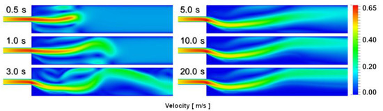
Figure 3.
The velocity fields at different time steps with considering the gravity and using the proposed particle flux model.
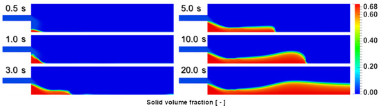
Figure 4.
The volume fraction fields of the solid component at different time steps with considering the gravity and using the proposed particle flux model.
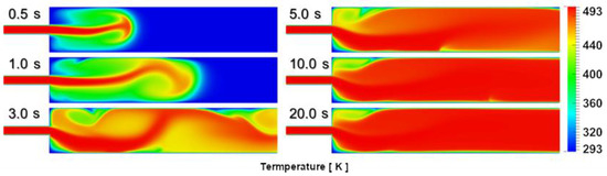
Figure 5.
The temperature fields at different time steps with considering the gravity and using the proposed particle flux model.
3.2. Flow between Two Rotating Cylinders (Circles)
In this section, the performance of the proposed particle flux model was evaluated by another benchmark problem: flow between two rotating cylinders. This problem was quite common in engineering applications, such as the bearing flow and the well drilling flow in the oil and geothermal industry. Figure 6 showed the geometry of the two cylinders. The radius of the inner and the outer cylinders were 0.64 and 2.54 , respectively. The inner cylinder was rotating at 180 RPM and the outer cylinder is static. The kinetic viscosity of the suspending fluid was set as , leading to a hydraulic Reynolds number around , so the entire flow region could be regarded as fully developed turbulence [42,43,44]. The temperature of the outer cylinder and the inner cylinder were 393 K and 293 K, respectively. To speed up the simulation, firstly a steady state calculation was carried out without considering the motion of either fluid or solid, then the temperature profile of the steady state solution was used as the initial condition of transient calculation. The initial velocity of transient calculation is 0 , and the initial solid volume fraction is 0.1. The gravity was along negative Z-direction. The other parameters and flow conditions were kept unchanged with the previous case.
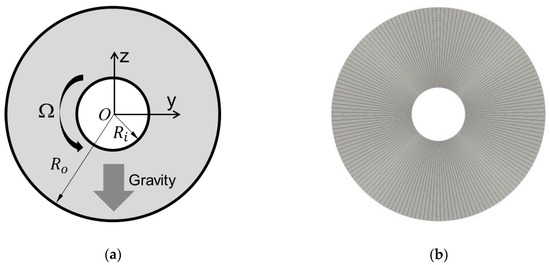
Figure 6.
Geometry and computational grid of the two concentric cylinders.
A fully structured O-grid was used for calculation. As no special refinement was applied to the boundary layer, bunching of grid layers in both radial and circumferential direction was equally divided. To contain computational cost, grid dependence study similar to the previous section was performed, and spatial resolution was chosen so that further refinement would not improve the simulation results. As the results, typical grid step size was set to be 1 in the near wall region of outer cylinder, hence near the inner cylinder wall it was around 0.4 , the total cell count was around 12,000. The transient simulation converged to a quasi-steady state after around 1 s of flow time (t = 1 s), and the calculation was continued until t = 12 s. For both proposed particle flux model and original Phillips model, total wall-clock times were around 4000 s on the same dual-channel machine used for simulation of sudden expansion flow, due to the same reason that the extra equations introduced by the new particle flux model were not the bottleneck of computation workload.
Figure 7 showed the velocity, solid volume fraction and temperature distribution after t = 0.2 s, the top panels represented the results predicted by the Phillips’ model [14], while the bottom panels represented the results by the proposed two-way coupling model. In fact, for the solid volume fraction distribution, the results by two different models were quite similar, although the effect of the particle flux could still be observed for the temperature and velocity fields, particularly around the inner cylinder.
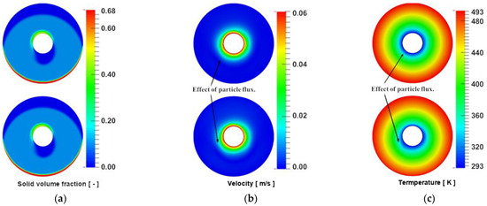
Figure 7.
The flow fields at t = 0.2 s. (a) Volume fraction of the solid particles; (b) Velocity distribution; (c) Temperature distribution. The top panels represent the results predicted by Phillips’ model [14], the bottom panels represent the results predicted by the proposed particle flux model.
Figure 8, Figure 9 and Figure 10 show the evolution of velocity, solid volume fraction and temperature fields at different time steps. From Figure 8, we can see that as flow time increases, the solid particles migrated towards the bottom wall of the outer cylinder. Due to the effect of the rotation of the inner cylinder, the particles settling on the top wall of the inner cylinder was not symmetric along the y direction and those particles moved gradually towards the bottom of the outer cylinder. We might infer that if the inner cylinder was static, the time required to complete the particle sediment towards the bottom of the outer cylinder would be much longer. Figure 9 shows an obvious effect of the particle sediment on the velocity field. Near the inner cylinder, the high velocity region always corresponded to the high concentration of the solid particles where the viscosity also took high values. Figure 10 shows the temperature evolution with the increasing of flow time. Near the top wall of the outer cylinder, the high temperature region was slightly shifted towards the direction of gravity, as shown in Figure 10 for t = 0 s and t = 1 s. This could be attributed to the enhancement of heat transfer termed from the particle flux, which was strongly controlled by the force of gravity due to density difference between solid and fluid.
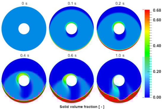
Figure 8.
Volume fraction of the solid component at different time steps predicted by the proposed particle flux model.
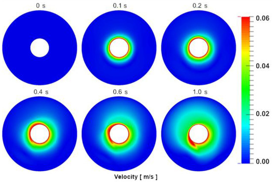
Figure 9.
Velocity field at different time steps predicted by the proposed particle flux model.
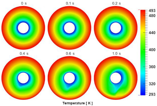
Figure 10.
Temperature fields at different time steps predicted by the proposed particle flux model.
4. Conclusions
The particle flux model by Phillips et al. [14] was further developed so that a two-way coupling particle flux equations—namely, the particle flux model could be formulated by considering the effect of the particle migration on the transport of the momentum and internal energy of the fluid phase. The proposed two-way coupling particle flux model manifested reasonable numerical stability during the calculation of two benchmark problems, whose results indicated that the effect of the particle migration on the flow and heat transfer was evident; hence, in a situation where the density of a particle is sufficiently higher than the suspending fluid, it is expected that the proposed model could provide more reasonable prediction than one-way coupling models. Further extension of the application to three-dimensional process with more complex geometry is expected though, as the proposed particle flux model brought almost no additional computational cost. Besides, although solution verification showed that the numerical methods behaved as expected in terms of estimated error and observed order, carefully designed experimental validation for more flow conditions should be carried out for further calibration and development of the proposed particle flux model.
Author Contributions
Y.W. performed all the simulations and prepared the manuscript; W.-T.W. developed the mathematical model and revised the paper. Both authors have read and agreed to the published version of the manuscript.
Funding
This research received no external funding.
Institutional Review Board Statement
Not applicable.
Informed Consent Statement
Not applicable.
Data Availability Statement
Data is contained within the article.
Conflicts of Interest
The authors declare no conflict of interest.
Appendix A
Here we provide the expanded form of the governing equations based on model proposed by Phillips et al. [14].
Conservation of mass:
Conservation of linear momentum:
Conservation of particles concentration:
Conservation of energy:
Appendix B
Solution verification was conducted by systematic grid refinement, following “Performance Test Code Committee PTC-61” [45]. Freitas suggested that at least 3 different grid resolutions must be tested to achieve a convincing error estimation, we used 5 of them, since the proper resolution was not known a priori. As shown in Table A1, verification started from a quite coarse grid (#5, in fact the “coarse” grid in Figure 1), with grid step size around 2 , while the grid #1 has the finest grid spacing of 0.5 (the “fine” grid in Figure 1). Although it was not mandatary, we followed the suggestion of Freitas to keep steady refinement factors between neighbor grids, which were chosen to approximate 1.4 (square root of 2).

Table A1.
Grids parameters for error estimation.
Table A1.
Grids parameters for error estimation.
| No (#i) | Grid Spacing (h) | Refinement Factor (r) | Factor of Safety (Fs) |
|---|---|---|---|
| #5 | 2 | 1.4 | 1.25 2 |
| #4 | 1.43 | 1.43 | 1.25 |
| #3 1 | 1 | 1.4 | 1.25 |
| #2 | 0.71 | 1.42 | 1.25 |
| #1 | 0.5 | \ | 1.25 |
1 The grid used for calculation & analysis; 2 Value of Fs were suggested by [45,46].
To access the solution error, was sampled on 4 different points alone the symmetric line. As shown in Figure A1, sampled points were evenly distributed along the x direction. A direct comparison of the sampled velocities were displayed in Figure A1, the reported flow time was t = 2 s, when the difference between prediction by gird (#3) and that of the “fine” grid (#5) reached its maximum value, as shown in panel (d) of Figure 1. If we take the grid used (#3) as the reference to define the spatial refinement ratio (r*), it could be found that solution results were quite grid dependent when the value r* was lower than 0.75, whereas refinement beyond r* = 1 brought little difference on the simulation results, as shown in Figure A1.

Figure A1.
Location of sample points for error estimation (solution verification). L is the length of expanded channel in x direction.
Figure A1.
Location of sample points for error estimation (solution verification). L is the length of expanded channel in x direction.

The visual trend of progress reported in Figure A1 was the primitive reason for the choice of grid #3 to access the model performance. For a more complete solution verification, error estimation must be performed to calculate the extrapolated error and observed order of the method. As the largest discrepancy between predictions of different grid resolution came from the sample point near the inlet channel (line with circle marker in panel (a) of Figure A2), we used at sample point x = 0.2 L to calculate error and observed order, following the 3-grid procedure defined in [45].

Figure A2.
Prediction of on sample points resolution at flow time = 2 s by (a) grids with different spatial refinement ratio and (b) same grid with different temporal refinement ratio.
Figure A2.
Prediction of on sample points resolution at flow time = 2 s by (a) grids with different spatial refinement ratio and (b) same grid with different temporal refinement ratio.

Two groups of “3-grid”, namely Group A {#3, #4, #5} and Group B {#2, #3, #4}, were used to calculate the estimated error, so that a more convincing grid independence validation could be quantified. The results were reported in Table A2, namely the observed order (p), extrapolated values (ϕ21ext), relative error (ea21), estimated extrapolated relative error eext21, and the fine grid convergence index GCIfine21 of the numerical setup adopted in current work. Please refer to PTC-61 [45] for the complete definition and calculation steps. Although it was not surprising to see quite an unusual high value of observed order for Group A due to the poor prediction by grid #5, it proved that neither grid #5 nor #4 suffice to provide any meaningful analysis, at least based on current numerical setup. In the meantime, the observed order of 1.23 from grids in Group B was a much more reasonable value, since the numerical schemes adopted were not purely 2nd order. The observed order and estimated error, along with the value cascade shown in Figure A2, were evidences that the simulation series by three grids in Group B were in the asymptotic region, so that grid #3 could be regarded as the cheapest choice for calculation and further analysis.
Table A2.
Sample uncertainty analysis by different spatial resolution.
Table A2.
Sample uncertainty analysis by different spatial resolution.
| Group | N11 | N2 | N3 | r21 | r32 | p | ϕ21ext | ea21 | eext21 | GCIfine21 |
|---|---|---|---|---|---|---|---|---|---|---|
| A | 25,480 | 13,000 2 | 6370 | 1.4 | 1.43 | 9.01 | 0.1549 | 1.53% | 0.07% | 0.09% |
| B | 52,000 | 25,480 | 13,000 2 | 1.43 | 1.4 | 1.23 | 0.1506 | 1.02% | 1.92% | 2.35% |
1N stands for the total cell count of the grid; 2 N of grid used for calculation & analysis.
Similar procedure was performed using different sets of time steps on the same grid (#3), by adjusting the maximum allowed Courant number (maxCo). Following the definition of spatial refinement ratio, the temporal refinement ratio (rt*) was defined using maxCo = 0.9 as the reference. E.g., for calculation with maxCo controlled below 0.45, the value of rt* is 2. Again two groups of different rt* were calculated, Group I included cases where the series of rt* equaled {1, 0.5, 0.25}, whereas for Group II it was {2, 1, 0.5}. The results were summarized in Table A3. For both groups of rt*, the observed order was low than 1, mainly due to implicit Euler scheme adopted for time derivative terms, although it should be pointed out that the observed orders by the refinement of temporal and spatial resolution should not be interpreted in an identical way (due to initial residual control of PISO-SIMPLE algorithm). Since the sample point chosen represent almost the worst scenario of the simulation, and maxCo lower than 1 is the widely used criteria even for standard PISO algorism (without initial residual control) [47], the upper limit of 0.9 for the maxCo was regarded as a balance between a cost-effective method and insuring a level of accuracy.
Table A3.
Sample uncertainty analysis by different temporal resolution.
Table A3.
Sample uncertainty analysis by different temporal resolution.
| Group | C11 | C2 | C3 | r21 | r32 | p | ϕ21ext | ea21 | eext21 | GCIfine21 |
|---|---|---|---|---|---|---|---|---|---|---|
| I | 0.9 2 | 1.8 | 3.6 | 2 | 2 | 0.50 | 0.1757 | 3.29% | 7.35% | 9.9 % |
| I 3 | 0.9 2 | 1.8 | 3.6 | 2 | 2 | 1 3 | 0.1682 | 3.29% | 3.19% | 4.12 % |
| II | 0.45 | 0.9 2 | 1.8 | 2 | 2 | 0.62 | 0.1728 | 2.10% | 3.80% | 4.93% |
| II 3 | 0.45 | 0.9 2 | 1.8 | 2 | 2 | 1 3 | 0.1698 | 2.10% | 2.06% | 2.63% |
1C stands for maxCo allowed during simulation; 2 maxCo adopted for calculation & analysis; 3 using a forced observed order of 1, as suggested in [45].
As the both benchmark problems were calculated with 2D grid, one fair question would be that a 3D calculation should be applied instead. Since the additional dimension would dramatically increase the simulation time, one case of 3D calculation was performed based on the proposed model, as shown in Figure A3. Span width in the z direction was set to be equal to the height in the y direction, while the 3D grid employed the same spatial resolution as the “regular” 2D grid (#3 in Table A1). Cyclic boundary condition was applied for the patches normal to the z direction, so the suspension could be regarded as flow in an infinitely wide channel. All the other setups were kept identical to the 2D calculation.
Velocity fields were sampled on 2 planes normal to the z direction, namely the first symmetric plane where z = 0, and the plane close to the boundary where z = −0.4 of the width of the channel (Lz in Figure A3). Figure A4 compared the sampled results with the 2D calculations at t = 2 s and t = 25 s. It was found that the prediction of 3D calculation was quite similar with that of the 2D calculation, due to the cyclic boundary condition and the strong diffusion effect of URANS turbulence model adopted. As mentioned in the Results and discussion section, although being limited by the incapability to track the 3D vortices stretch process of turbulence, the 2D URANS calculation could still provide valuable information for a preliminary performance evaluation of the proposed model.

Figure A3.
Geometry and grid of 3D calculation.
Figure A3.
Geometry and grid of 3D calculation.


Figure A4.
Velocity profiles of at (a) t = 2 s; (b) t = 25 s. From top to bottom the contours are the simulation results of 3D grid sampled at plane z = 0, 3D grid sampled at plane z = −0.4 Lz, and the “regular” 2D grid.
Figure A4.
Velocity profiles of at (a) t = 2 s; (b) t = 25 s. From top to bottom the contours are the simulation results of 3D grid sampled at plane z = 0, 3D grid sampled at plane z = −0.4 Lz, and the “regular” 2D grid.

References
- Hsu, T.-J.; Traykovski, P.A.; Kineke, G.C. On modeling boundary layer and gravity-driven fluid mud transport. J. Geophys. Res. Space Phys. 2007, 112, 04011. [Google Scholar] [CrossRef]
- Ingber, M.S.; Graham, A.L.; Mondy, L.A.; Fang, Z. An improved constitutive model for concentrated suspensions accounting for shear-induced particle migration rate dependence on particle radius. Int. J. Multiph. Flow 2009, 35, 270–276. [Google Scholar] [CrossRef]
- Wu, W.-T.; Aubry, N.; Massoudi, M. On the coefficients of the interaction forces in a two-phase flow of a fluid infused with particles. Int. J. Non-Linear Mech. 2014, 59, 76–82. [Google Scholar] [CrossRef]
- Wu, W.-T.; Massoudi, M. Heat Transfer and Dissipation Effects in the Flow of a Drilling Fluid. Fluids 2016, 1, 4. [Google Scholar] [CrossRef]
- Zhou, Z.; Wu, W.-T.; Massoudi, M. Fully developed flow of a drilling fluid between two rotating cylinders. Appl. Math. Comput. 2016, 281, 266–277. [Google Scholar] [CrossRef]
- Subia, S.R.; Ingber, M.S.; Mondy, L.A.; Altobelli, S.A.; Graham, A.L. Modelling of concentrated suspensions using a continuum constitutive equation. J. Fluid Mech. 1998, 373, 193–219. [Google Scholar] [CrossRef]
- Cundall, P.A.; Strack, O.D.L. A discrete numerical model for granular assemblies. Géotechnique 1979, 29, 47–65. [Google Scholar] [CrossRef]
- Su, J.; Gu, Z.; Xu, X.Y. Discrete element simulation of particle flow in arbitrarily complex geometries. Chem. Eng. Sci. 2011, 66, 6069–6088. [Google Scholar] [CrossRef]
- Rajagopal, K.R.; Tao, L. Mechanics of Mixtures; Series on Advances in Mathematics for Applied Sciences; World Scientific: Singapore, 1995; Volume 35. [Google Scholar]
- Johnson, G.; Massoudi, M.; Rajagopal, K. Flow of a fluid—Solid mixture between flat plates. Chem. Eng. Sci. 1991, 46, 1713–1723. [Google Scholar] [CrossRef]
- Mavromoustaki, A.; Bertozzi, A.L. Hyperbolic systems of conservation laws in gravity-driven, particle-laden thin-film flows. J. Eng. Math. 2014, 88, 29–48. [Google Scholar] [CrossRef]
- Armanini, A.; Dalrì, C.; Fraccarollo, L.; Larcher, M.; Zorzin, E. Experimental analysis of the general features of uniform mud-flow. In Proceedings of the 3rd International Conference on Debris-Flow Hazards Mitigation: Mechanics, Prediction, and Assessment, Davos, Switzerland, 10–12 September 2003; Volume 1, pp. 423–434. [Google Scholar]
- Wang, L.; Mavromoustaki, A.; Bertozzi, A.L.; Urdaneta, G.; Huang, K. Rarefaction-singular shock dynamics for conserved volume gravity driven particle-laden thin film. Phys. Fluids 2015, 27, 033301. [Google Scholar] [CrossRef]
- Phillips, R.J.; Armstrong, R.C.; Brown, R.A.; Graham, A.L.; Abbott, J.R. A constitutive equation for concentrated suspensions that accounts for shear-induced particle migration. Phys. Fluids A Fluid Dyn. 1992, 4, 30–40. [Google Scholar] [CrossRef]
- Tetlow, N.; Graham, A.L.; Ingber, M.S.; Subia, S.R.; Mondy, L.A.; Altobelli, S.A. Particle migration in a Couette apparatus: Experiment and modeling. J. Rheol. 1998, 42, 307–327. [Google Scholar] [CrossRef]
- Jeffrey, D.J. Conduction through a random suspension of spheres. Proc. R. Soc. Lond. Ser. A Math. Phys. Sci. 1973, 335, 355–367. [Google Scholar] [CrossRef]
- Macosko, C. Rheology: Principles, Measurements and Applications; Wiley-VCH Inc.: New York, NY, USA, 1994; ISBN 1560815795. [Google Scholar]
- Krieger, I.M. Rheology of monodisperse latices. Adv. Colloid Interface Sci. 1972, 3, 111–136. [Google Scholar] [CrossRef]
- Roscoe, R. Suspensions, flow properties of disperse systems. In Flow Properties of Disperse Systems; North Holland Publishing Company: Amsterdam, The Netherlands, 1953. [Google Scholar]
- Schowalter, W.R.; Lumley, J.L. Mechanics of Non-Newtonian Fluids. Phys. Today 1980, 33, 57. [Google Scholar] [CrossRef]
- Macosko, C.W.; Larson, R.G. Rheology: Principles, Measurements, and Applications; Wiley: Hoboken, NJ, USA, 1994. [Google Scholar]
- Carreau, P.J.; De Kee, D.C.R.; Chhabra, R.P. Rheology of Polymeric Systems: Principles and Applications; Hanser Pub Inc.: New York, NY, USA, 1997. [Google Scholar]
- Maxwell, J.C. A Treatise on Electricity and Magnetism, 2nd ed.; Clarendon Press: Oxford, UK, 1873. [Google Scholar]
- Hamilton, R.L.; Crosser, O.K. Thermal Conductivity of Heterogeneous Two-Component Systems. Ind. Eng. Chem. Fundam. 1962, 1, 187–191. [Google Scholar] [CrossRef]
- Lu, S.; Lin, H. Effective conductivity of composites containing aligned spheroidal inclusions of finite conductivity. J. Appl. Phys. 1996, 79, 6761–6769. [Google Scholar] [CrossRef]
- Batchelor, G.K.; O’Brien, R.W. Thermal or electrical conduction through a granular material. Proc. R. Soc. Lond. Ser. A Math. Phys. Sci. 1977, 355, 313–333. [Google Scholar] [CrossRef]
- Seifu, B.; Nir, A.; Semiat, R. Viscous dissipation rate in concentrated suspensions. Phys. Fluids 1994, 6, 3189–3191. [Google Scholar] [CrossRef]
- Acrivos, A.; Mauri, R.; Fan, X. Shear-induced resuspension in a couette device. Int. J. Multiph. Flow 1993, 19, 797–802. [Google Scholar] [CrossRef]
- Abedi, M.; Jalali, M.A.; Maleki, M. Interfacial instabilities in sediment suspension flows. J. Fluid Mech. 2014, 758, 312–326. [Google Scholar] [CrossRef]
- Van Rijn, L.C. Sediment Transport, Part II: Suspended Load Transport. J. Hydraul. Eng. 1984, 110, 1613–1641. [Google Scholar] [CrossRef]
- Amoudry, L.O.; Hsu, T.; Liu, P.L. Schmidt number and near-bed boundary condition effects on a two-phase dilute sediment transport model. J. Geophys. Res. Space Phys. 2005, 110, 110. [Google Scholar] [CrossRef]
- Issa, R. Solution of the implicitly discretised fluid flow equations by operator-splitting. J. Comput. Phys. 1986, 62, 40–65. [Google Scholar] [CrossRef]
- Wilcox, D.C. Turbulence Modeling for CFD; DCW Industries: La Cañada Flintridge, CA, USA, 1998; Volume 2. [Google Scholar]
- Paredi, D.; Lucchini, T.; D’Errico, G.; Onorati, A.; Pickett, L.; Lacey, J. Validation of a comprehensive computational fluid dynamics methodology to predict the direct injection process of gasoline sprays using Spray G experimental data. Int. J. Engine Res. 2020, 21, 199–216. [Google Scholar] [CrossRef]
- Casimir, N.; Xiangyuan, Z.; Ludwig, G.; Skoda, R. Assessment of statistical eddy-viscosity turbulence models for unsteady flow at part and overload operation of centrifugal pumps. In Proceedings of the 13th European Conference on Turbomachinery Fluid Dynamics and Thermodynamics, Lausanne, Switzerland, 8–12 April 2019. [Google Scholar]
- Sadiki, A.; Maltsev, A.; Wegner, B.; Flemming, F.; Kempf, A.; Janicka, J. Unsteady methods (URANS and LES) for simulation of combustion systems. Int. J. Therm. Sci. 2006, 45, 760–773. [Google Scholar] [CrossRef]
- Hasse, C. Scale-resolving simulations in engine combustion process design based on a systematic approach for model development. Int. J. Engine Res. 2015, 17, 44–62. [Google Scholar] [CrossRef]
- Musa, O.; Chen, X.; Li, Y.; Li, W.; Liao, W. Unsteady Simulation of Ignition of Turbulent Reactive Swirling Flow of Novel Design of Solid-Fuel Ramjet Motor. Energies 2019, 12, 2513. [Google Scholar] [CrossRef]
- Li, W.; Chen, X.; Cai, W.; Musa, O. Numerical Investigation of the Effect of Sudden Expansion Ratio of Solid Fuel Ramjet Combustor with Swirling Turbulent Reacting Flow. Energies 2019, 12, 1784. [Google Scholar] [CrossRef]
- Wu, Z.; Cao, Y. Numerical simulation of airfoil aerodynamic performance under the coupling effects of heavy rain and ice accretion. Adv. Mech. Eng. 2016, 8, 168781401666716. [Google Scholar] [CrossRef]
- Schmid, P.J. Dynamic mode decomposition of numerical and experimental data. J. Fluid Mech. 2010, 656, 5–28. [Google Scholar] [CrossRef]
- Lathrop, D.P.; Fineberg, J.; Swinney, H.L. Turbulent flow between concentric rotating cylinders at large Reynolds number. Phys. Rev. Lett. 1992, 68, 1515–1518. [Google Scholar] [CrossRef] [PubMed]
- Brandstater, A.; Swinney, H.L. Strange attractors in weakly turbulent Couette-Taylor flow. Phys. Rev. A 1987, 35, 2207–2220. [Google Scholar] [CrossRef]
- Babkin, V.A. Fully Developed Turbulent Taylor–Couette Flow. J. Eng. Phys. Thermophys. 2014, 87, 1505–1512. [Google Scholar] [CrossRef]
- Freitas, C.J. Verification and Validation in Computational Fluid Dynamics and Heat Transfer: PTC 61. In Proceedings of the ASME 2006 Power Conference, Atlanta, GA, USA, 2–4 May 2006; pp. 793–800. [Google Scholar]
- Roache, P.J. Verification and Validation in Computational Science and Engineering; Hermosa Albuquerque: Hermosa Beach, CA, USA, 1998; Volume 895. [Google Scholar]
- Ferziger, J.H.; Perić, M.; Street, R.L. Computational Methods for Fluid Dynamics; Springer International Publishing: Cham, Switzerland, 2020; ISBN 978-3-319-99691-2. [Google Scholar]


Publisher’s Note: MDPI stays neutral with regard to jurisdictional claims in published maps and institutional affiliations. |
© 2021 by the authors. Licensee MDPI, Basel, Switzerland. This article is an open access article distributed under the terms and conditions of the Creative Commons Attribution (CC BY) license (http://creativecommons.org/licenses/by/4.0/).