Hazards Generated by an LNG Road Tanker Leak: Field Investigation of Vapour Propagation under Class B Conditions of Atmospheric Stability

Abstract

The publication presents the results of a field test of 2–4 min releases of 96% LNG from a road tanker designed to carry the gas. The release was performed at a pressure of 5.9–6.1 atm at a discharge rate of 1.67–1.78 kg/s from a height of 0.75 m under class B conditions of atmospheric stability. Comparison of the obtained experimental results of the maximum concentrations and the simulation carried out with the EFFECS (11.2.0) software showed that the Gaussian gas model better describes the gas cloud propagation at most control points at this release intensity than the dense gas model. The dense gas model gave only slightly better results along the cloud propagation axis at close distances, not exceeding 25/30 m at ground level. It is shown that concentrations between 71% and 110% LEL are observed at the cloud visibility limit. The maximum value of the temperature drop, in the release axis, at a distance of 4 m amounts to ∆T_max = 93.3 °C. This indicates that the cloud of the released LNG is almost entirely in the vapour state already in the short distance from the point of release, due to the turbulent outflow of the pressurised gas.

1. Introduction

LNG is one of the most important commodities used in the industry. An estimated 354.7 MT of LNG was traded in 2019, increasing by 13% over 2018 [1]. This growth will continue to be seen due to the undeniably numerous advantages of LNG, particularly in the environmental context. This is because methane, which is its main component in the combustion process, generates the least amount of incomplete combustion products of all hydrocarbon fuels, due to its lowest carbon content and the highest content of hydrogen, respectively. However, growing LNG trade is associated with an increased likelihood of uncontrolled releases, particularly during road transport. From the point of view of safety, transport is the factor most difficult to control due to dispersion and lower technological regime compared with industrial plants. Hence, hazards related to transport are of greatest interest to emergency responders due to the possibility of incidents occurring at any point in the road or rail network. The fact that 14.3% of all fires in 2018 were transportation fires attests to the frequency of transport-related hazards [2]. Another important issue is that, more often than not, local emergency responders, the least prepared to handle gas incidents, will be the first to come into contact with the gas during uncontrolled transport releases.

Estimation of vapour propagation in the case of LNG and determination of fire and explosion hazard zones is a rather severe problem which has been analysed by multiple researchers [3,4,5,6,7,8,9,10,11,12,13,14,15,16,17,18]. This is because gas cloud propagation is a result of the behaviour of dense gas and passive gas, depending on the type of LNG, the magnitude of the release, the current atmospheric conditions and the associated class of atmospheric stability, the pressure and temperature of the discharge, the type of substrate, or the turbulence during the release [3]. Therefore, it is very difficult to obtain reproducible experiment conditions in the field, even if this is merely in the aspect of maintaining stable atmospheric conditions. The vapour density in relation to air for the main component of LNG (methane) is temperature dependent. Before the gas becomes passive, starting from the boiling point (−161 °C) up to some −120 °C, the gas cloud tends to creep near the surface of the substrate. In this range, its density is greater than the density of the air at the standard normal ambient conditions (0 °C, 1013 hPa)—including in the release temperature after phase transition—by some 1.5 times [3]. Hence, the initially cold gas cloud has a tendency to creep and is not very susceptible to dissipation, especially at low wind speeds [3,4]. Large field tests have demonstrated this with significant LNG release rates, especially the Burro 8 test [3,17,18,19,20]. The cloud behaviour conforms to the dense gas model while being significantly wider and spread over a much larger area than predicted by the Gaussian gas model of passive dispersion. In some cases, such as the Burro 8 test mentioned above, the cloud may split into two parts [3]. However, at low release volumes, the cloud diluted with air masses disperses rapidly and heats up very quickly at a short distance from the release point. The basis for evaluating cloud propagation includes the estimation of the Richardson number, which represents the ratio of the potential energy associated with the excess density of a dense gas cloud to the kinetic energy of atmospheric turbulence [10,21]. However, Gaussian gas models and integral dense gas models do not give a complete answer as to the propagation of the cloud, especially in the presence of obstacles [3,10]. Hence, many fitting attempts, based mainly on CFD modelling, have been described in the literature in order to map the propagation of gas clouds, especially for large releases of the gas [3,4,5,6,7,8,9,10,11,12,13,14,15,16,17,18]. In contrast, there is relatively little research and analysis concerning smaller releases, despite the fact that such events occur much more frequently, and their effects can be significant [3,22,23].

2. Materials and Methods

2.1. Testing the Concentration of Flammable Gases in the Cloud Formed after the LNG Release

As part of the field tests, 4 series of combustible gas concentration tests were conducted using an array of 30 explosimeters that record the concentration, stationary at a given location, as a function of time. Two additional explosimeters were moved along the border of the visible gas cloud. The article presents only those measurement series for which it was possible to maintain stable wind conditions, particularly in wind direction. Recordings were made by averaging the measurements over minute or half-minute intervals, recording against methane. GfG999E wireless multi-gas detectors were used for the measurements giving the ability to measure CH₄ concentration from 0 to 100%. Releases lasting two–four minutes occurred during the morning hours of a summer day under class B conditions of atmospheric stability. The prevailing atmospheric and release conditions are presented in

Table 1. Ambient and LNG release parameters during the 4 test runs. Designations: Q—LNG discharge rate; T_a—ambient temperature; T_LNG—LNG temperature; P_a—atmospheric pressure; t—release time; p_out—release pressure; u_w—wind speed m.s⁻¹.

Series	Q, kgs−1	Ta, °C	TLNG, °C	uw, ms−1	Pa, hPa	t, s	pout, atm
1	1.67 ± 0.11	19.2	−162	0.89 ± 0.09	1003.0	120	6.0 ± 0.1
2	1.72 ± 0.14	20.1	−162	0.73 ± 0.13	1002.8	144	6.0 ± 0.1
3	1.70 ± 0.08	20.3	−162	0.67 ± 0.12	1002.7	163	5.9 ± 0.1
4	1.78 ± 0.10	20.7	−162	0.57 ± 0.16	1002.8	243	6.1 ± 0.1

. A schematic representation of the sensor placements in each test run is shown in Figure 1. To measure the prevailing atmospheric conditions, a Delta Ohm HD32.1 microclimate meter was used, along with a set of probes, to measure individual parameters. The gas release was performed at an intensity of 1.67–1.78 kg/s from an LNG road tanker, equipped with a spill hose with a diameter of d = 40 mm. In the study, the so-called light LNG, containing 96% CH₄, 3.6% ethane, 0.3% propane, and 0.1% butane was used. The temperature at the end of the hose line was −162 °C. Medium was released due to the pressure generated by the road tanker’s pump in the pressure range of 5.9–6.1 atm. The release occurred from a height of h = 0.75 m.

Based on the molar fraction dependence of liquid and gas fractions as a function of temperature for this type of LNG, presented by Laciak et al., it can be assumed that the LNG leaving the road tanker was entirely in the liquid phase [24]. However, liquid spill formation was practically not observed. Before the LNG released from the set height reached the ground level, there was an almost instantaneous phase transition of the LNG—after leaving the hose—due to the turbulent outflow of high-pressure fluid (Figure 2). In this case, the confirmation of turbulent fluid outflow is the high Reynolds number Re > 50,000 (Re = 4Q/pdn ≈ 4 × 10⁵, where: n—kinematic viscosity of methane (m²s⁻¹); Q—discharge rate (kg·s⁻¹); d—medium density (kg·m⁻³); p—pressure (Pa)).

2.2. Determination of Ambient Temperature Drop during LNG Release

A schematic representation of the test rig used to determine the ambient temperature drop during LNG release is presented in Figure 3. The coordinates of the thermocouples (x;y;h), expressed in metres, are shown in

Table 2. Coordinates of thermocouples (x;y;h) and their distance from the gas stream axis.

Thermocouple Number	Coordinates (x;y;h), m	Dist. from the Gas Stream Axis L, m
T1	(0;0;0.75)	0
T2	(2;0;0)	0.75
T3	(2;1;0.75)	1
T4	(2;−1;0.75)	1
T5	(2;−1;1.5)	1.25
T6	(2;1;1.5)	1.25
T8	(4;−1;0.75)	1
T9	(4;0;0.75)	0
T10	(4:1;0.75)	1
T11	(4;−1;1.5)	1.25
T12	(4;1;1,5)	1.25
T8	(4;−1;0.75)	1

. The LNG hose outlet was located at point T1 with the coordinates (0;0;0.75). The measurements used a 16-channel temperature recorder WRT-16M with an operating temperature range up −200 °C. Readings were taken in a separate measurement series at the following parameters: 1: Q = 1.71 kg/s, T = 21.3 °C, v = 0.52 m/s, RH = 47%, p = 1001.9 hPa. Release parameters: p_out = 6 atm, t = 75 s, h = 0.75 m.

2.3. Simulation Software

The experimental values obtained were related to the gas dispersion simulations performed in the EFFECTS software (11.2.0). In addition, a comparison of experimental values to theoretical simulations was made using both the Gaussian gas dispersion model based on the Yellow Book (CPR-14E) and the dense gas dispersion model. In the latter case, a SLAB-type model developed by the Lawrence Livermore National Laboratory was used.

In the case of the Gaussian gas model, dispersion of the medium is determined by atmospheric turbulence, which is a function of stability of the atmosphere and the height above the ground. The state of the atmosphere is not affected by the presence of substances in the air. Assuming that distribution of wind speed is homogeneous, it can be stated that the distribution of substances in a small cloud takes the Gaussian shape. The basic output formula of the passive dispersion (Gaussian plume model), in the case of continuous release, is described by Formula (1), as follows:

$$c(x,y,z)=\frac{q}{2\pi ·u_a{\sigma }_y{\sigma }_z}·\exp \left(-\frac{y^2}{2{\sigma }_y^2}\right)·\exp \left(-\frac{{(H-z)}^2}{2{\sigma }_y^2}\right)$$

(1)

where:

c(x,y,z)—concentration in (x,y,z) coordinate (parts per unit volume)

q—mass flow rate (kg·s⁻¹)

u_a—ambient wind velocity (m·s⁻¹)

σ_y—cross-wind dispersion parameter of cloud (m)

σ_z—vertical dispersion parameter of cloud (m)

H—cloud centre line (m)

x—down-wind horizontal coordinate (m)

y—cross-wind horizontal coordinate (m)

z—vertical (upward) coordinate (m)

A detailed mathematical description of the Gaussian gas dispersion model is presented in Chapter 4.5 of the Yellow Book [25].

The propagation of heavy gas is described by Navier–Stokes differential equations for density and instantaneous velocity fields. Averaged equations form an independent set of velocity, temperature, density, and concentration fields. Calculations used in EFFECTS software (11.2.0) are based on the SLAB model, first developed by ZEMAN, which introduced the concept of a one-dimensional shallow layer model [25]. The computational mechanisms implemented by the program assume the Gaussian distribution of a gas in vertical and horizontal cross-sections. In the three-dimensional SLAB model for continuous release, the concentration for any point in the space c(x,y,z) can be expressed by Formulas (2)–(6), shown below:

$$c(x,y,z) = 2b_y{b}_{z}c(x)·F_y(y,y_b,C_y)·F_z(z,H,{\sigma }_z)$$

(2)

$$c(x)=\frac{{\mu }_{a}m(x)}{{\mu }_s+({\mu }_a-{\mu }_s)m(x)}$$

(3)

$$F_y(y,y_b,C_y)=\left[erf\frac{y+y_b}{1.414C_y}-erf\frac{y-y_b}{1.414C_y}\right]/4y_b$$

(4)

$$F_z(z,H,{\sigma }_z)=\left[\exp (-\frac{{(z-H)}^2}{2{\sigma }_z^2}+\exp (-\frac{{(z+H)}^2}{2{\sigma }_z^2}\right]/\sqrt{2\pi {\sigma }_z^2}$$

(5)

$$c_y^2=0.33(b_y^2-y_b^2)$$

(6)

where:

c(x)—average volume concentration (parts per unit volume)

F_y(y,y_b,C_y)—spacial distribution function for lateral dispersion

F_z(z,H,σ_z)—spacial distribution function for vertical dispersion

y_b and C_y—shape parameters, related to each other by Formula (5)

μ_a—molar weight of dry air (kg·mol⁻¹)

μ_s—molar weight of dispersing material (kg·mol⁻¹)

b_y—half-width of the cloud in cross-wind direction (m)

b_z—cloud height (m)

A detailed mathematical description of the SLAB model is also presented in Chapter 4.5 of the Yellow Book [25].

Calculations in EFFECTS (11.2.0) software were made for pure methane. In order to calculate the cross-wind dispersion parameter (σ_y), the averaging time t_av = 30 s and the exponent value 0.2 were assumed. The adopted value allows meeting the requirement that the correction factor C_t should have a value of at least 0.5, so not less than that corresponding to the instantaneous release. In calculation of σ_y and σ_z, the parameters for class B atmospheric stability from Chapter 5.4.3.4 of the Yellow Book was used [25].

The stability of the atmosphere was determined based on the Pasquill and Smith scheme, based on wind speed, cloud cover, temperature, and time of day. The value of latitude of the position of the earth was adopted for Warsaw and it amounts to φ = 52.237°. Surface roughness length was assumed for the flat land at z₀ = 0.03 m. Based on Laciak’s work and temperature measurements, the initial liquid mass fraction equal to 1 was adopted [24].

2.4. Statistical Measures Used in Results Elaboration

The following statistical performance measures (SPMs) were selected to determine the extent to which the experimental results obtained matched the values obtained during the simulation:

(a)

Mean Relative Bias (MRB)

MRB can be described by Formula (7), as follows:

$$MRB=〈\frac{(C_m-C_p)}{0,5(C_m-C_p)}〉$$

(7)

where:

C_m—concentration obtained in the experiment

C_p—concentration predicted by the simulation

MRB accepts zero values and is not sensitive to low values. It is considered verified when the C_m/C_p ratio is not greater than 10, which will satisfy the presented tests. The measure is symmetric for both overestimated and underestimated values obtained from the simulation.

(b)

FAC2 Fraction of Prediction Within A Factor Of Two Measurements

FAC2 can be described by the following simple relationship 0.5 ≤ C_p/C_m ≤ 2

FAC2 tells us whether the difference between the predicted and experimental values is higher than the factor of 2.

(c)

Geometric Mean Bias (MG)

MG can be described by Formula (8), as follows:

$$MG=\exp 〈\ln \left(\frac{C_m}{C_p}\right)〉$$

(8)

MG has the advantage of reducing the impact of outliers. However, it does not accept zero values.

(d)

Geometric Variance (VG)

VG can be described by Formula (9), as follows:

$$VG=\exp 〈{\left[\ln \left(\frac{C_m}{C_p}\right)\right]}^2〉$$

(9)

As with MG, the associated VG has the advantage of reducing the impact of outliers. However, it does not accept zero values.

The adequacy of values predicted by dispersion models has been the subject of multiple analyses [10,26,27]. Based on the research of the Hanna team, and taking into account possible uncertainties, the range proposed by 59 A standards of National Fire Protection Association (NFPA) was adopted, according to which, the following ranges of statistical measures corresponding to a good dispersion model should be satisfied: −0.4 < MRB < 0.4; 0.5 ≤ C_p/C_m ≤ 2; 0.67 < MG < 1.5; VG < 3.3 [10,25].

3. Results

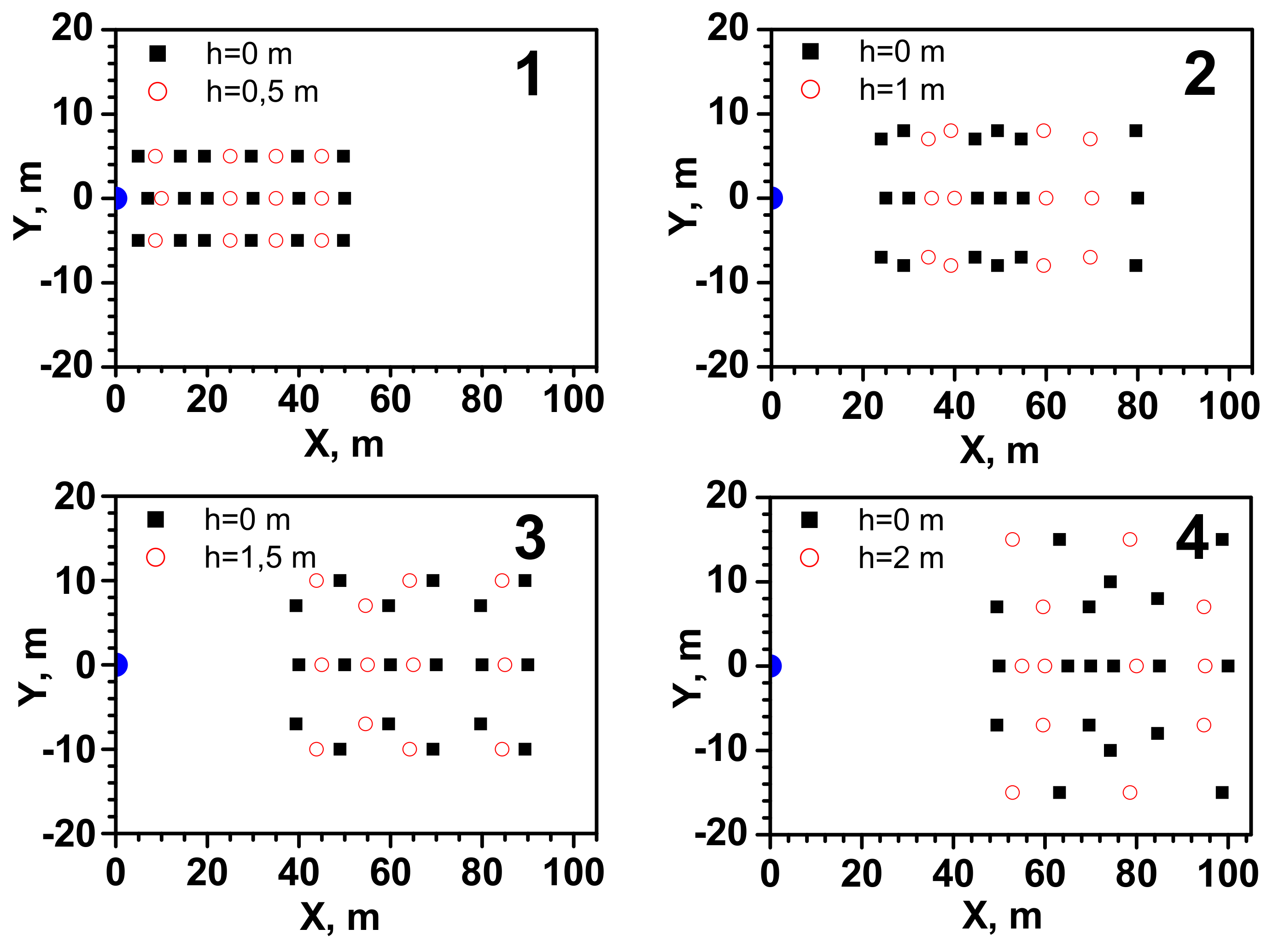
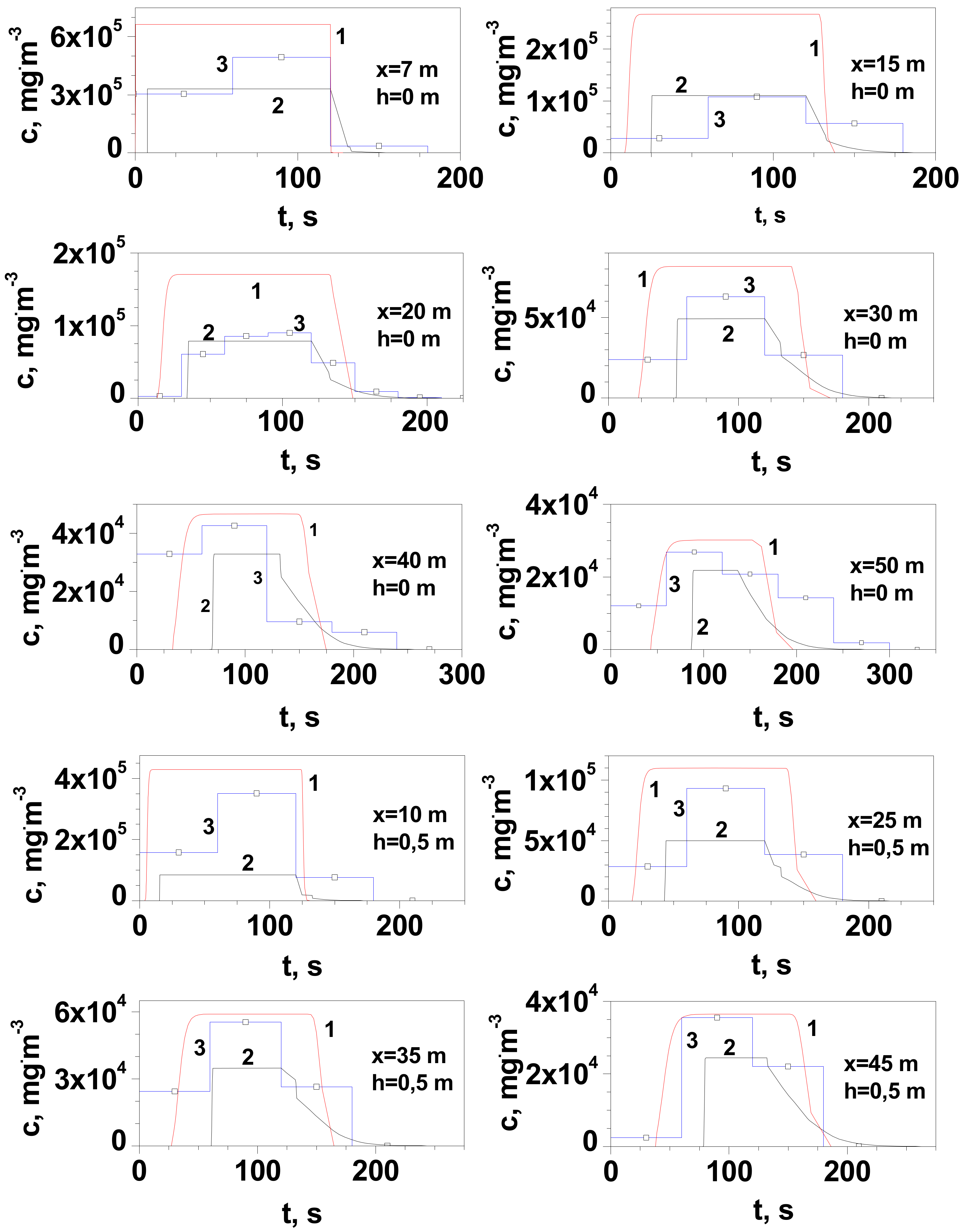
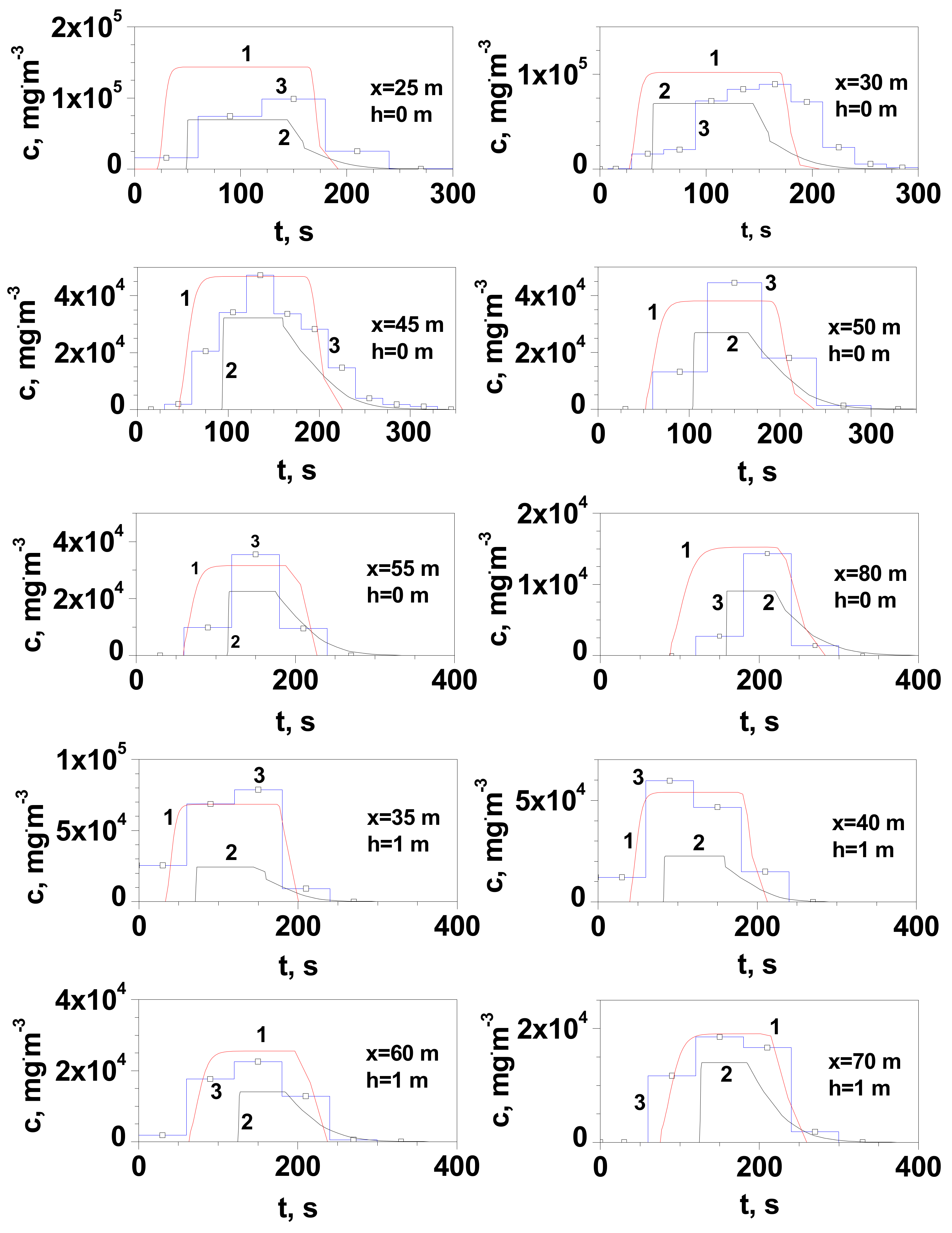
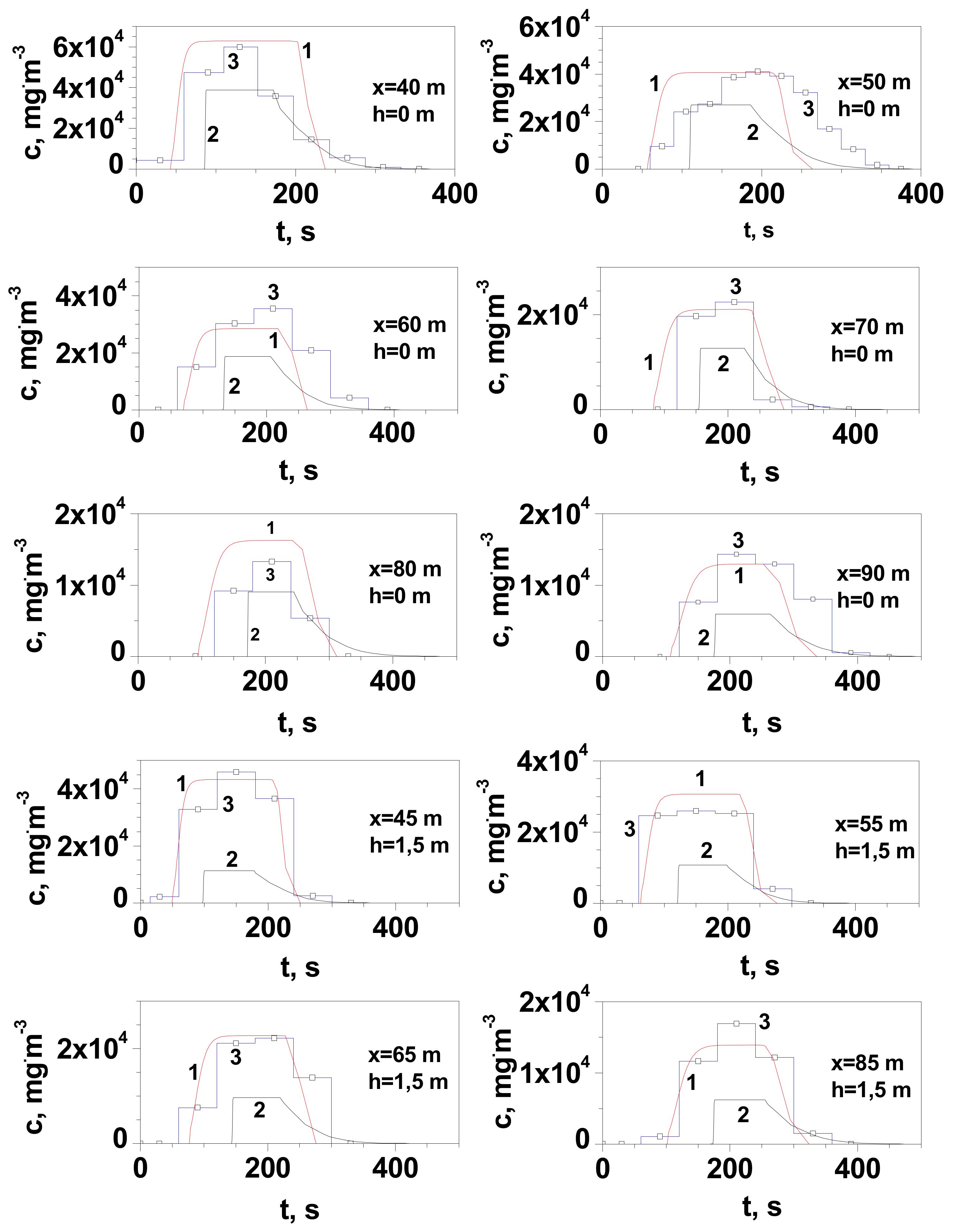
3.1. Results of Testing the Flammable Gas Concentration in the Cloud Formed after the LNG Release

The comparison of the concentration dependence as a function of time for the calculated values, according to the Gaussian gas model and the dense gas model, against the obtained experimental data on the gas propagation direction, obtained in the four-measurement series, is presented in Figure 4, Figure 5, Figure 6 and Figure 7. The statistical performance measures (SPMs) of the maximum determined theoretical values (C_p) for the dense gas model and the Gaussian gas model, relative to the maximum recorded gas concentration (C_m) for each series, are presented in

Table 3. Statistical performance measures (SPMs) of the maximum determined theoretical values (C_p) for the dense gas model and Gaussian gas model relative to the maximum recorded gas concentration (C_m) for measurement series 1. Designations: MRB—mean relative bias; FAC2—the fraction of predictions within a factor of two of the measurements; MG—geometric mean bias; VG—geometric variance; red colour—values obtained outside the range of model compliance with the experiment.

Co-ord. (x, h)	MRB = <(Cm − Cp)/0.5(Cp + Cm)>		FAC2 0.5 ≤ Cp/Cm ≤ 2		MG = exp <ln(Cm/Cp)>		VG = exp <[ln(Cm/Cp)]2>
	Gaussian	Dense	Gaussian	Dense	Gaussian	Dense	Gaussian	Dense
7;0	−0.29	0.40	1.33	0.67	0.75	1.50	1.09	1.18
15;0	−0.86	0.00	2.50	1.00	0.40	1.00	2.32	1.00
20;0	−0.61	0.03	1.89	0.97	0.53	1.04	1.50	1.00
30;0	−0.26	0.25	1.30	0.78	0.77	1.29	1.07	1.07
40;0	−0.09	0.26	1.09	0.77	0.91	1.29	1.01	1.07
50;0	−0.10	0.20	1.11	0.82	0.90	1.22	1.01	1.04
10;0.5	−0.21	1.23	1.23	0.24	0.81	4.21	1.04	7.92
25;0.5	−0.15	0.61	1.16	0.53	0.86	1.88	1.02	1.49
35;0.5	−0.06	0.46	1.06	0.63	0.94	1.59	1.00	1.24
45;0.5	−0.02	0.38	1.02	0.68	0.98	1.46	1.00	1.16

,

Table 4. Statistical performance measures (SPMs) of the maximum determined theoretical values (C_p) for the dense gas model and Gaussian gas model relative to the maximum recorded gas concentration (C_m) for measurement series 2. Designations: MRB—mean relative bias; FAC2—the fraction of predictions within a factor of two of the measurements; MG—geometric mean bias; VG—geometric variance; red colour—values obtained outside the range of model compliance with the experiment.

Co-ord. (x, h)	MRB = <(Cm − Cp)/0.5(Cp + Cm)>		FAC2 0.5 ≤ Cp/Cm ≤ 2		MG = exp <ln(Cm/Cp)>		VG = exp <[ln(Cm/Cp)]2>
	Gaussian	Dense	Gaussian	Dense	Gaussian	Dense	Gaussian	Dense
25;0	−0.35	0.37	1.43	0.69	0.70	1.45	1.14	1.15
30;0	−0.15	0.28	1.16	0.76	0.86	1.32	1.02	1.08
45;0	0.01	0.37	0.99	0.69	1.01	1.46	1.00	1.15
50;0	0.16	0.50	0.85	0.60	1.18	1.67	1.03	1.30
55;0	0.12	0.47	0.88	0.62	1.13	1.61	1.02	1.25
80;0	−0.05	0.44	1.06	0.64	0.95	1.57	1.00	1.23
35;1	0.14	1.06	0.87	0.31	1.15	3.25	1.02	4.01
40;1	0.11	0.91	0.90	0.37	1.11	2.68	1.01	2.64
60;1	−0.12	0.48	1.13	0.61	0.88	1.64	1.02	1.28
70;1	−0.03	0.28	1.03	0.76	0.97	1.32	1.00	1.08

,

Table 5. Statistical performance measures (SPMs) of the maximum determined theoretical values (C_p) for the dense gas model and Gaussian gas model relative to the maximum recorded gas concentration (C_m) for measurement series 3. Designations: MRB—mean relative bias; FAC2—the fraction of predictions within a factor of two of the measurements; MG—geometric mean bias; VG—geometric variance; red colour—values obtained outside the range of model compliance with the experiment.

Co-ord. (x, h)	MRB = <(Cm − Cp)/0.5(Cp + Cm)>		FAC2 0.5 ≤ Cp/Cm ≤ 2		MG = exp <ln(Cm/Cp)>		VG = exp <[ln(Cm/Cp)]2>
	Gaussian	Dense	Gaussian	Dense	Gaussian	Dense	Gaussian	Dense
40;0	−0.08	0.40	1.08	0.66	0.93	1.50	1.01	1.18
50;0	0.02	0.45	0.98	0.63	1.02	1.59	1.00	1.24
60;0	0.23	0.66	0.79	0.51	1.27	1.98	1.06	1.59
70;0	0.07	0.54	0.93	0.57	1.08	1.74	1.01	1.36
80;0	−0.22	0.40	1.25	0.67	0.80	1.50	1.05	1.18
90;0	0.12	0.83	0.89	0.41	1.13	2.43	1.01	2.20
45;1.5	0.05	1.21	0.95	0.25	1.05	4.05	1.00	7.09
55;1.5	−0.18	0.85	1.20	0.41	0.84	2.47	1.03	2.26
65;1.5	−0.03	0.82	1.03	0.42	0.97	2.40	1.00	2.15
85;1.5	0.19	0.95	0.82	0.36	1.22	2.82	1.04	2.92

and

Table 6. Statistical performance measures (SPMs) of the maximum determined theoretical values (C_p) for the dense gas model and Gaussian gas model relative to the maximum recorded gas concentration (C_m) for measurement series 4. Designations: MRB—mean relative bias; FAC2—the fraction of predictions within a factor of two of the measurements; MG—geometric mean bias; VG—geometric variance; red colour—values obtained outside the range of model compliance with the experiment.

Co-ord. (x, h)	MRB = <(Cm − Cp)/0.5(Cp + Cm)>		FAC2 0.5 ≤ Cp/Cm ≤ 2		MG = exp <ln(Cm/Cp)>		VG = exp <[ln(Cm/Cp)]2>
	Gaussian	Dense	Gaussian	Dense	Gaussian	Dense	Gaussian	Dense
50;0	−0.14	0.27	1.15	0.76	0.87	1.31	1.02	1.08
65;0	0.09	0.43	0.91	0.65	1.10	1.54	1.01	1.21
70;0	0.16	0.54	0.85	0.58	1.18	1.74	1.03	1.36
75;0	−0.09	0.25	1.09	0.78	0.92	1.28	1.01	1.06
85;0	−0.05	0.45	1.05	0.64	0.96	1.57	1.00	1.23
100;0	−0.17	0.47	1.19	0.62	0.84	1.62	1.03	1.26
55;2	−0.20	1.23	1.23	0.24	0.82	4.22	1.04	7.95
60;2	−0.18	1.15	1.20	0.27	0.83	3.72	1.03	5.62
80;2	0.06	0.99	0.94	0.34	1.06	2.96	1.00	3.24
95;2	−0.08	0.61	1.08	0.53	0.93	1.88	1.01	1.49

. It is clearly visible that, under the analysed release conditions for the Gaussian gas model, the relationship 0.5 ≤ C_p/C_m ≤ 2; 0.67 < MG < 1.5; VG < 3.3, −0.4 < MRB < 0.4 is satisfied in the vast majority of cases at ground level height. The largest deviation from the experimental value is observed for passive gas at short distances from the release location. The values obtained from the simulation are overestimated. From the MRB values, it can be seen that at distances not greater than 25/30 m (for measurement series 2 and 1, respectively), the dense gas model generally gives a better approximation than the Gaussian gas model. On the other hand, for x > 30 m and h = 0 m, the Gaussian gas model gains an advantage by providing simulation values much closer to the explosimeter readings. The values obtained also fit into the optimal ranges of statistical measures. Thus, at ground level, for x > 30 m in the direction of cloud propagation, this model quantitatively meets the criteria for an appropriate estimation of concentration values under the study conditions. In contrast, over this range of distances, the dense gas model produces results outside the optimal MRB range in as many as 70% of the cases. In estimating concentrations at heights h > 0 m, a significantly better approximation of the experimental value was also observed for the Gaussian gas model. Nevertheless, this dependence is observed regardless of distance. The accuracy of the dense gas model decreases with height, slightly improving with distance. In the first case, an increase in MRB values is observed, and in the second case, a decrease is observed, as shown in Figure 8, respectively.

The results obtained from mobile explosimeters at the border of the visible part of the cloud showed that the maximum recorded concentration varies between 23,400 and 36,500 mg·m⁻³_, which corresponds to a range of 71–110% value of the low explosive limit (LEL). The LEL is defined as the lowest value of concentration at which ignition can occur with an external ignition source. Nevertheless, the indications of mobile recorders under less stable wind conditions show that the combustible cloud downwind can temporarily move up to 20 m beyond the visible condensation cloud. These results are similar to the values obtained in simulations by Sun et al., who calculated that during an LNG release, a mist forms when the methane vapour concentration is in the range of 2.5–5% by volume (50–100% LEL), which is dependent on relative humidity [28]. Measurements at fixed and mobile stations showed that concentrations near 100% LEL near the ground surface are observed at a maximum between 6 and 9 m from the axis of travel of the LNG cloud, resulting in a maximum cloud width between 12 and 18 m. Comparison of the obtained experimental results with the analysed models confirms that the cloud width at the given release conditions is better described by the Gaussian gas model, as shown for example for the measurement series three on Figure 9. The maximum estimated cloud width for the Gaussian gas model, for which 100% LEL was achieved, is 10 m, which differs only slightly from the experimental result. In the case of the dense gas model, the value is considerably higher and is as high as 62 m.

As noted earlier, the adequacy of the Gaussian gas model is at its lowest for short distances from the release location. This is confirmed not only by a comparative analysis of the obtained and simulated values of the maximum gas concentrations but also by the time of cloud dissipation. Although the gas cloud theoretically dissipates relatively quickly, the dissipation time is not virtually instantaneous, as predicted by the Gaussian gas model. Observations made at a short distance from the release location (x ≤ 7 m) indicate that the cloud near the ground surface dissipated in some 15 s, resulting in a more accurate representation of the concentration drop curve, provided by the dense gas model, for which this time should be approx. 12 s (Figure 10).

3.2. Test Results for an Ambient Temperature Drop during LNG Release

The temperature measurement results for the thermocouple array with coordinates relative to the release location listed in Table 2 are shown in Figure 11. The largest decrease (∆T_max) was recorded for thermocouple T1 located at the hose outlet. The lowest temperature recorded was equal to the temperature of the released LNG. A fairly large temperature drop (∆T_max = 93.3 °C) can also be observed for thermocouple T9, aligned with the release axis (L = 0 m) at the distance of x = 4 m.

The value of ∆T_max = 93.3 °C (T_min = −73.8 °C) indicates that the cloud temperature far exceeds the boiling point of the main components of LNG; hence, the released gas at the time of reaching the ground level (at a distance of x = 4 m) has already undergone a complete phase transformation, due to turbulent outflow under pressure. The estimated average density under these conditions for a cloud of pure methane calculated from Clapeyron equation d = pM/RT (where: M—molar mass in kg·mol⁻¹, R = 8314 J·mol⁻¹·K⁻¹) would be d = 0.97 kg·m⁻³—already 1.23 times lower than the ambient air density. This value confirms that the main gas component will conform to passive gas behaviour.

For thermocouples T8 and T10 (x = 4 m, L = 1 m), maximum temperature drops of 11.8 °C and 12.1 °C, respectively, were observed. A much smaller ∆T_max was recorded for thermocouples T11 and T12 (x = 4 m, L = 1.25 m). Their ∆T_max values were low, at 2.9 °C and 2.1 °C, respectively. However, for thermocouples T7 (x = 2 m, L = 0.75 m), T4 (x = 2 m, L = 1 m), T5, and T6 (x = 2 m, L = 1.25 m), a very slight decrease in temperature was recorded, at the verge of negligibility (∆T ≤ 1 °C). Hence, it can be seen that the temperature drop is very low, even at a slight distance from the visible cloud border presented in Figure 12. The results obtained indicate that only a short distance from the release location is the possibility of cryogenic burns a concern. Studies conducted by Shaikh and Porter suggest that exposure to LNG vapours at −73 °C does not result in a risk greater than 1% of reducing the ability to escape for exposed individuals, due to cryogenic inhalation [3,29]. For rescue operations, this risk is virtually eliminated because of the guidelines for conducting rescue operations in the release zone requiring the rescuer to be equipped with respiratory protective equipment.

4. Discussion

To sum up, with the tested release intensity, the Gaussian gas dispersion model corresponds more closely to the results of the experiment, the greater the distance from the release site. This is understandable, because with the distance, the gas absorbs heat from the environment, it heats up, and the positive buoyancy forces play an increasingly important role. This is the cause of the passive dispersion of the gas cloud. However, at a short distance, the temperature of the gas is much lower. As mentioned earlier, the vapour of LNG main component, methane, in the temperature range from −161 °C to approximately −120 °C, tends to creep because its density is higher than air. The tested LNG also contains 4% heavier hydrocarbons (3.6% ethane, 0.3% propane, 0.1% butane). They have much higher boiling points and, due to their higher molar mass, they have a greater tendency to accumulate at the ground surface. In the case of heavy gas vapours, it is assumed that they can radially disperse under the gravity of their cloud. As a result of this action, a shallow gas cloud, spreading mainly in the horizontal direction, due to the formation of gravitational eddy currents, arises (Figure 13).

Due to the negative value of the buoyancy force, the heavy gas cloud will be much less susceptible to wind action. Hence, such a cloud poses much greater width but a smaller height and length than in the case of a passively floating gas cloud; this is clearly seen from the comparison of the simulation results. The gas concentration in the downwind direction for the heavy gas model is much lower, the cloud reaches its maximum concentration with a delay, the time of cloud dispersion is longer, and the concentration difference in comparison with a passively entrained gas increases with height.

The lower susceptibility of the heavy gas cloud to wind conditions and its spreading over greater width is of great practical importance during rescue operations. A hard-to-disperse cloud with a large width makes it difficult to reach the unsealing point and extends the duration of the fire and explosion hazard. However, the obtained results indicate that under the tested release conditions, the resulting cloud heats up quite quickly, which favours passive dispersion of LNG, despite the 4% content of heavier components. It should also be noted that the points closest to the release point could possess the greatest uncertainty. This is due to the initial momentum of the gas stream. However, the calculations in the EFFECS program (11.2.0) indicate that the free turbulent jet controlling the gas transport up to a distance of 5.2 m from the release point is thus shorter than the closest set measuring point. Jet velocity vs. axial distance, for the release of the highest intensity, is presented at Figure 14.

5. Conclusions

From the results of field tests of 2–4 min releases of 96% LNG from a road tanker at a pressure of 5.9–6.1 atm and a discharge rate of 1.67–1.78 kg/s from a height of 0.75 m under class B conditions of atmospheric stability, the following conclusions can be drawn:

(a)

At distances greater than 30 m, the experimental values of the maximum gas concentration at ground level in the release axis are more closely reproduced by the Gaussian gas model. This is due to the positive value of the buoyancy coefficient, which increases with the amount of heat taken from the environment. Its value increases with the time of the dispersion and the distance from the site of release.

(b)

At distances not greater than 25/30 m (for measurement series 2 and 1, respectively), the dense gas model generally gives a better approximation than the Gaussian gas model. At a short distance, the temperature of the gas is much lower and such a non-air-diluted gas may tend to creep. Vapours of LNG main component, methane, in the temperature range from −161 °C to approximately −120 °C tend to creep due to their higher density than air. According to the modified Clapeyron equation, the density of vapours of pure components increases proportionally to the molar mass. The tested LNG also contains 4% heavier hydrocarbons with a much higher boiling point (C₂H₆ b_p = −89 °C, C₃H₈ b_p = −42 °C, C₄H₁₀ b_p = −0.5 °C). Despite the turbulence prevailing during the outflow, they could reach the surface in small amounts in the liquid state.

(c)

In the case of measurements at height h with a range of 0.5–2 m, a much better approximation of the obtained values of the maximum concentration is observed for the Gaussian gas model, regardless of the distance.

(d)

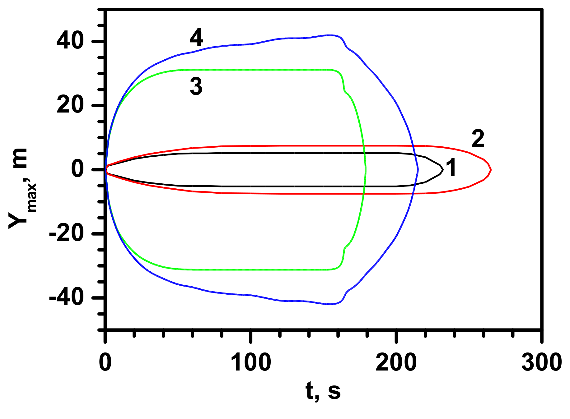
The maximum cloud width, for which values of at least 100% LEL are observed, is between 12 and 18 m, which the Gaussian gas model much better approximates. However, this is clearly more than the predicted value. It could be caused by the effect of crosswinds and increased lateral dispersion.

(e)

Observations made at a short distance from the release location (x ≤ 7 m) indicate that the cloud near the ground surface dissipated in some 15 s, resulting in a more accurate representation of the concentration drop curve provided by the dense gas model for which this time should be approx. 12 s. This is in agreement with simulation results for shorter distances, for which the heavy gas model was more consistent with the results of the field experiment.

(f)

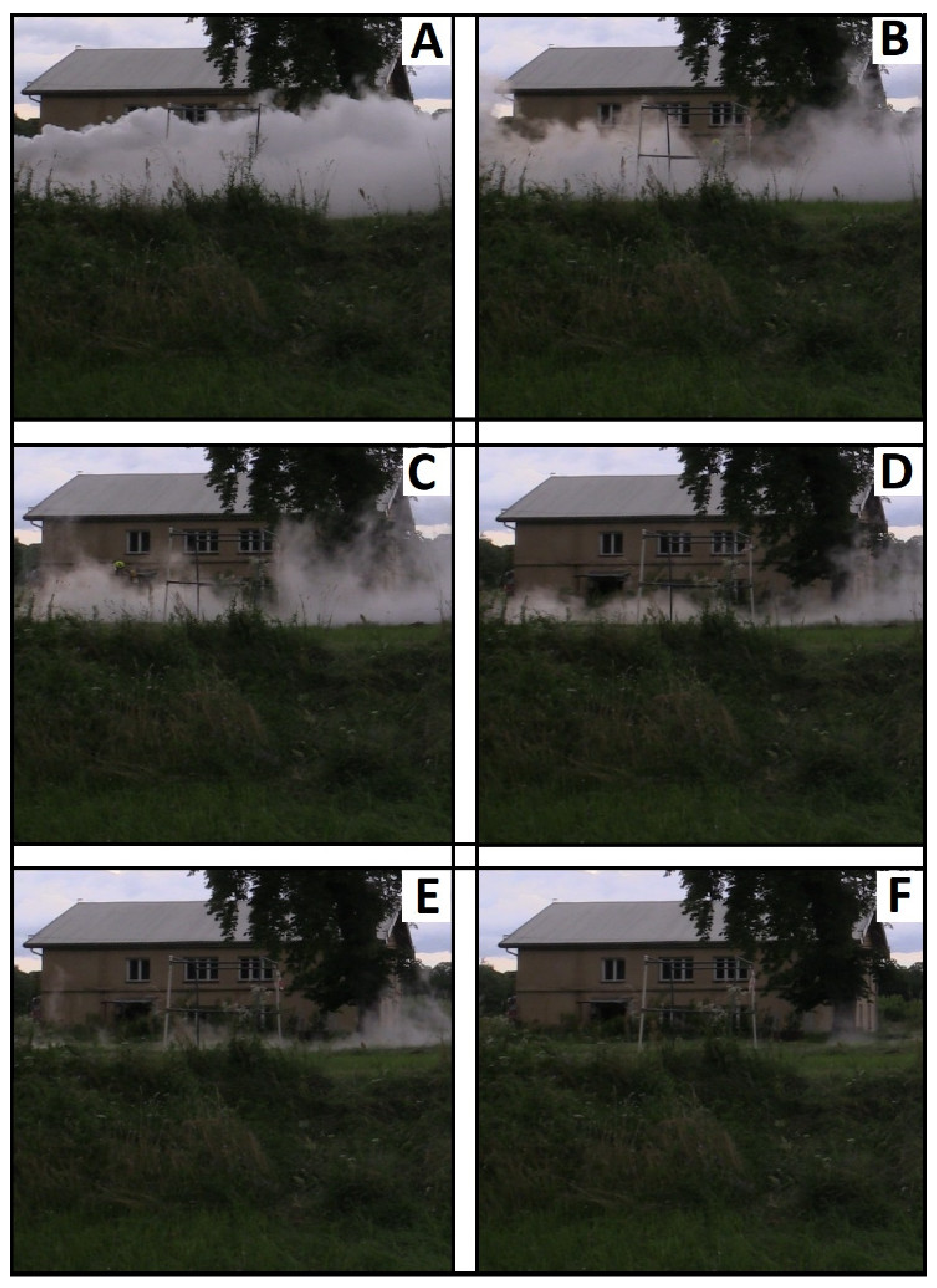
It is shown that concentrations between 71% and 110% LEL are observed at the cloud visibility limit. Nevertheless, the indications of mobile recorders under less stable wind conditions show that the combustible cloud downwind can temporarily move up to 20 m beyond the visible condensation cloud. Such a result means that during rescue operations with uncontrolled release of LNG, special care should be taken, and danger zone must be constantly monitored. Even small wind fluctuations may lead to the cloud displacement.

(g)

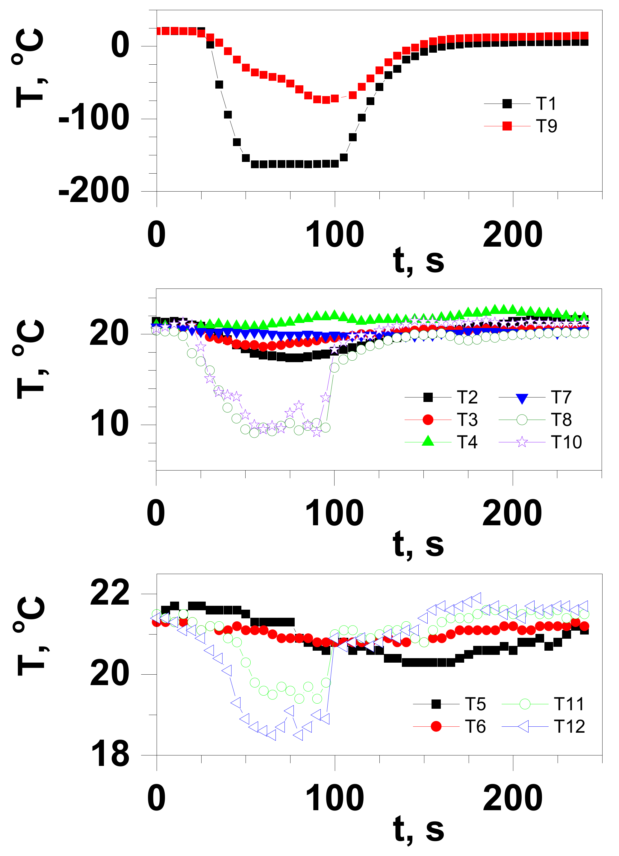
Temperature measurements at a short distance from the cloud release axis (L ≤ 1.25 m) showed only a slight decrease in ambient temperature. However, the maximum value of the temperature drop, in the release axis at the distance where the gas cloud reaches the ground surface, amounts to ∆T_max = 93.3 °C. This indicates that the cloud of the released LNG has almost already completed phase transition at the moment of reaching ground level due to the turbulent outflow of the pressurised gas and the average density of the cloud is lower than the density of the surrounding air. So rapid heating of the cloud explains the preference of passive gas transport at the tested release conditions.

(h)

Exposure to LNG vapours causes the risk of cryogenic burns and cryogenic inhalation only at small distances and, at the temperature of LNG vapours of −73 °C, does not result in a greater than 1% risk of reducing the ability to escape for exposed individuals. For rescue operations, this risk is virtually eliminated because of the guidelines for conducting rescue operations in the release zone requiring the rescuer to be equipped with respiratory protective equipment.

Transport accidents quantitatively account for a very large part of rescue interventions. Due to the growing role of LNG, their probability will undoubtedly increase. So far, there have been only few publications on the analysis of transport hazards from LNG accidents. Therefore, this publication has an important contribution to the development of knowledge on the behaviour of LNG vapours. Better prediction of behaviour of clouds of hazardous gases is extremely important from the point of view of the safety of rescue operations, especially given that there are many types of LNGs, with different compositions, available commercially.

References

- International Gas Union. 2020 World LNG Report; International Gas Union: Vevey, Switzerland, 2020. [Google Scholar]
- Brushlinsky, N.N.; Ahrens, M.; Sokolov, S.V.; Wagner, P. World fire statistics. CTIF 2020, 25. [Google Scholar]
- Woodward, J.L.; Pitblado, R.M. LNG Risk Based Safety. Modeling and Consequence Analysis; Wiley&Sons: Hoboken, NJ, USA, 2010. [Google Scholar]
- Eberwein, R.; Rogge, A.; Behrendt, F.; Knaust, C. Dispersion modeling of LNG-vapor on land—A CFD-model evaluation study. J. Loss Prev. Process Ind. 2020, 65, 104116. [Google Scholar] [CrossRef]
- Nazarpoura, F.; Wen, J.; Dembelea, S.; Udechukwua, I.D. LNG vapour cloud dispersion modelling and simulations with Open FOAM. Chem. Ing. Trans. 2016, 48, 967–972. [Google Scholar]
- Blackmore, D.R.; Colenbrander, G.W.; Puttock, J.S. Maplin Sands experiments 1980: Dispersion results from continuous release of refrigerated liquid propane and LNG. In NATO Challenges of Modern Society-Air Pollution Modelling and Its Application, 3rd ed.; Plenum Publishing: New York, NY, USA, 1984; Volume 5, pp. 353–373. [Google Scholar]
- Ermak, D.L.; Chan, S.T.; Morgan, D.L.; Morris, L.K. A comparison of dense gas dispersion model simulations with burro series LNG spill test results. J. Hazard. Mater. 1982, 6, 129–160. [Google Scholar] [CrossRef]
- Ikealumba, W.C.; Wu, H. Modeling of liquefied natural gas release and dispersion: Incorporating a direct computational fluid dynamics simulation method for LNG spill and pool formation. Ind. Eng. Chem. Res. 2016, 55, 1778–1787. [Google Scholar] [CrossRef]
- Hansen, O.R.; Gavelli, F.; Ichard, M.; Davis, S.G. Validation of FLACS against experimental data sets from the model evaluation database for LNG vapor dispersion. J. Loss Prev. Process Ind. 2010, 23, 857–877. [Google Scholar] [CrossRef]
- Ivings, M.J.; Gant, S.E.; Jagger, S.F.; Lea, C.J.; Stewart, J.R.; Webber, D.M. Evaluating Vapour Dispersion Models for Safety Analysis of LNG Facilities; Final report; HSL: Buxton, UK, 2016. [Google Scholar]
- Sklavounos, S.; Rigas, F. Fuel gas dispersion under cryogenic release conditions. J. Energy Fuels 2005, 19, 2535–2544. [Google Scholar] [CrossRef]
- Luketa-Hanlin, A. A review of large-scale LNG spills: Experiments and modeling. J. Hazard. Mater. 2005, 132, 119–140. [Google Scholar] [CrossRef] [PubMed]
- Pontiggia, M.; Derudi, M.; Busini, V.; Rota, R. Hazardous gas dispersion: A CFD model accounting for atmospheric stability classes. J. Hazard. Mater. 2009, 171, 739–747. [Google Scholar] [CrossRef] [PubMed]
- Shih, T.H.; Liou, W.W.; Shabbir, A.; Yang, Z.; Zhu, J. A new—Eddy-viscosity model for high Reynolds number turbulent flows—Model development and validation. Comput. Fluid 1995, 24, 227–238. [Google Scholar] [CrossRef]
- Zapert, J.G.; Lordengan, R.J.; Thistle, H. Evaluation of Dense Gas Simulation Models; EPA: Research Triangle Park, NC, USA, 1991.
- Guo, D.; Zhao, P.; Wang, R.; Yao, R.; Hub, J. Numerical simulation studies of the effect of atmospheric stratification on the dispersion of LNG vapor released from the top of a storage tank. J. Loss. Prev. Process Ind. 2019, 61, 275–286. [Google Scholar] [CrossRef]
- Luo, T.; Yu, C.h.; Liu, R.; Li, M.; Zhang, J.; Qu, S. Numerical simulation of LNG release and dispersion using a multiphase CFD model. J. Loss. Prev. Process Ind. 2018, 56, 316–327. [Google Scholar] [CrossRef]
- Siuta, D.; Markowski, A.S.; Mannan, M.S. Uncertainty techniques in liquefied natural gas (LNG) dispersion calculations. J. Loss Prev. Process Ind. 2013, 26, 418–426. [Google Scholar] [CrossRef]
- Koopman, R.P.; Caderwall, R.D.; Ermak, D.L.; Goldwire, H.C., Jr.; Hogan, W.J.; McClure, J.W.; McCrae, T.G.; Morgan, D.L.; Rodean, H.C.; Shinn, J.H. Analysis of Burro series 40m3 LNG spill experiments. J. Hazard. Mater. 1982, 6, 43–83. [Google Scholar] [CrossRef]
- Ermak, D.L.; Chapman, R.; Goldwire, H.C., Jr.; Gouveia, F.J.; Rodean, H.C. Heavy Gas Dispersion Test Summary Report; Report No. UCRL-21210; Lawrence Livermore National Laboratory: Livermore, CA, USA, 1988. [Google Scholar]
- Jones, R.; Lehr, W.; Simecek-Beatty, D.; Reynolds, R.M. ALOHA (Areal Locations of Hazardous Atmospheres) 5.4.4: Technical Documentation; U.S. Dept. of Commerce: Washington, DC, USA; NOAA Emergency Response Division: Seattle, WA, USA, 2013.
- Planas-Cuchi, E.; Gasull, N.; Ventosa, A.; Casal, J. Explosion of a road tanker containing liquefied natural gas. J. Loss Prev. Process Ind. 2004, 17, 315–321. [Google Scholar] [CrossRef]
- Bonilla Martinez, J.M.; Belmonte Perez, J.; Marin Ayala, J.A. Analysis of the explosion of a liquefied-natural-gas road-tanker. Segur. Medio Ambiente 2011, 32, N127. [Google Scholar]
- Laciak, M.; Oliinyk, A.; Sikora, A.P.; Wlodek, T. Effect of composition variability of liquified natural gas propiertiesin term of storage process stability. Przem. Chem. 2018, 97, 267–271. [Google Scholar]
- Bakkum, E.A.; Duijm, N.J. Vapour cloud dispersion. In Methods for the Calculation of Physical Effects—Due to Releases of Hazardous Materials (Liquisds and Gases), Yellow Book (Cpr14e), 3rd ed.; van der Bosch, C.J.H., Weterings, R.A.P.M., Eds.; Gevaarlijke Stoffen: The Hague, The Netherlands, 2005. [Google Scholar]
- Hanna, S.R.; Chang, J.C.; Strimaitis, D.G. Hazardous gas model evaluation with field observations. Atmos. Environ. 1993, 27, 2265–2285. [Google Scholar] [CrossRef]
- Hanna, S.R.; Strimaitis, D.G.; Chang, J.C. Hazard Responce Modeling Uncertainty (a Quantitative Method). Evaluation of Commonly Used Hazardous Gas Dispersionmodels; Final report to the engineering and services laboratory; Air Force Engineering and Services Center: Tyndall Air Force Base, FL, USA, 1991; Volume 2. [Google Scholar]
- Sun, B.; Wong, J.; Wadnerkar, D.; Utikar, R.P.; Pareek, V.K.; Guo, K. Multiphase simulation of LNG vapour dispersion with effect of fog formation. Appl. Therm. Eng. 2020, 166, 114671. [Google Scholar] [CrossRef]
- Shaikh, I.; Porter, L. Incorporating asphyxiation and cryogenic hazards into risk analysis. In Proceedings of the 11th Annual Mary Kay O’Connor Process Safety Center Symposium, College Station, TX, USA, 28–29 October 2008. [Google Scholar]