Abstract
Recent episodes of natural disasters have challenged the resilience of power grids. Adequate distribution grid planning that properly captures the risk aversion of the utility system planner is a key factor to increase the flexibility of distribution networks to circumvent these events. In this paper, we propose a methodology to determine the optimal portfolio of investments in lines and storage devices in order to minimize a convex combination between expected value and CVaR of operational costs, including energy not served, while taking into account the multistage nature of the energy storage management within this context. While the expected value of energy not served has been traditionally employed to tackle routine failures, we also minimize the CVaR of energy not served to address high-impact, low-probability (HILP) events. We illustrate the performance of the proposed methodology with a 54-Bus system test case.
1. Introduction
Traditional distribution grid planning is primarily focused on reliability metrics [1] and comprises the application of simulation-based probabilistic evaluation techniques [2], which were later updated to include emerging challenges of power distribution reliability, such as the presence of distributed energy resources (DERs) [3]. More recently, these reliability targets started to be added in the context of expansion and planning of distribution grids, a class of methods aiming at optimizing the portfolio of network infrastructure investments, including substation/circuit upgrade and reinforcement [4,5].
However, recent episodes of natural disasters such as floods, windstorms, or earthquakes have caused billions of dollars of irreparable damage in grid assets and long-term interruption of service [6,7], raising governments awareness regarding resilience of energy infrastructures [8] to face these high-impact, low-probability (HILP) events. From a power grid perspective, these events are different from normal routine failures captured by reliability indices and they require specific resilience metrics, evaluation techniques as well as new approaches to include them into the economic expansion and planning problem. Similarly to reliability evaluation, simulation techniques have been proposed in the context of resilience to assess the power grid’s ability to withstand, mitigate, and recover from extreme events. In general, these techniques rely on two types of approaches: (i) methods that do not require a detailed model of the extreme events, such as complex networks (CN) methodologies that assess resilience based on network topological characteristics [9,10]; (ii) Monte Carlo methods based on probabilistic models of the events combined with fragility curves to simulate network failures and their HILP consequences [11,12]. Instead of looking at the routine aspects (i.e., expected value) of the outage impacts, these resilience probabilistic models are often focused on the tails of outage distributions, describing resilience as risk metric, such as Value at Risk (VaR) or Conditional Value at Risk (CVaR), associated with the loss of load [13].
According to [14], there are three main stages when dealing with critical disruptive events that challenge the resilience of power grids: (a) the first stage is the resilience investment, done years ahead of the events; (b) the second and third stages are corrective actions and restoration, respectively, which take place during and after the event materializes. In this paper, we present a methodology to determine investments in new lines and storage devices in order to address the first stage in a way that facilitates corrective actions to minimize the energy not served when a critical event takes place.
Stochastic optimization is a powerful framework to solve investment problems under uncertainty and has been employed in relevant works that address resilience investments in power grids. At the transmission system level, a two-stage stochastic MINLP model was presented in [15] to find investment strategies to improve resilience, considering a range of earthquake events. In distribution grids, a storage sitting and sizing model to maximize resilience against seismic hazards is presented in [16]. The method takes the earthquake fragility curves as an input and solves the storage planning problem through a combination of heuristics (to select candidate nodes) and linear programming. An extension to mobile storage investments, using stochastic resilience optimization solved via progressive hedging (PH), is proposed in [17]. Additional network investments are considered in the context of earthquake impact mitigation through a two-stage optimization via simulation method [18]. An analogous two-stage approach is presented in [19], considering circuit hardening, automatic switches and DER investments to mitigate extreme weather events.
A number of works have recently addressed the distribution grid planning problem as discussed in [20]. Some pertinent examples are [21,22,23,24,25,26,27,28,29,30] to mention a few. In [21], a stochastic optimization-based methodology is presented to address the distribution system planning by selecting investments in batteries, feeders, and substations while considering uncertainty in demand and electricity prices as well as the impact of battery degradation. In [22], a trilevel model is proposed to identify line hardening solutions to protect the distribution grid against intentional or unintentional attacks. In [23], a methodology is developed to plan distribution grids while considering the flexibility provided by thermal building systems to reduce peak demands and consequently the grid capacity requirements. In [24], an algorithm that combines particle swarm optimization and tabu search is presented to plan the expansion of large electric distribution networks. In [25], the authors propose to plan the distribution system expansion while taking electric vehicles and uncertainty in renewable energy sources into account. In [26], the authors present a methodology to expand the distribution system while considering three different players, namely the distribution company (DISCO), the private investor (PI) who owns distributed generation, and the demand response provider (DRP). On one hand, PI and DRP are risk-averse and therefore seek to maximize the CVaR of their profits due to the existing uncertainty in renewable generation and availability of demand response. On the other hand, the DISCO aims to upgrade the system (via line reinforcement) to minimize cost and increase reliability in a risk-neutral fashion by minimizing expected energy not served due to failures of lines. In [27], a methodology is proposed to select investments in dispatchable units, DER units, and line reinforcement while considering uncertainty in load and DERs production and adequacy to this uncertainty without taking into account failure of system elements. In [28], the distribution planning problem is approached from a game-theoretical perspective. In [29], a bilevel mixed-integer programming model is proposed to determine the distribution system expansion planning considering the contribution of electric vehicles (EVs) in public parking lots. The first level sets grid investment decisions in circuits and substations, while the second level optimizes the EV charging strategies to achieve maximum parking lot remuneration from grid services. Although the framework presented in [29] is interesting, the proposed solution approach does not guarantee optimality as the solution method is based on an immune genetic algorithm. In [30], the authors propose a two-stage robust optimization model to select investments in line hardening and distributed generation. Despite its resilience oriented objective, the work in [30] is specific for hurricanes and does not cover other extreme events. The relevance of the aforementioned papers notwithstanding, to the best of our knowledge, there is still no work in the literature that models and solves to optimality the decision making process of a risk-averse distribution system planner that needs to select investments in lines and storage devices to minimize a convex combination between expected value and CVaR of costs while taking the multistage nature of storage devices operation into account. In this paper, we aim to bridge this gap.
In this paper, we present a stochastic optimization model for expansion planning of distribution grids considering both reliability and resilience criteria, thus adding to the existing approaches that either consider reliability [4,5] or resilience [15,16,17,18,19] in this problem. We propose a static expansion planning model (i.e., investment decision can be taken only once) where the operation of the system in the short term is modeled in a multistage fashion. We consider different distribution grid investments to minimize the expected value and the CVaR associated with outages caused by routine failures and HILP events. Differently from [15,16,17,18,19], our model takes into account investment in storage devices and the corresponding multistage nature of their operation under uncertainty. More specifically, we formulate a stochastic optimization problem as a mixed integer linear program (MILP) where, once investment takes place, the operation of the system is modeled as a multistage problem. In order to circumvent tractability issues associated with the size of the problem, we develop a solution methodology based on nested Benders decomposition. While this decomposition approach is traditionally employed to minimize the expected value metric [31,32], our tailored multistage temporal decomposition is also capable to minimize the CVaR metric, adding risk aversion to decision making. The result is an innovative investment planning approach where the “reliability vs. resilience” preferences of the planner are explicitly provided as an input of the problem. The specific contributions of this paper are twofold:
- 1.
- A stochastic investment and planning model for distribution grids with risk-based explicit metrics that allow utilities and network planners to explore the trade-offs between reliability and resilience when selecting the best portfolio of conductors and DER investments. This model is able to capture the system operation, in particular the multistage aspects of time-coupling constraints related with energy storage management.
- 2.
- A tailored novel temporal decomposition framework that renders a tractable and effective solution approach for the model and accommodates the minimization of expected value and CVaR of the operational costs, including energy not served.
The remainder of this paper is laid out as follows. In Section 2, we present the mathematical formulation to model. We describe the proposed solution methodology in Section 3. In Section 4, a case study with a 54-bus test system illustrates the proposed methodology. In Section 4, the proposed methodology is illustrated through a case study based on a 54-bus test system. Finally, we draw the conclusions in Section 5.
2. Mathematical Formulation: Incorporating Risk Aversion into Distribution Grid Planning
The proposed model aims at determining the optimal investments in line branches and/or storage devices to improve the system performance in terms of reliability. As in [4,5], we formulate this planning problem as a MILP. Nevertheless, unlike [4,5], we also consider the impact of HILP events in our formulation and the installation and operation of storage devices. Our proposed formulation is a static expansion planning problem (i.e., investment decision can be taken only once) with a multistage representation of the short-term system operation. That being said, once an investment decision is made (for a target year as customary in static expansion planning models [33]), the system is operated for a set of typical days that represent a certain horizon (e.g., one year). The stages basically represent short-term operation within each typical day, i.e., each stage comprises some hours of operation. In this manner, we can model the multistage nature of the management of the states of charge of the storage devices.
We illustrate in Figure 1 our modeling framework when considering two typical days with three stages each (an illustrative example of this modeling framework is also provided in the link where we provide input data for the case study). In this framework, investment decisions are taken only in the first stage. As can be seen, each day has a given load profile and is constituted of a scenario tree, composed by different stages . Each stage contains a set of scenario tree nodes m, with a set of hours . The storage operation is modeled throughout each day d and its respective scenario tree, in which the node m comprises a given state of grid (which is assumed to be a given parameter) that represents the current network configuration with each element being equal to 1 if line l is available and switched on for scenario tree node m, hour, t and day d or 0 if the line is either out-of-service (due to failure) or switched off (due to radiality constraints). The transition probabilities indicate how likely it is to reach a scenario tree node m that comprises one or more failures. Naturally, scenarios tree nodes associated with HILP events and the failure of more than one line have a much lower transition probability. If the planner is interested is just minimizing the expected value of operational costs when determining the investment decisions, scenarios tree nodes comprising HILP events will have little or no impact in the final expansion plan. As a result, the first-stage investment decision will not include lines that need to be activated according to due to the failure of other lines during a HILP event. In addition, this investment decision will not comprise extra necessary installation of storage devices either. Therefore, as one of the main contributions of this paper, we provide a methodology general enough to minimize the convex combination between expected value and CVaR of the operational costs, including energy not served. In this manner, we can properly capture the effect of the HILP events while expanding the system in a risk-averse fashion.
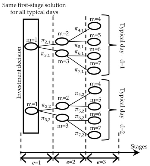
Figure 1.
Modeling framework.
In the next subsections, we describe the proposed MILP formulation that mathematically represents our model.
2.1. Costs and Risk-Averse Modeling
The costs associated with investments and operation are modeled as follows.
The objective function (1) to be minimized comprises a weighted sum of the overall costs associated with each day , represented in a recursive manner. For instance, considering an annual operation, parameter corresponds to the number of days in the year that can be represented by day d in terms of load profile and probability of line outages.
Constraints (2)–(6) describe one of the main modeling features that we aim to address in this paper. Here, we combine risk-neutral (expected value) and risk-averse (CVaR) metrics in order to consider both reliability (associated with routine events) and resilience (associated with HILP events) as targets. For instance, in (3), a risk-neutral planner would set and minimize only the expected value of the costs, therefore neglecting HILP events as they are present scenario tree nodes with small transition probabilities . A non-risk-neutral planner, on the other hand, would set a higher than zero in order to determine a plan that also minimizes the CVaR of the costs and therefore captures the impact of HILP events. Thus, the convex combination in (3) allows for the planner to express their level of risk aversion. The higher this risk aversion, the higher the planner will set the value of so as to put more weight on the CVaR metric in the objective function. In this recursive framework, the scenario tree nodes that belong to the last stage of each are the base case and their overall cost (2) is simply equal to the cost of the current scenario tree node, . In their turn, the remaining nodes (not in the last stage) comprise an additional cost (3), formed by a convex combination between the expected value and the CVaR of the cost of the descendent nodes (i.e., the kid nodes), contained in set . Constraints (4)–(6) complement the modeling of the CVaR of the cost of the next stage for each scenario tree node m and day d.
Constraints (7) represent the cost of investment and operations associated with each scenario tree node m. The investment cost comprises new lines and storage devices while the operation costs include power injections in the substation, transformer and line losses, as well as energy not served. As explained in the next subsections, investment can only be made at the first stage, so for most of the scenario tree nodes m, no investment decision is considered. The transformer and line losses penalized in (7) are represented through piecewise linear approximations via expressions (8)–(12).
2.2. Investment in Lines
The investment in lines is mathematically described as follows.
Constraints (13) impose the binary nature to variables and constraints (14) do not allow investment at scenario tree nodes that do not belong to the first stage. Constraints (15) enforce the same investments in lines to be made for all considered days . Expressions (16)–(18) model the transition between stages of the decisions on line investments. The index in (17) signifies the parent node of scenario node m. In Figure 1, for example, for , we have as scenario node 1 is the parent of scenario node 2. Within this context, expression (17) carries information from the parent scenario node to the current scenario node m. In this stagewise communication setting, each scenario node only receives information from the immediate predecessor node (the parent node).
2.3. Investment in Storage Devices
The investment in storage devices is expressed as follows.
Constraints (19) describe as binary variables. Constraints (20) enforce no binary investments to be made in storage devices at scenario tree nodes that do not belong to the first stage. Constraints (21) impose the same binary investments in storage devices to be made for all considered days . Expressions (22)–(24) model the transition between stages of the decisions on binary investments in storage devices. Analogously, constraints (25)–(30) model continuous investments in storage devices, where is the maximum investment in storage device h.
2.4. Operation of the Grid
The operation of the network is modeled as follows.
Constraints (31)–(38) present a linear grid operation model proposed in [34] and used in other works such as [4]. Constraints (31) and (32) limit the substation injection and nodal voltages, whereas (33) and (34) impose flow limits to existing and candidate lines. According to (33) and (34), existing and candidate lines can be utilized if they are part of the current configuration or state of the grid, i.e., their respective parameters are equal to 1. Otherwise, if for a certain line, such a line is open. Expressions (35) and (36) represent the nodal power balance of buses with and without a substation. Power flows are described in a linear fashion by constraints (37) and (38).
2.5. Operation of Storage Devices
The operation of storage devices is modeled as follows.
Constraints (39) and (40) impose, for existing and candidate storage devices, the value of state of charge for the last period of the scenario tree nodes that belong to the last stage. Constraints (41)–(47) model the transition of the state of charge of the existing and candidate storage devices throughout the stages of the scenario tree of each considered day . Constraints (41)–(47) impose the limits of charging/discharging and state of charge for existing and candidate storage devices.
3. Solution Methodology: Solving the Risk-Averse Multistage Problem
Model (1)–(53) is a multistage formulation, where at each scenario tree node the objective is to minimize the convex combination of expected value and CVaR of the cost of the nodes of the next stage. This formulation can easily become intractable even for medium-sized systems and a reasonable number of scenarios. Hence, in this section we propose a multistage decomposition that circumvents the tractability issues associated with the proposed model.
To start the solution methodology involves the iterative solution of Algorithm 1 and 2, which will be described in this Section. In order to develop this solution methodology, first, we rewrite (1)–(53) as:
where expressions (54) and (55) replicate (1)–(6), whereas constraints (56) are equivalent to (7). Constraints (57)–(60) represent (13)–(15), (19)–(21) and (25)–(27). Constraints (61) and (62) correspond to (8)–(12), (31)–(38) and (46)–(53). Finally, constraints (63)–(65) are associated with (16)–(18), (22)–(24), (28)–(30) and (39)–(45), which contain the inter-temporal coupling constraints.
A reasonable size system combined with plausible number of stages and scenario tree nodes can render problem (54)–(65) easily intractable due to the high number of constraints involved. In order to withstand this tractability problem, here, we propose a nested-Benders-type algorithm. To do so, we decompose the problem (54)–(65) into a master problem for the first stage and several subproblems, each one corresponding to a remaining stage. The master problem is formulated as follows:
Essentially, the master problem describes the decision making process of the first stage of (54)–(65), where decisions on investments in lines and storage devices are determined. In addition, the master problem approximates the objective function of the scenario tree nodes that belong to the second stage by means of expression (78). The subproblems are formulated as follows.
| Algorithm 1: Compute . |
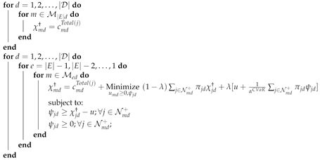 |
The subproblems in the form of (79)–(89) represent the operation in each of the remaining stages, where the variables in parentheses correspond to the dual variables related to the transition constraints. Analogously, the objective functions of the scenario tree nodes that emanate from the current one are approximated via (89).
| Algorithm 2: Solution algorith. |
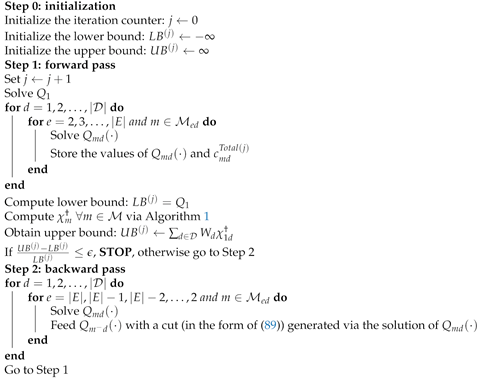 |
Thus, the solution algorithm relies on an iterative process between master and subproblems, comprising forward and backward passes as shown in Algorithm 2. In the forward pass, first, the master problem (66)–(78) is solved and then, for each day d and each stage e (going from the first to the last stage), the subproblems (79)–(89) are solved. At this step, each scenario tree node receives information from its parent scenario tree node in the form of , and , which propagate decisions on investments throughout the scenario tree and notify the state of charge of the batteries. Once the forward pass is completed, a lower bound for the current iteration is set equal to the current value (see (66)). On the other hand, an upper bound is calculated by making use of the values of obtained during the forward pass. First, values of are computed via Algorithm 1. Then, the upper bound is set equal to . In case the convergence criterion is not met, the backward pass is executed. In this step, again, (79)–(89) is solved for each day d and each stage e (going from the last to the second stage) in order to provide relevant information that is used to build the approximations (78) and (89).
4. Case Study
The performance of the proposed methodology is analyzed and illustrated with a 54-bus distribution system (depicted in Figure 2) based on [4]. We consider 50 load nodes, 4 substations, 50 existing lines, 22 candidate lines, and 4 candidate nodes to receive storage devices (up to 400 units of 6kWh at each node). The proposed methodology has been implemented on a Linux server with two Intel® Xeon® E5-2680 processors @ 2.40GHz and 64 GB of RAM, using Julia 1.1, JuMP and solved via CPLEX 12.9.
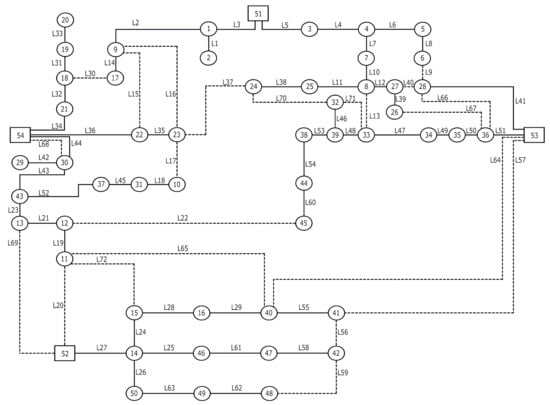
Figure 2.
54-bus system—Existing line segments are the solid lines and candidate lines are the dashed lines. Buses 2, 19, 20, and 26 are candidates to receive investment in storage.
In this case study, regarding routine failures, we consider that all (existing and candidates) lines have a rate of failure of 0.4 times per year (i.e., on average they fail once every 2.5 years), regardless of their length. In addition, we consider five critical failures with a rate of 0.01 times per year to mimic the nature of HILP events. Two of these critical failures involve outages of two lines simultaneously, whereas the other three comprise the outage of three lines simultaneously.
The routine and critical failures and their respective rates are used to build scenario trees that represent typical days of operation. More specifically, at each stage, the scenario tree node without any current failure has a probability to transition into a scenario tree node with a single outage in any line of the system according to its failure rate. In addition, such scenario tree node has a probability of transitioning into a scenario tree node with a critical failure involving more than one line according to the failure rate associated with this critical failure. We assume these failures rates are provided by the system operator. Nevertheless, it is important to emphasize that we use these scenarios as an input for the proposed methodology. Developing a scenario generation technique is out of the scope of this paper.
We take into account four typical days whose demand profiles are depicted in Figure 3. As the study comprises one year of operation, we consider that typical day one repeats 15 times, typical day two repeats 110 times, typical day three repeats 163 times, and typical day four repeats 77 times, adding up to 365 days. As aforementioned, each typical day is described via a scenario tree of six stages, where each stage consists of four hours of operation.
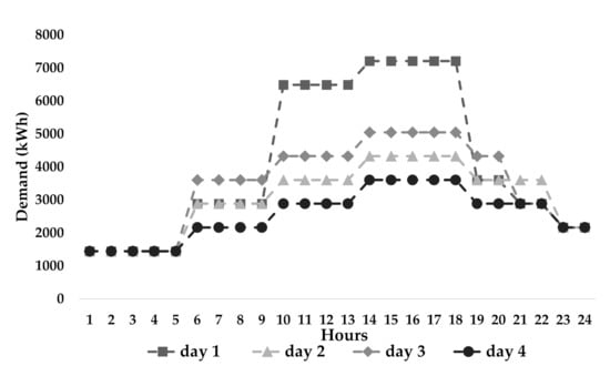
Figure 3.
Demand profiles.
4.1. Investment Results
To illustrate the methodology, we compare three risk aversion policies and their impact on the expansion plan. In the first one, we set in expression (3). This choice of indicates a reliability-oriented expansion plan focused on minimizing the expected costs associated with investment and operation of the system. In the second plan, we set , which corresponds to a choice for a reliability and resilience oriented expansion plan. According to (3), this plan minimizes both expected value and CVaR of the overall costs. In the third plan, we set in order to obtain an expansion plan that minimizes the CVaR of the overall costs. Table 1 compares these three plans. As expected, when the CVaR of the total costs is taken into account, more lines are needed. Notably, the number of storage units is particularly influenced by an increase in the risk aversion parameter.

Table 1.
Obtained expansion plans.
4.2. Discussion: Out-of-Sample Analysis
To evaluate the performance of the three aforementioned obtained expansion plans, we have performed an out-of-sample analysis, generating 2000 annual scenarios. In each scenario, for each four-hour interval of the year, we generated a Bernoulli trial for line states (1 in service; 0 failure) with probabilities according to the rate of routine and critical failures previously mentioned. Then, the performances of the three plans resulting from the different risk aversion policies were simulated and compared with a base case without investments.
At first glance, this comparison can be seen in Figure 4, which depicts the inverse probability distribution of the annual energy not served. As illustrated in this figure, the base case (no investments) incurs in much higher probability to result in non-negligible values of annual energy not served in comparison to the considered expansion plans.
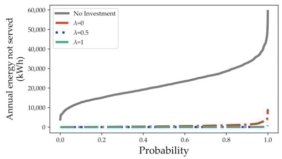
Figure 4.
Out-of-sample analysis—Inverse probability distribution of the annual energy not served.
In the next subsections, we present comparisons between the expansion plans and the base case in terms of reliability and risk aversion metrics.
4.2.1. Reliability
In Table 2 and Figure 5, we present the results of this analysis in terms of reliability. Table 2 shows three metrics, namely, average of annual energy not served (also known as expected energy not served), SAIFI (system average interruption frequency index), and SAIDI (system average interruption duration index). In addition, Figure 5 displays the number of hours (in logarithmic scale) for each non-negligible level of average hourly energy not served. It is clear that the system is more reliable as investments are made and, therefore, the energy not served decreases with the increase of the parameter . Moreover, by analyzing solely Figure 5, one can conclude that if the average energy not served (representing reliability) is the only metric of interest, the expansion plan considering and even the system without any investment have an acceptable performance, as the maximum average energy not served for the base case is less than 0.2% of the system demand.
Table 2.
Out-of-sample analysis—Reliability metrics: Average annual energy not served, SAIFI, and SAIDI.
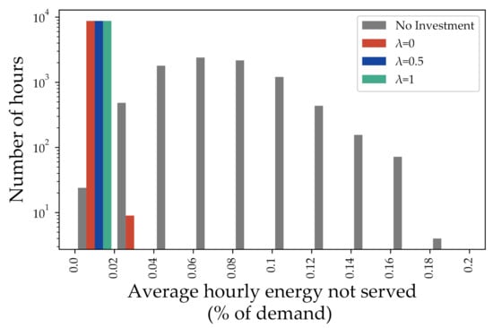
Figure 5.
Out-of-sample analysis—Average hourly annual energy not served.
4.2.2. Risk Aversion
In order to compute risk-aversion metrics for each expansion plan and the base case, first, we obtained the annual energy not served for each of the simulated annual scenarios of operation. Then, with the 2000 values of annual energy not served in hand, we calculated the CVaR, the CVaR and the worst case of annual energy not served, which are shown in Table 3. Clearly, the system is less exposed to the risk of incurring in annual energy not served as investments take place and the value of the risk aversion parameter is increased.
Table 3.
Out-of-sample analysis—Risk aversion metrics (CVaR, CVaR and worst case) of annual energy not served.
In addition, for each hour of the year, we have computed the CVaR and the worst-case energy not served across the 2000 scenarios. These results are reported in Figure 6 and Figure 7. As can be noticed, unlike Figure 5, Figure 6 and Figure 7 explicitly illustrate the importance of taking risk aversion into consideration to increase the resilience of the system by decreasing its levels of energy not served during HILP events. More specifically, it can be noticed in Figure 6 and Figure 7 that the base case (no invesment) and the risk-neutral (and solely reliability-oriented) expansion plan obtained with may incur in unacceptable levels of risk, reaching more than 20% of energy not served in the worst case (and even more than 36% for the base case). On the other hand, the system is much less exposed to risk when expansion plans (obtained via the proposed methodology) for and take place.
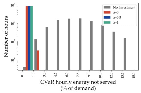
Figure 6.
Out-of-sample analysis—CVaR of hourly energy not served.
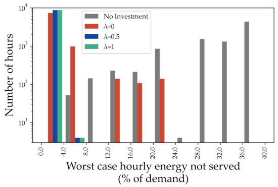
Figure 7.
Out-of-sample analysis—Worst case of annual energy not served.
4.3. Discussion: Risk-Aversion Parameter
In our proposed approach, the system planner is provided with opportunity to define their level of risk aversion. There are different degrees of risk aversion. In finance, for example, different investors may have different risk aversion profiles depending on how much risk they are willing to take to achieve some level of investment return. In our case, the more risk averse a system planner is, the bigger the amount of investment they will be willing to make to avoid the realization of scenarios associated with high loss of load. Within our framework, the parameter represents the risk aversion of the system planner. The higher the , the more risk averse the planner is because the CVaR will have more weight on the objective function.
Providing general guidelines to set the value of the risk aversion parameter is not a focus of this paper, as we assume the system planner will have more information to determine the value of this parameter. However, here, we suggest three steps that can be followed as a basic procedure to understand which values of can be suitable for a particular planner. First, the planner should observe the investment costs associated with each considered value of . In our case study, we show these costs in Table 1. By comparing these costs with their investment budget, the system planner can immediately identify which values of (and their corresponding investment plans) are actually achievable. Second, the planners should consider the values of reliability indexes associated with each . In our case study, we show these metrics in Table 2. Every utility company has predefined targets of average annual energy not served—SAIFI and SAIDI, for example. In this case, the values of that correspond to investment plans that comply with targets of reliability are naturally good candidates. As we can see in Section 4.2.1, the investment plan associated with already significantly improves reliability metrics. Third, the planner needs to observe the risk aversion metrics, which we show in Table 3 for our case study. Here, the planner would also need to define which values of CVaR and worst-case annual energy not served are acceptable in order to choose the appropriate value of and its corresponding investment plan. Once the aforementioned three steps are taken, the planner will have investment plans associated with different values of that comply with reliability and risk-aversion metrics. With these investment plans in hand, a choice for the least-cost one will be natural.
4.4. Discussion: Imposing Investment Budget Constraint
In this section, we assess the behavior of the proposed methodology under an investment budget constraint. To do so, we have included an extra constraint that imposes that the investment to expand the grid cannot exceed $300,000.00. The results in terms of investments are shown in Table 4.
Table 4.
Obtained expansion plans under investment budget constraint.
As can be seen by comparing Table 1 and Table 4, the investment for does not change as the optimal investment plan for this case was already cheaper than the imposed budget limit. For and , however, there is a significant change in the investment plan due to the restrictive investment constraint. More specifically, it is interesting to see that the methodology invests in more batteries instead of including another line segment for and when investment is constrained. From to , it is also interesting to notice that location of the new storage units change. This result indicates that storage devices are preferable than new line segments when investment is limited for the 54-bus system under consideration.
5. Conclusions
In this paper, we proposed a methodology to address expansion planning of distribution networks in a risk-averse manner. In this methodology, we provide the system planner with the flexibility to balance the trade-off between focusing on expected value or CVaR of energy not served costs, therefore enabling an explicit form of controlling risk and adjusting the grid planing to cope with routine and extreme event failures. Within this context, our proposed methodology determines the optimal portfolio of lines and storage devices to be installed in the grid so as to increase its reliability and resilience. In addition, our methodology properly models the multistage nature of the energy management decisions regarding reliability/resilience utilization of storage devices. Our numerical results demonstrate that it is imperative to consider risk aversion while expanding distribution grids in order to increase the resilience of distribution systems. In our proposed modeling, if the system transitions to a scenario node where a certain line segment has failed at a given stage, for the following stages (i.e., until the end of the typical day), the system will either transition to scenario node with the same failure or with to a node with an additional failure. In this case, investment made will have the potential to prevent or alleviate the loss of load associated with the failures. As a potential future work, it would be also interesting to model the repair time within our framework.
Author Contributions
Conceptualization, A.M. and M.H.; methodology, A.M.; software, A.M. and A.V.; validation, A.M., A.V. and M.H.; formal analysis, A.M.; data curation, A.M.; writing—original draft preparation, A.M.; writing—review and editing, A.M. and M.H.; visualization, A.M. and A.V.; project administration, A.M. and M.H.; funding acquisition, M.H. All authors have read and agreed to the published version of the manuscript.
Funding
This research was supported by the US Department of Energy under Contract No. DE-AC02-05CH11231.
Data Availability Statement
For replicability purposes, input data used in this paper can be downloaded from (13 December 2021) https://drive.google.com/drive/folders/1LmgufcIdIDbMgKbh0mY6wIK6abl914et?usp=sharing.
Conflicts of Interest
The authors declare no conflict of interest.
Nomenclature
| Sets | |
| Set of typical days. | |
| Set of indices of all buses (including substations and nonsubstations). | |
| Set of indices of buses that are substations. | |
| E | Set of stages. |
| H | Set of indices of all storage devices (including existing and candidates). |
| Set of indices of candidate storage devices | |
| Set of indices of all lines (including existing and candidates). | |
| Set of indices of candidate lines. | |
| Set of indices of existing lines. | |
| Set of indices of scenario tree nodes. | |
| Set of indices of scenario tree nodes that belong to day d. | |
| Set of indices of scenario tree nodes that are “kids” of scenario tree node m. | |
| Set of time periods of each scenario tree node. | |
| Indices | |
| d | Index of typical days. |
| e | Index of stages. |
| Index of the stage to which scenario tree node m belongs. | |
| h | Index of storage devices. |
| l | Index of lines. |
| n | Index of buses. |
| m | Index of scenario tree nodes. |
| Index of the scenario tree node that is the parent of scenario tree node m. | |
| t | Index of time periods. |
| Parameters | |
| CVaR parameter. | |
| Maximum amount of flow in line l associated with jth piecewise linear function used to linearize losses. | |
| Maximum amount of substation injection in bus n associated with jth piecewise linear function used to linearize losses. | |
| Slope of jth piecewise linear function used to linearize losses multiplied by respective impedance . | |
| Slope of jth piecewise linear function used to linearize losses multiplied by respective impedance . | |
| Risk aversion user-defined parameter (between 0 and 1). | |
| Probability of transition to scenario tree node m in day d. | |
| Fixed investment cost of candidate line l. | |
| Cost of imbalance. | |
| Cost of losses. | |
| Fixed investment cost of candidate storage device h. | |
| Variable investment cost of candidate storage device h. | |
| Injection cost in substation n at scenario tree node m and day d. | |
| Maximum capacity of existing line l. | |
| Limit of injection in substation n. | |
| M | Sufficiently large number. |
| Number of piecewise linear functions used to linearize losses. | |
| Maximum charging of storage device h per stage. | |
| Maximum discharging of storage device h per stage. | |
| Power factor. | |
| Length of line l. | |
| Number of time periods to fully charge storage devices. | |
| Initial and final stored energy in storage device h. | |
| Minimum voltage. | |
| Maximum voltage. | |
| Maximum investment in storage device h. | |
| Parameter that determines if line l is available (being equal to 1) or unavailable (being equal to 0). | |
| Impedance of line l. | |
| Decision variables | |
| Amount of flow in line l associated with jth piecewise linear function used to linearize losses. | |
| Amount of substation injection in bus n associated with jth piecewise linear function used to linearize losses. | |
| Positive imbalance in bus n. | |
| Negative imbalance in bus n. | |
| CVaR auxiliary variable. | |
| Total cost of scenario tree node m. | |
| Flow in line l. | |
| Injection via susbtation n. | |
| Charging of storage device h. | |
| Discharging of storage device h. | |
| State of charge of storage device h. | |
| Auxiliary variable associated with the state of charge of storage device h. | |
| CVaR auxiliary variable that represents the value at risk. | |
| Voltage in bus n. | |
| Binary investment in line l. | |
| Accumulated binary investment in line l at scenario tree node m. | |
| Auxiliary variable associated with binary investment in line l at scenario tree node m. | |
| Binary investment in storage device h. | |
| Continuous investment in storage device h. | |
| Accumulated binary investment in storage device h at scenario tree node m. | |
| Accumulated continuous investment in storage device h at scenario tree node m. | |
| Auxiliary variable associated with binary investment in storage device h at scenario tree node m. | |
| Auxiliary variable associated with continuous investment in storage device h at scenario tree node m. | |
References
- IEEE Guide for Electric Power Distribution Reliability Indices; IEEE Std 1366-2003 (Revision of IEEE Std 1366-1998); IEEE: Piscataway, NJ, USA, 2004; pp. 1–50.
- Allan, R.N.; Billinton, R. Reliability Evaluation of Power Systems; Springer: Boston, MA, USA, 1996. [Google Scholar]
- Leite da Silva, A.M.; Nascimento, L.C.; da Rosa, M.A.; Issicaba, D.; Peças Lopes, J.A. Distributed Energy Resources Impact on Distribution System Reliability Under Load Transfer Restrictions. IEEE Trans. Smart Grid 2012, 3, 2048–2055. [Google Scholar] [CrossRef] [Green Version]
- Muñoz-Delgado, G.; Contreras, J.; Arroyo, J. Multistage Generation and Network Expansion Planning in Distribution Systems Considering Uncertainty and Reliability. IEEE Trans. Power Syst. 2016, 31, 3715–3728. [Google Scholar] [CrossRef]
- Muñoz-Delgado, G.; Contreras, J.; Arroyo, J.M. Distribution Network Expansion Planning With an Explicit Formulation for Reliability Assessment. IEEE Trans. Power Syst. 2018, 33, 2583–2596. [Google Scholar] [CrossRef] [Green Version]
- Watson, J.P.; Guttromson, R.; Silva-Monroy, C.; Jeffers, R.; Jones, K.; Ellison, J.; Rath, C.; Gearhart, J.; Jones, D.; Corbet, T.; et al. Conceptual Framework for Developing Resilience Metrics for the Electricity, Oil, and Gas Sectors in the United States; Technical Report; Sandia National Labs: Albuquerque, NM, USA, 2014. [Google Scholar]
- Smith, A.B.; Katz, R.W. US billion-dollar weather and climate disasters: Data sources, trends, accuracy and biases. Nat. Hazards 2013, 67, 387–410. [Google Scholar] [CrossRef]
- Presidential Policy Directive 21. Critical Infrastructure Security and Resilience; U.S. White House: Washington, DC, USA, 2013.
- Chanda, S.; Srivastava, A.K. Defining and Enabling Resiliency of Electric Distribution Systems With Multiple Microgrids. IEEE Trans. Smart Grid 2016, 7, 2859–2868. [Google Scholar] [CrossRef]
- Bajpai, P.; Chanda, S.; Srivastava, A.K. A Novel Metric to Quantify and Enable Resilient Distribution System Using Graph Theory and Choquet Integral. IEEE Trans. Smart Grid 2018, 9, 2918–2929. [Google Scholar] [CrossRef]
- Panteli, M.; Mancarella, P. Modeling and Evaluating the Resilience of Critical Electrical Power Infrastructure to Extreme Weather Events. IEEE Syst. J. 2017, 11, 1733–1742. [Google Scholar] [CrossRef]
- Gautam, P.; Piya, P.; Karki, R. Resilience Assessment of Distribution Systems Integrated with Distributed Energy Resources. IEEE Trans. Sustain. Energy 2020, 12, 338–348. [Google Scholar] [CrossRef]
- Poudel, S.; Dubey, A.; Bose, A. Risk-Based Probabilistic Quantification of Power Distribution System Operational Resilience. IEEE Syst. J. 2019, 14, 3506–3517. [Google Scholar] [CrossRef] [Green Version]
- Wang, Y.; Chen, C.; Wang, J.; Baldick, R. Research on Resilience of Power Systems Under Natural Disasters—A Review. IEEE Trans. Power Syst. 2016, 31, 1604–1613. [Google Scholar] [CrossRef]
- Romero, N.R.; Nozick, L.K.; Dobson, I.D.; Xu, N.; Jones, D.A. Transmission and Generation Expansion to Mitigate Seismic Risk. IEEE Trans. Power Syst. 2013, 28, 3692–3701. [Google Scholar] [CrossRef]
- Nazemi, M.; Moeini-Aghtaie, M.; Fotuhi-Firuzabad, M.; Dehghanian, P. Energy Storage Planning for Enhanced Resilience of Power Distribution Networks Against Earthquakes. IEEE Trans. Sustain. Energy 2020, 11, 795–806. [Google Scholar] [CrossRef]
- Kim, J.; Dvorkin, Y. Enhancing Distribution System Resilience With Mobile Energy Storage and Microgrids. IEEE Trans. Smart Grid 2019, 10, 4996–5006. [Google Scholar] [CrossRef]
- Lagos, T.; Moreno, R.; Espinosa, A.N.; Panteli, M.; Sacaan, R.; Ordonez, F.; Rudnick, H.; Mancarella, P. Identifying Optimal Portfolios of Resilient Network Investments Against Natural Hazards, With Applications to Earthquakes. IEEE Trans. Power Syst. 2020, 35, 1411–1421. [Google Scholar] [CrossRef] [Green Version]
- Ma, S.; Su, L.; Wang, Z.; Qiu, F.; Guo, G. Resilience Enhancement of Distribution Grids Against Extreme Weather Events. IEEE Trans. Power Syst. 2018, 33, 4842–4853. [Google Scholar] [CrossRef]
- Li, R.; Wang, W.; Chen, Z.; Jiang, J.; Zhang, W. A Review of Optimal Planning Active Distribution System: Models, Methods, and Future Researches. Energies 2017, 10, 1715. [Google Scholar] [CrossRef] [Green Version]
- Zhao, X.; Shen, X.; Guo, Q.; Sun, H.; Oren, S.S. A stochastic distribution system planning method considering regulation services and energy storage degradation. Appl. Energy 2020, 277, 115520. [Google Scholar] [CrossRef]
- Lin, Y.; Bie, Z. Tri-level optimal hardening plan for a resilient distribution system considering reconfiguration and DG islanding. Appl. Energy 2018, 210, 1266–1279. [Google Scholar] [CrossRef]
- Troitzsch, S.; Sreepathi, B.K.; Huynh, T.P.; Moine, A.; Hanif, S.; Fonseca, J.; Hamacher, T. Optimal electric-distribution-grid planning considering the demand-side flexibility of thermal building systems for a test case in Singapore. Appl. Energy 2020, 273, 114917. [Google Scholar] [CrossRef]
- Ahmadian, A.; Elkamel, A.; Mazouz, A. An Improved Hybrid Particle Swarm Optimization and Tabu Search Algorithm for Expansion Planning of Large Dimension Electric Distribution Network. Energies 2019, 12, 3052. [Google Scholar] [CrossRef] [Green Version]
- Fan, V.H.; Dong, Z.; Meng, K. Integrated distribution expansion planning considering stochastic renewable energy resources and electric vehicles. Appl. Energy 2020, 278, 115720. [Google Scholar] [CrossRef]
- Arasteh, H.; Vahidinasab, V.; Sepasian, M.S.; Aghaei, J. Stochastic System of Systems Architecture for Adaptive Expansion of Smart Distribution Grids. IEEE Trans. Ind. Inform. 2019, 15, 377–389. [Google Scholar] [CrossRef]
- Amjady, N.; Attarha, A.; Dehghan, S.; Conejo, A.J. Adaptive Robust Expansion Planning for a Distribution Network With DERs. IEEE Trans. Power Syst. 2018, 33, 1698–1715. [Google Scholar] [CrossRef]
- Li, R.; Ma, H.; Wang, F.; Wang, Y.; Liu, Y.; Li, Z. Game Optimization Theory and Application in Distribution System Expansion Planning, Including Distributed Generation. Energies 2013, 6, 1101–1124. [Google Scholar] [CrossRef]
- Moradijoz, M.; Parsa Moghaddam, M.; Haghifam, M. A Flexible Distribution System Expansion Planning Model: A Dynamic Bi-Level Approach. IEEE Trans. Smart Grid 2018, 9, 5867–5877. [Google Scholar] [CrossRef]
- Yuan, W.; Wang, J.; Qiu, F.; Chen, C.; Kang, C.; Zeng, B. Robust Optimization-Based Resilient Distribution Network Planning Against Natural Disasters. IEEE Trans. Smart Grid 2016, 7, 2817–2826. [Google Scholar] [CrossRef]
- Falugi, P.; Konstantelos, I.; Strbac, G. Planning With Multiple Transmission and Storage Investment Options Under Uncertainty: A Nested Decomposition Approach. IEEE Trans. Power Syst. 2018, 33, 3559–3572. [Google Scholar] [CrossRef]
- Giannelos, S.; Jain, A.; Borozan, S.; Falugi, P.; Moreira, A.; Bhakar, R.; Mathur, J.; Strbac, G. Long-Term Expansion Planning of the Transmission Network in India under Multi-Dimensional Uncertainty. Energies 2021, 14, 7813. [Google Scholar] [CrossRef]
- Hemmati, R.; Hooshmand, R.A.; Khodabakhshian, A. Comprehensive Review of Generation and Transmission Expansion Planning. IET Gener. Transm. Distrib. 2013, 7, 955–964. [Google Scholar] [CrossRef]
- Haffner, S.; Pereira, L.; Pereira, L.; Barreto, L. Multistage Model for Distribution Expansion Planning with Distributed Generation—Part I: Problem Formulation. IEEE Trans. Power Deliv. 2008, 23, 915–923. [Google Scholar] [CrossRef]
Publisher’s Note: MDPI stays neutral with regard to jurisdictional claims in published maps and institutional affiliations. |
© 2021 by the authors. Licensee MDPI, Basel, Switzerland. This article is an open access article distributed under the terms and conditions of the Creative Commons Attribution (CC BY) license (https://creativecommons.org/licenses/by/4.0/).