Abstract
The paper presents an original method underlying an efficient tool for assessing the condition of photovoltaic (PV) modules, in particular, those made of amorphous cells. Significantly random changes in operational parameters characterize amorphous cell operation and cause them to be challenging to test, especially in working conditions. To develop the method, the authors modified the residual method with incorporated histograms. The proposed method has been verified through experiments that show the usefulness of the proposed approach. It significantly minimizes the risk of false diagnostic information in assessing the condition of photovoltaic modules. Based on the proposed methods, the inference results confirm the effectiveness of the concept for evaluating the degree of failure of the photovoltaic module described in the paper.
1. Introduction
Photovoltaic (PV) systems have become a symbol and integral part of a new approach to obtaining green energy. Photovoltaic systems and other energy generation systems based on sunlight operation make energy production independent from fossil fuels. Recent decades of intensive research and development introduced photovoltaic systems for widespread use in households and industry. The lifetime and reliability of the panels increased while the cost of installation was lowered. Photovoltaic panels are now a practical product and a real alternative to conventional sources of electricity. However, these are still solutions with the potential for improvement, especially in assessing the condition of PV modules, as discussed in this article.
Solar collectors are one of the cleanest and most efficient heating systems generally available, but still, research is undertaken to increase their energy conversion efficiency. PV systems are characterized by variability related to the randomness of atmospheric phenomena, including wind energy changes, shading, air temperature, environmental pollution, or the operation requiring the cooling of photovoltaic modules. These unfavorable conditions can be partially prevented through the buffering of produced energy. The most popular solutions for energy storage are based on electrochemical reactions ensuring flexibility of use and ease of transport. However, the number of devices in the system and powered by the system adversely affects its reliability. It may lead to failures resulting in power outages when this randomness is not under control. Therefore, it is crucial to develop effective methods for determining the technical condition of the elements of the PV system to prevent such failures. The report on the condition of the cells allows for quick reaction in the control system, which disconnects damaged, dirty, or shaded PV modules from the installation and/or remote notifying the service.
Shading is not the only factor that randomly affects the operation of a photovoltaic module. Still, it is a rapidly changing and commonly observed phenomenon of significant influence. The authors intend to minimize false assessments of the PV modules condition caused by quickly changing fluctuations in working conditions, including shading from cloud cover or interference with animals (birds, cats)—unlike, for example, dirt from bird droppings or wet leaves. The authors used shading to illustrate the broader issue. The influence of other fast-changing factors, such as local temperature changes caused by gusts of wind or precipitation, can be similar. The essence of the effect of shading on the operation of PV installations was analyzed in [1], where the mathematical model reflecting the impact of shading on the operating parameters of PV modules was constructed.
The remaining part of this paper is organized as follows. Section 2 provides a literature review about the topic and related areas. In Section 3 equivalent circuit of the photovoltaic panel is described as a background to modification of the residual method and methods of assessing photovoltaic cell wear and defects. In Section 4, verification of the inefficiency detection method is described and establishment and analysis of periodic malfunctions from diagnostic data are provided. Finally, in Section 5 conclusions are summarized.
2. Literature Review
The condition of PV installations under random operation conditions is related to the technical parameters and operation characteristics of their components and surroundings. Research on PV development provided broad material for comparison.
The variability of PV panels is related to the stochastic character of atmospheric phenomena [2,3], including changes in wind energy [4], air temperature [5], environmental pollution, amount of solar energy reaching the panels, or shading. Air pollution can attenuate solar radiation, which can be a significant parameter in PV panel efficiency and reliability [6,7]. Shading conditions and their influence on PV panel efficiency were also a subject of study. Ali et al. [8] provided a search tracking algorithm maximizing power efficiency. Shaded areas of PV panels can cause heat-related damage [9]. Various methods of counteracting partial shading are introduced; hardware-mitigation techniques and software-mitigation techniques [10]. Hardware methods use the bypass and blocking diodes or modified converters [11,12]. Partial shading can be countered by Artificial Intelligent solutions [13,14] and others.
The construction and operation process are also sources of randomness in PV panel operation. The cooling of photovoltaic modules can influence their effectiveness and reliability since the surface temperature of the modules can impact the system’s performance [7,14]. Different methods of cooling panels can be used, such as airflow, cooling fluids, water, nano-silica-water, or insulations [15]. Different absorbing materials are tested [16,17] for energy and thermal efficiency, including nanofluids of other parameters. The shape parameters of the panels are also of interest to research on PV panels condition [15] since the geometrical features of solar collectors influence the thermal efficiency [18].
All the research topics presented above impact the assessment of the condition of PV panels under the influence of random internal and external factors. Existing research directly related to the methods presented in this article has been woven into the course of consideration offered in Section 3 and Section 4 and is an integral part of the literature review.
3. Methodology
3.1. Equivalent Circuit of the Photovoltaic Panel
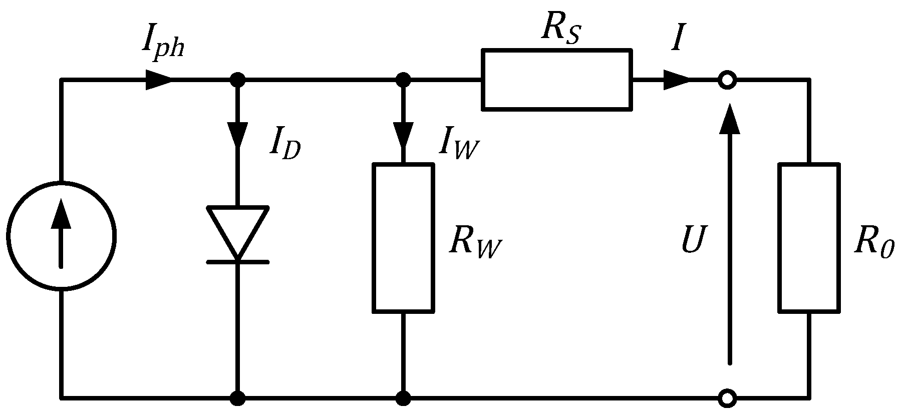
The temporal parameters of the equivalent circuit of the photovoltaic panel are critical to estimate panel inefficiency and its changes in time. The operation conditions for photovoltaic panels are usually of random nature, as discussed in [5] or in [1], as well as [19]. The randomness must be included in the panel’s equivalent models, as proved in [20]. The most popular deterministic equivalent model for photovoltaic panels is the electric circuit presented in Figure 1.
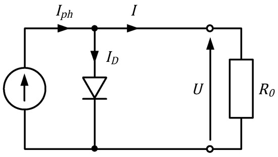
Figure 1.
Ideal equivalent circuit for a photovoltaic cell model with three parameters [21,22]: (Ω)—load resistance, (A)—current in the cell exposed to solar radiation, (A)—current in the diode with large surface area, (A)—load current, (V)—voltage decrease in the receiver.
When (A) stands current of the diode field-free, for the elementary charge (1.6∙10−19 C), is a Boltzmann constant (1.38∙10−23 J/K), (°C) is the temperature, (°C), the output current has the following value [5,21,22]:
With the increase of the temperature T, the voltage in the open circuit of the photovoltaic cell decreases. Still, the short circuit current value remains unchanged, which can be observed, in practice, as a decrease in cell power [5,23].
The Equation (2) for a photovoltaic cell, with five parameters, takes the following form [20,21,24,25]:
The corresponding equivalent circuit is presented in Figure 2.

Figure 2.
Equivalent circuit for a photovoltaic cell model with five parameters [25]: (Ω)—load resistance, (A)—current in the cell exposed to solar radiation, (A)—current in the diode with large surface area, (A)—load current, (A)—shunt resistance current, (V)—voltage decrease in the receiver, —series resistance, —shunt resistance. Reprint with permission [25]; Copyright 2005, Computer Applications in Electrical Engineering: Poznan, Poland.
Operation of the equivalent circuit in random conditions can be illustrated by assigning random values of the parameters of a single photovoltaic cell. The resultant current and voltage are the sums of the current, for the parallel circuit and the voltage values of individual cells, for the series circuit.
Using the constant randomization method in Equations (1) or (2) leads to obtaining the probabilistic characteristics of the photovoltaic cell. If the temperature changes randomly, the relation obtained for the Equation (1) is:
where:
and is a stochastic process.
Due to the undisclosed dependencies described and captured in the equations above, the equations obtained are inaccurate. A better model of the photovoltaic cell inefficiency is obtained through the rolling comparison with the averaged model based on performed measurements. These measurements can be done for a non-defective module. The method proposed for the analysis is based on the definition of the processed residual.
3.2. Modification of the Residual Method
There are many residual definitions, including those that are pseudo-residual. In the simplest residual assessment method, the result of measurements designated as is compared with the signal generated by the model, generating the residual (ordinary residuals) [25,26,27,28,29]:
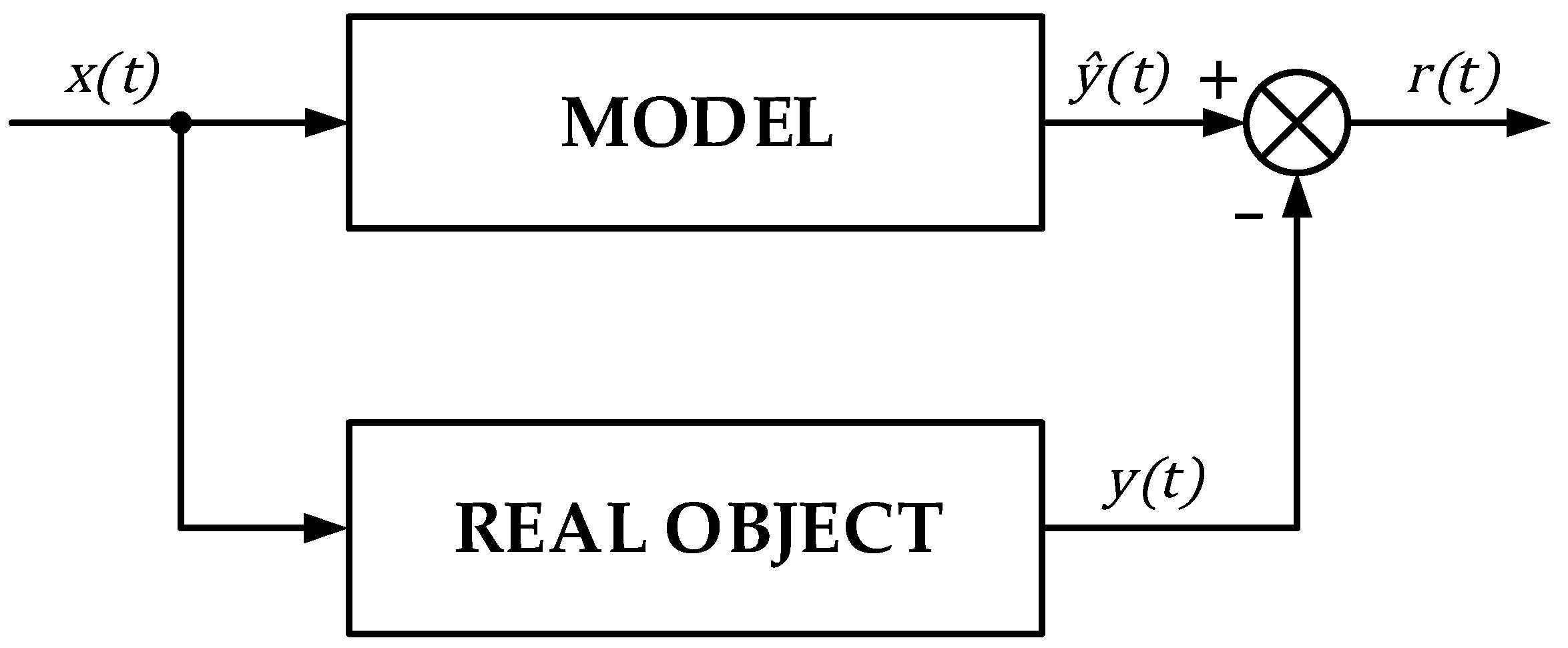
When the object operates correctly, the residual value should be zero, and it should be different from zero as soon as a failure or inefficiency appears (Figure 3).

Figure 3.
Ideal scheme for the residual assessment method: —enforcements, in a given moment in time.
Residual values different than zero are also observed when the following conditions occur [29,30,31,32]:
- model inaccuracies of linear nature, for example, in the sectional function of the output signal,
- interferences in the actual random measurement values.
As a result of these, it is necessary to establish a certain area of model uncertainty for residual values around [33].
A more objective mapping of the current residual value onto the state of the non-linear object under examination can be obtained through the conversion of the residual absolute value to the relative value (%) [34]:
or more accurately:
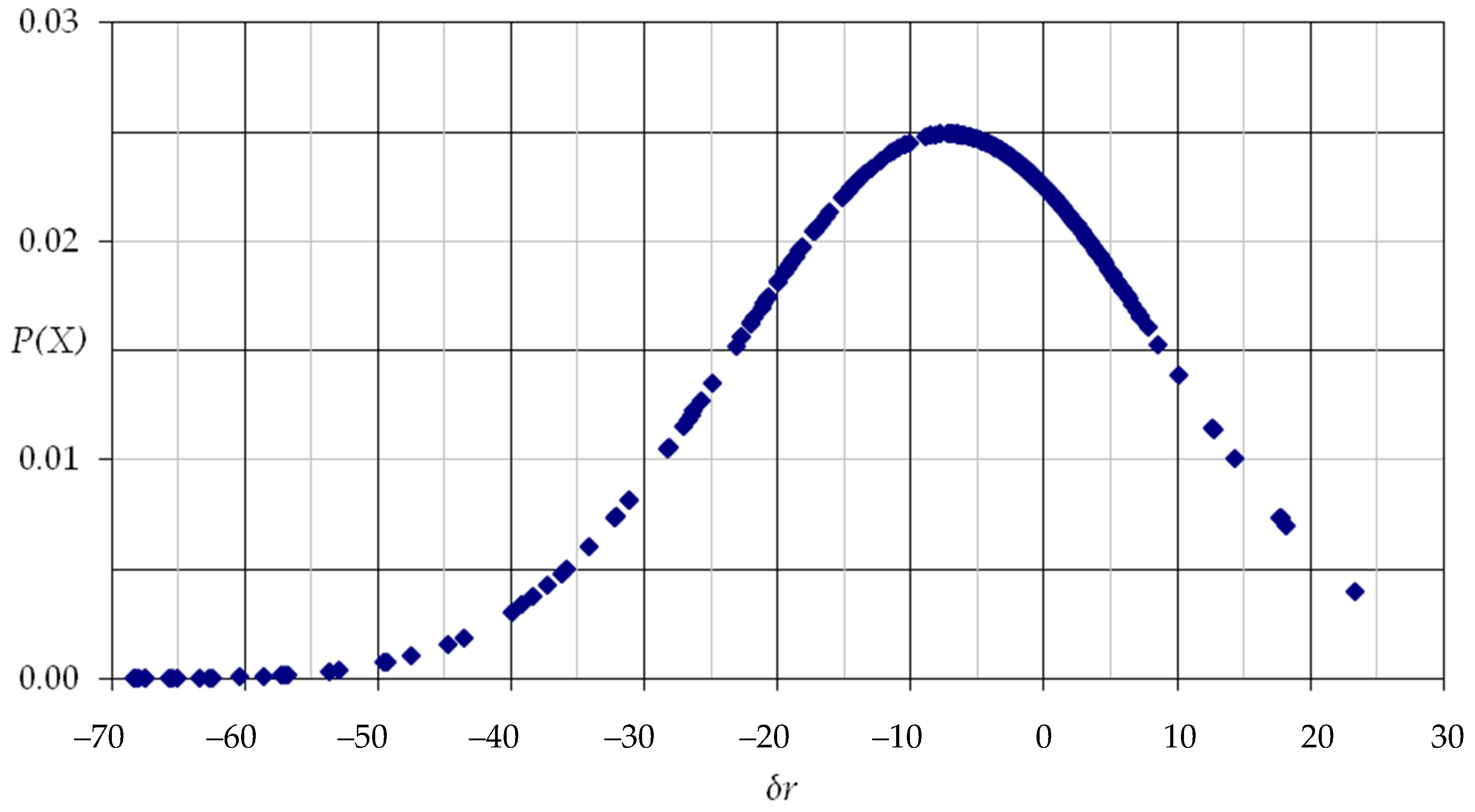
Relative residual values guarantee a more accurate assessment of the current state regarding quality and quantity. It can be assumed that residuals are variables randomly subject to the Gauss normal distribution P(X) [35]. This is confirmed by the curve obtained from measurements and calculations (as shown in Figure 4), determined based on experimental data from the cell load range of 0–200 Ω and its final model. The modeling error is represented as the displacement of the bell curve peak to the left of the ideal value .
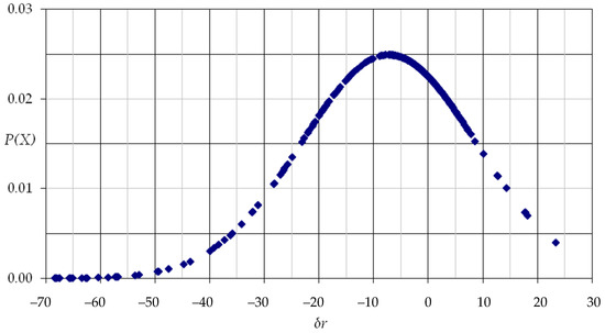
Figure 4.
Gauss Curve for relative residual distribution during modeling [24]. Reprint with permission [24]; Copyright 2010, Poznan University of Technology: Poznan, Poland.
A residual method is then modified by introducing the dynamic determination of alarm limits by appropriately transforming the measured values. Temporal values are transformed into discrete while residual signals (—measurement number) are transformed using the following equation [31,33,36]:
where: —residual value after the modification, —standard deviation estimate for historical data about correct object operation from the , which absolute values (7) were higher than the standard deviation estimate calculated for all the data:
where: —mean value of all values, —the number of , which absolute values were higher than the standard deviation estimate , —the number of all values.
As a result, the modified discrete values of in the applied inference methods reduce the impact of too large residual values obtained in the case of the correct operation of the evaluated (diagnosed) system. The authors also use modifications similar to (8) in their considerations concerning, e.g., diagnostics of the machine condition with the use of artificial intelligence, e.g., in the group data processing method (in GMDH neural networks) [31], in the preparation of data sets in fuzzy modeling [33], in fault detection using autoregressive (ARV) models [37].
3.3. Assessing Photovoltaic Cell Wear/Defects
Residual values greater than zero after modification can indicate a defect in the object under examination, but they can also signal other states. The processed residuals are subject to averaging in the next stage by determining moving average values with the dynamically calculated time horizon for every discrete-time instant :
An example of using the random signal moving average to reduce the fast-changing component of this signal, which may interfere with the application of specific methods of studying system properties, can be found in [37,38]. In [38], the random signal was a derailment coefficient used to assess the running safety of railway vehicles. In contrast, in [37], the random signal was the degree of damage to the mechanical systems tested in a laboratory.
After empirical verification, a 2-stage range of the horizon regulation was assumed. The default value is 5, but when the condition (12) is satisfied, the value is 10. The assumption of two possible values of the time horizon aims to simplify and shorten the process of calculations and inference about the state of the tested PV module. It has been verified empirically that the development of this relationship to the level of e.g., a linear function does not significantly improve the obtained results. The total number of available data points does not affect the value of in this case. Constrain (12) means that if the value for a single relative residual (6) is higher than the standard deviation determined for all the relative residuals given during normal operation, the time horizon in step is 10; otherwise, it is 5 [39].
The decisive component (12) effectively limits the consequences of temporary changes in residual values caused by random factors, as has been empirically confirmed. Such a use of moving average to reduce the random components of the investigated quantities before their further analysis is often used in technical applications, such as the safety assessment in railway vehicles [38].
It is assumed that the limit is proportional to the model inaccuracy in a given discrete-time instance :
where: —standard deviation estimate in the given time horizon —for the original residuals .
Finally, the condition revealing defect, wear, or other disturbance for the detection of inefficiency is obtained:
where: —estimation of the residual standard deviation caused, for example, by a defect of the monitored object, —estimation of the standard deviation for residuals caused by the inaccuracy of the model.
Finally, the modified inference based on Formulas (13) and (14) may lead to more accurate models formulated with the use of multivariable function approximation, reflecting the operation of diagnosed systems [39].
Satisfying the condition (14) does not constitute the complete diagnosis of the module’s damage. However, it is a premise for further verifying the assessment to determine the seriousness of the inefficiency.
The initial assessment is suggested to be verified by establishing whether the value fits within the power range assumed for the panel’s operation.
According to the different studies on the subject [40,41], the standard practice is to use modules mostly in the generated power range , and more rarely in . Furthermore, while the module is in operation, in the range of high declining steepness of the characteristics below , even a small change in the load and the random environmental conditions (e.g., temporary shading) can generate false, high-value residuals. That is why the verification in the broader range of power fluctuations should confirm the final assessment of the module inefficiency. Whether a given measurement series falls into that range is determined by checking the condition. The condition is checked using the mathematical model of the power sample for the range specified above, which is also determined using the model.
The modifications introduced a “smooth” assessment of the condition of the photovoltaic cell. Thus, they can help prevent temporary false alarms. Unfortunately, they also cause an additional time delay in detecting the wear or defect state. Considering long exploitation periods for photovoltaic modules when they reach 90% of the rated power, as specified by the manufacturer, a slight delay in the diagnostic decision should not increase economic losses.
In the course of the research, it turned out that the inefficiency (wear) state of a photovoltaic module at the -th moment is directly proportional to the percentage average of the relative residual value:
where: means satisfaction of all the conditions and performing calculations in the 10 last discrete steps .
Based on the empirical dependencies given by the histograms, it is assumed that the average relative residual value is calculated from the last steps providing that the time horizon does not change in those consecutive steps. Furthermore, the average value (16), must be characterized with the standard deviation , which is no higher than 20% of the average value module while condition (14) must be satisfied for the given set of samples measured [34]:
Satisfying the detection condition (15) makes it possible to minimize the influence of individual serious errors resulting from local model inaccuracies or random faults in the measurement samples. A value of the parameter, greater than zero, can indicate that the cell is wearing out. Inaccuracies can cause a parameter value smaller than zero in the measurements or by the model itself.
4. Results and Discussion
4.1. Verification of the Inefficiency Detection Method
The proposed detection method has been verified empirically on random measurement samples in the actual operating conditions of the module. Parameters (real value) and (model value) in equation (6) have been substituted with the equivalent current values and .
Initial tests were carried out in the laboratory, but the primary tests of the PV module were performed outside buildings in Poznan (latitude: 52.4 °N, longitude: 16.95 °E). Poznan is located in a temperate climate zone, transitioning from a maritime climate to a continental climate. As a rule, the weather here is variable, with the average annual rainfall about 507 mm, which is 30% less than the average for the whole country. The Shell ST20 module, made of amorphous cells, was approximately three years old at the time of the measurements, but it had been previously tested for over two years. In the described case, the modeling and condition evaluation process was performed on the PV module itself. The module’s characteristics were determined by measuring the current and voltage at its terminals during manual changes in the load resistance. The tested system was not equipped with an inverter. Moreover, the stability of the ambient temperature and the wind speed was monitored during the measurement series under the given radiation intensity conditions.
Voltage and current measurements were planned to concentrate measurements in the vicinity of the maximum power point—MPP (±10% of the value of the estimated UMPP voltage). Concentration resulted from changing load resistance to obtain four times more measurement samples on the performance characteristics. The examination started from less precise measurement and determination of the characteristics (with points evenly distributed on the curves). Current-voltage and power under given conditions, and subsequently the location of the maximum power point, were empirically determined. Then the characteristics with the concentration of measurements mentioned above were measured and picked near the MPP point. In standard installations, the PV modules work close to the MPP point, which the inverter fulfils.
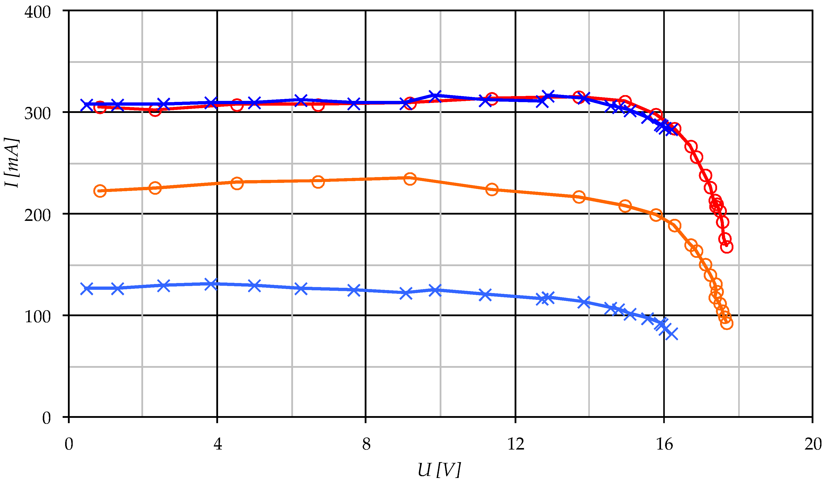
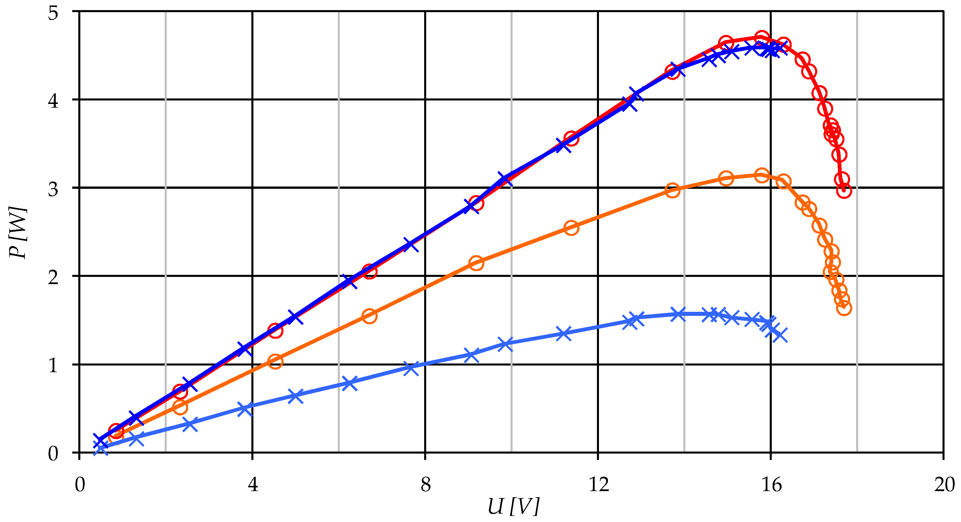
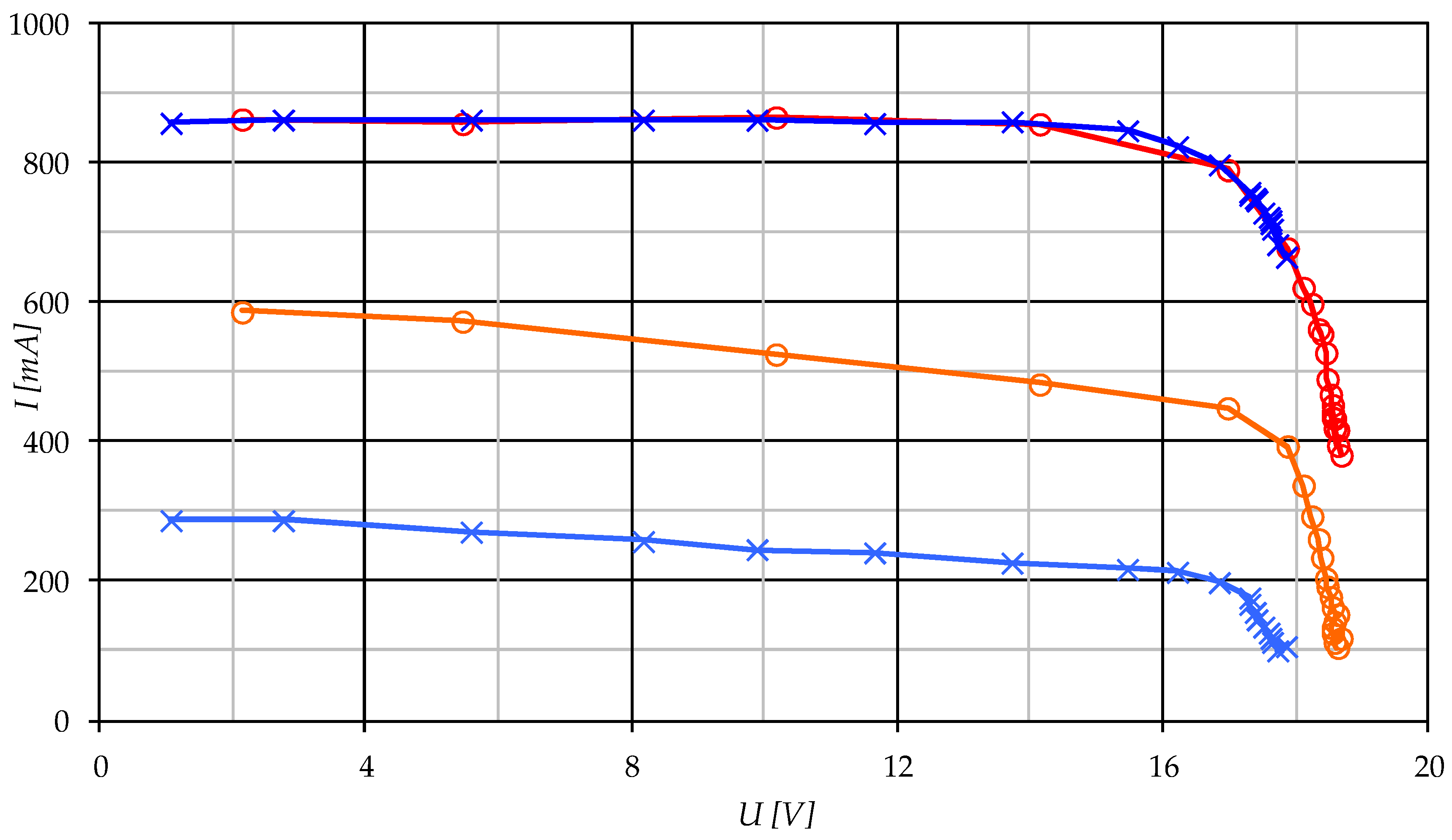
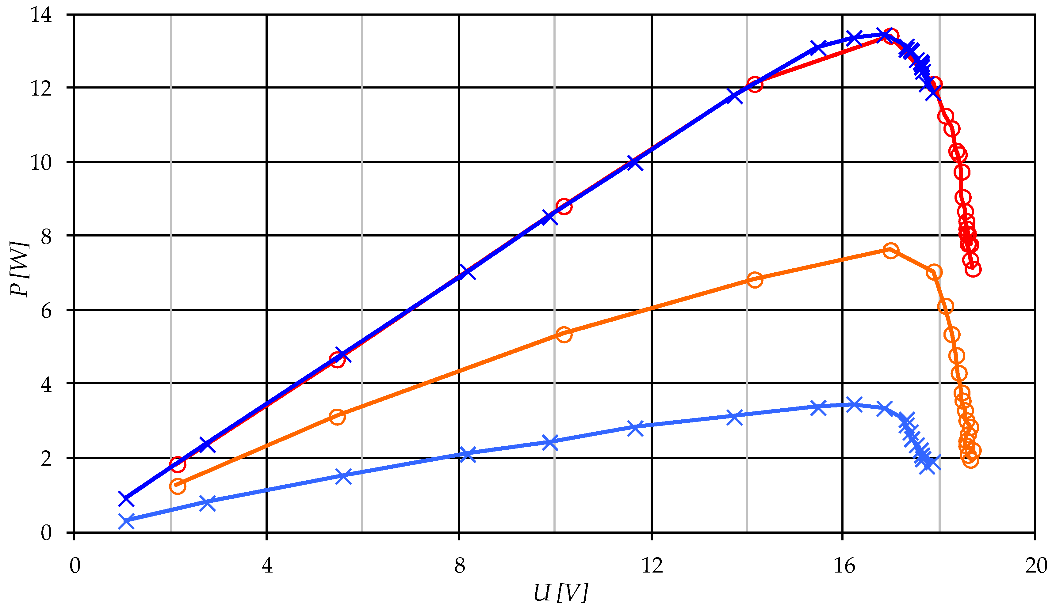
Figure 5 shows the influence of random shading of the module’s working surface on the current-voltage characteristics of its operation in the load range from 0 to 200 Ω for irradiation 200–210 W/m2. The relation between power and voltage was obtained in the same way (Figure 6).
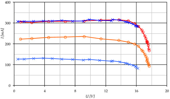
Figure 5.
Sample characteristics of a photovoltaic module (200–210 W/m2), curves: red, dark blue—model values for a fully operational module, orange—real values with the blind covering 30% of the module surface, light blue—real values with the blind covering 60% of the module surface.
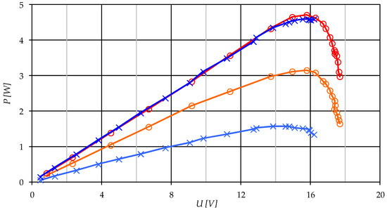
Figure 6.
Sample characteristics of a photovoltaic module (200–210 W/m2), curves: red, dark blue—model values for a fully operational module, orange—real values with the blind covering 30% of the module surface, light blue—real values with the blind covering 60% of the module surface.
Differences between the model curves (red and dark blue in Figure 5 and Figure 6) result mainly from small differences in temperature during the two series of measurement. The measurements done with 60% shading of the module working surface were performed when the temperature was about 2 °C higher, although the lighting conditions were very similar and amounted to about 200–210 W/m2.
Some interferences were modeled with the use of blinds. Shading a part of the module’s surface simulates a failure of the part of the cell that caused by different external factors and wear [23]. Multiple measurements repetitions for randomly shaded areas of the module have shown that the placement of the blind on a correctly operating photovoltaic module does not play any role in the results obtained.
- average malfunction levels calculated for samples from the whole power fluctuation range , without satisfying condition (15) in their selection, the results obtained amounted to respectively: 2.716% with no blind, 34.897% with a 30% blind and 62.806% with a 60% blind,
- analogously to the above, the average values obtained when condition (15) was satisfied were as follows: 0% with no blind, 32.627% with a 30% blind, and 57.497% with a 60% blind.
The results obtained confirm the usefulness of condition (15) in the precise determination of the malfunction state, as using this criterion reduces the scatter band for the malfunction state around the expected values.
Figure 7 and Figure 8 show the influence of shading random areas of the module’s working surface on the current-voltage characteristics (Figure 7) and power-voltage characteristics (Figure 8) in the load range from 0 to 200 Ω for irradiation 490–560 W/m2. There is a noticeable and proportional increase in the current and power curves value due to the higher level of irradiation.
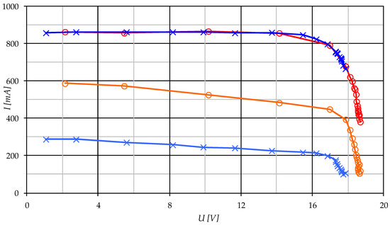
Figure 7.
Sample characteristics of a photovoltaic module (490–560 W/m2), curves: red, dark blue—model values for a fully operational module, orange—real values with a blind covering of 30% of the module surface, light blue—real values with a blind covering of 60% of the module’s surface.
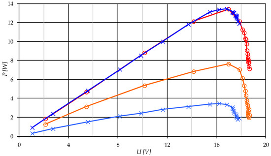
Figure 8.
Sample characteristics of a photovoltaic module (490–560 W/m2), curves: red, dark blue—model values for a fully operational module, orange—real values with a blind covering of 30% of the module surface, light blue—real values with a blind covering of 60% of the module’s surface.
Table 1 shows similar values of the malfunction state obtained for other levels of the radiation power density .

Table 1.
Sample malfunction state values for different irradiance values for the full range of power variations.
Analysis of the results, such as presented in Table 1, made it possible to improve the malfunction state assessment, considering the detection condition (15). It was also revealed that malfunction state values decrease in the direction of the actual percentage of the blind use. The results presented above pertain to the whole range of variations for the characteristics examined, and Table 2 shows comparable results for the power range of .
Table 2.
Sample values of the malfunction state for different irradiance values for .
The sample data sets presented in Table 2 show that for the power range of , the errors in malfunction state assessment have decreased in number and amount to zero for module operation without blinds considering the detection condition (15).
Summing up, the sets of graphs obtained and presented in Figure 5, Figure 6, Figure 7 and Figure 8 do not guarantee the complete assessment of the state/degree of malfunction/dirt/shade, but in combination with irradiation measurement and the methodology proposed in the paper, allow estimating the state of tested PV module. Table 1 and Table 2 calculated the estimated degrees of failure. Table 2 narrowed the inference to the power range , which allowed for more satisfactory results, especially in the absence of a curtain (“No blind” column).
The measurement uncertainty was minimized during the tests using 8 HT204 irradiation meters distributed evenly around the tested PV module. The reliability of the measurements was verified with a photometer/radiometer Ee-Meter 202 with pyranometer CM11. The indicated range of changes, e.g., 490–560 W/m2, refers to the extreme values of irradiance indicated by different, mostly farthest from each other, probes of HT204 m. The mean value of the readings from all meters was satisfactorily (error of ±1.5%) with the value indicated by the Ee-Meter 202. The original measurement error of each HT204 is ±5%; however, it was reduced to ±1.5% in practice. For the variability range of the irradiance of 490–560 W/m2, the average from the series of 30 measurements taken during 180 s was 522 W/m2. This value was determined with an accuracy of ±1.5%, meaning 522 ± 7.83 W/m2. For other given ranges of irradiation, the measurement errors were respectively: ±1.25% for Dr = 120–150 W/m2, ±1.05% for Dr = 200–210 W/m2 and ±1.35% for Dr = 370–400 W/m2.
4.2. Establishment and Analysis of Periodic Malfunctions from Diagnostic Data
In the current analysis of temporary inefficiencies, using Formula (6) and the assumption of the stochastic nature of the recorded data, it was decided to schedule them under random time intervals. The temporary failure at the discrete time j is given by the formula:
where: —measured current value after conversion, real current value (from the measurement at the discrete moment) [mA], —the current value generated by the model at the discrete moment [mA]. The interval between consecutive discrete moments is regulated, and the specific value of is an estimate (as arithmetic mean) of ten consecutive values calculated with the assumed frequency of one value per second (according to the condition (15) of modification of the residual method). Therefore, the time interval between successive calculated values of should meet the condition:
where: , —beginning and end of period for calculating the next ten values.
Depending on the time interval the sample size of the failure values collected over a given time series can vary. The test assumes a fixed unit period of the time series equal to month. In practice, this period is the time interval between successive values of periodic inefficiencies calculated from the set and recorded in the database. The calculation of periodic failures is preceded by the determination of the central moment of the second order—variance [%2] defined by the formula:
where: —estimate (first order of the central moment), arithmetic mean of temporary failures in the time interval [%].
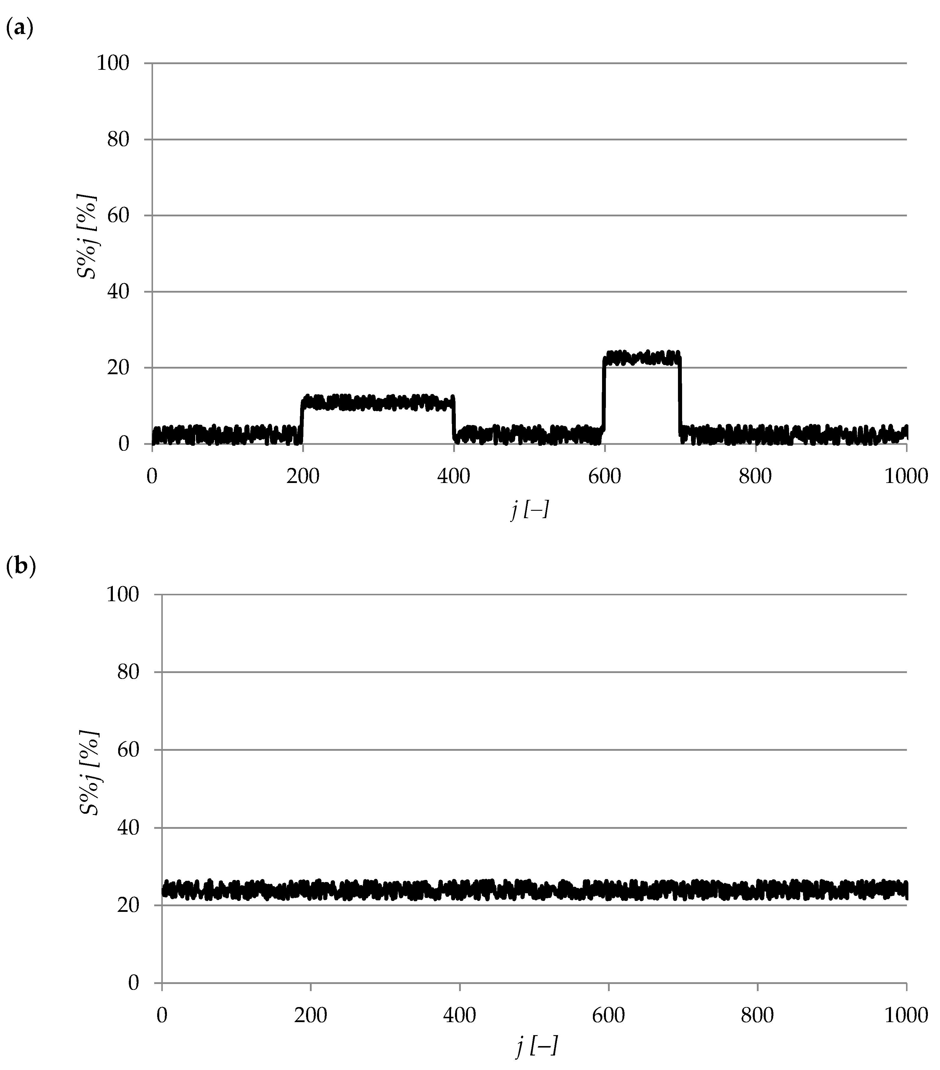
For further consideration, the inefficiency of the tested module was simulated by randomly located diaphragms on the working surface of the amorphous module. The measurements were carried out according to previous assumptions. However, temporary failure was calculated every min. Time interval was shortened to the first week, therefore within one period 1008 designated values were archived and subjected to further mathematical analysis. Cases without fluctuations and with short-term random fluctuations increasing the variance [24] and, consequently, the necessity of marking and analysing the histograms were taken into account. Figure 9 presents courses of failure in consecutive discrete moments ( samples). In contrast Figure 10 shows histograms in two cases: —during damage-free operation (without aperture) with random shadows, —when working with a randomly located aperture 24% of the working surface of the module.

Figure 9.
characteristics: (a) ; (b) .

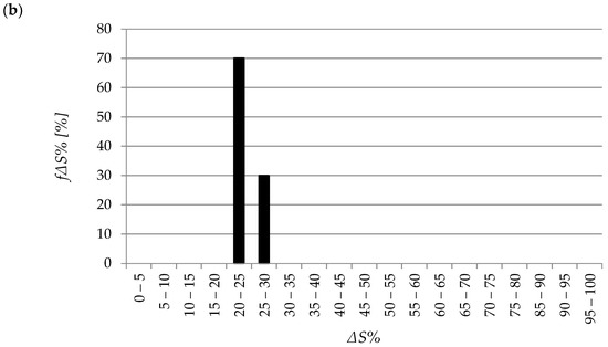
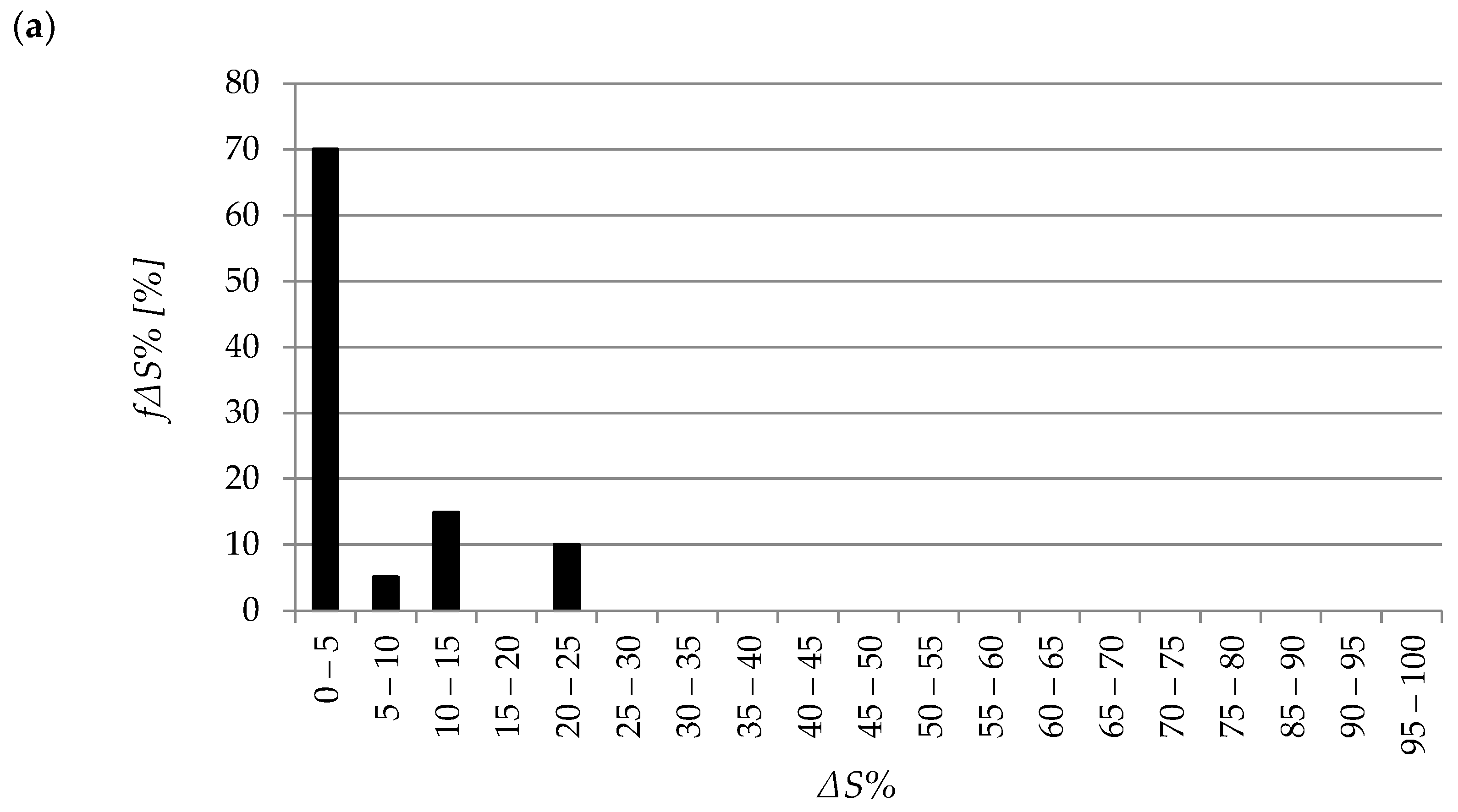
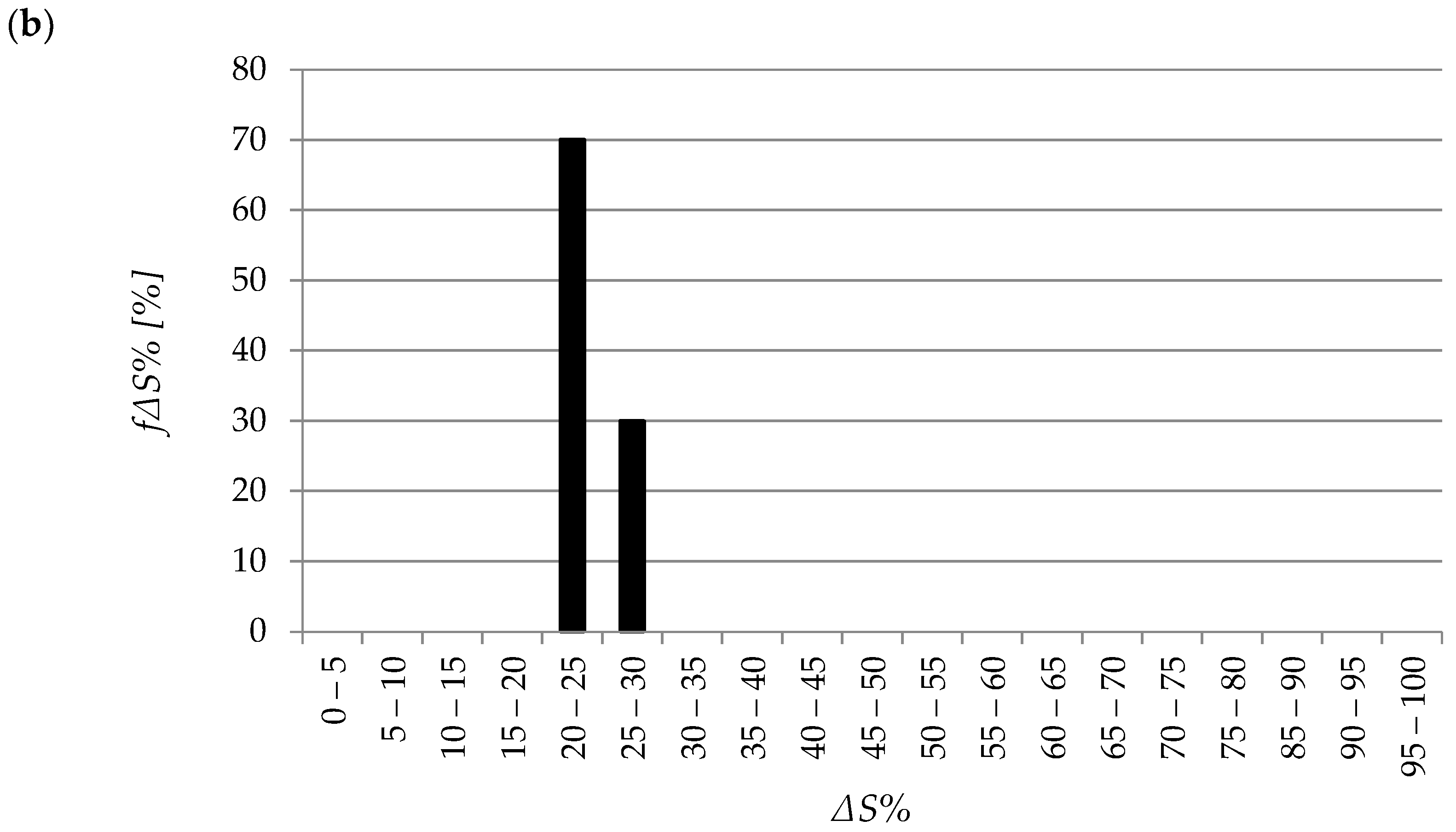
Figure 10.
Histograms : (a) ; (b) .
For greater clarity of the results, it was decided to draw up histograms in which the height of the bars is proportional to the relative size (percentage) of a given interval in relation to the entire population. Relative abundance is expressed as percentage .
In case a, the presence of temporal shadows was noted (for successive discrete-time moments and ) with random unknown values, as confirmed by the histogram (Figure 10a) with a clear dominance of the bar of the malfunction in the and a high value of the variance equal to 43.09%2.
In case b with the shutter in Figure 9b, the uniformity of the inefficiencies, as observed over time, is confirmed by the very low variance value at the level of 1.89%2.
To minimize the impact of randomly changing working conditions on the value of periodic failure , it was proposed to introduce a failure stability criterion in the period.
Empiria confirmed that a variance not exceeding 5% proves a sufficiently stable course of the instantaneous values and entitles the periodic inefficiency to be calculated as estimates (arithmetic mean) of all in time interval without considering the histogram. A variance value higher than 5% obliges to proceed according to the scheme described by the formula:
where: —probabilistic weighting factor depending on the relative size (percentage) of the failure interval and variance values [%].
It comes down to determining the as the expected value, using the histogram (Figure 10) and the weighting factors depending on the relative size (percentage) of the failure interval and the variance value according to the formula:
where: —the number of bars lower than the average height in the histogram. The value of the weighting factor is determined for each interval separately. However, their sum over all intervals must be equal to 100%. The first case (Formula 20) concerns the weighting factors for histogram bars higher than the average of all bars , and the second case concerns the coefficients for the remaining bars lower than the mean value. A similar use of weighting factors depending on the random quantities that exceed their limit values at some discrete moments has been applied in the statistical analysis of the track irregularities that temporarily reduce the running safety and ride comfort of railway vehicles [38].
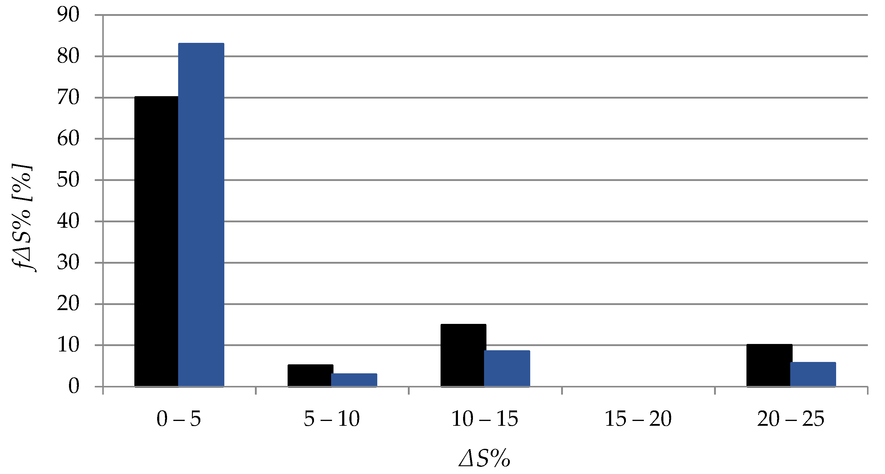
Figure 11 shows a comparison of the original histograms (from Figure 10a) with those modified according to the Formula (21), where the new values of are equal to the determined weighting factors .

Figure 11.
Comparison of original (black) and modified (blue) histograms for .
Table 3 confirms the validity of the application of the criterion of the disability stability, in the period when determining the periodic failure .
Table 3.
Comparison of the results of determining periodic failure of using the estimation and weighting method.
Due to the possibility of the fluctuations mentioned above, attention should be paid to their influence in the monitoring process, especially concerning seasonal changes or long-term accidental fluctuations. In such a case, applying the methodology described above does not give measurable effects, even in the case of increasing the considered time windows, because in the longer horizon, there are too many random factors of different duration that can be omitted by the method.
The investigations of the PV module presented in this work are a substantial contribution to assessing their reliability and can be helpful in their maintenance. These two issues and efficient energy use are vital aspects in many engineering applications.
5. Conclusions
The argumentation and verification results presented above (Table 1 and Table 2) confirm the usefulness of assessing the malfunction’s state, as developed by the authors. It is useful when assessing the condition (malfunction state) of amorphous modules characterized by the most significant random changes of operation parameters. For this reason, the method was developed and confirmed through tests using the Shell ST20 amorphous module. The usefulness of the method has been demonstrated particularly during the verification of the mathematical model.
The verification process allowed to determine periodic inefficiencies of the tested PV module. Based on the residual method described in the paper and modified by the authors, a variance was used to prepare histograms determining the percentage belonging to the designated intervals. The methodology of creating histograms was also modified by applying a probabilistic weighting factor. The factor allows short-term fluctuations (changes in tested signal) affecting the final state (malfunction) assessment to be eliminated. As seen in Section 3.2, implementing the histograms using the variance allows even better approximation of the value of the estimated failure of the PV module to the real value. It is visible as an increase in the value of the histogram ∆S% = 0–5 in Figure 11 by almost 13%. Applying this additional inference method in the presented case of lack of shading (0%) decreased the estimated inefficiency S%SC from 6.1% to 0.9% (Table 3), i.e., it came closer to the real value. The presented methodology was verified in assessing the state of failure of PV modules, which mathematical models were previously derived from model measurement data in the approximation process [24]. The results confirm the effectiveness of the adopted concept of dealing with the stochastic nature of working conditions, dynamically changing over relatively short periods. With random, unpredictable long-term changes (e.g., seasonal), the proposed modification strategy of the methods described does not allow more accurate state results to be estimated due to the failure of the PV module tested. This is due to the influence of too many randomly changing factors of varying duration, occurring at varying time intervals.
Further research will take into account the influence of the inverter Maximum Power Point Tracker, temperature changes, and the influence of wind speed. In addition, the proposed methodology will be enriched with an algorithm recognizing long-term, slow-varying shading of predictable origin (e.g., from structural elements of the building, other PV modules, trees). This will allow predicting (estimating) the geometry and, at the same time, the scope of the occurring shading and, thus, recognizing its potential sources.
Author Contributions
Conceptualization, G.T., J.J., N.C.-G., E.K.-C. and W.W.; methodology, G.T. and J.J.; software, G.T. and J.J.; validation, G.T., J.J., N.C.-G. and W.W.; formal analysis, G.T., J.J., N.C.-G., E.K.-C. and W.W.; resources, G.T., J.J., N.C.-G., K.L. and W.W.; data curation, G.T. and J.J.; writing—original draft preparation, G.T. and J.J.; writing—review and editing, G.T., J.J., N.C.-G., E.K.-C., K.L. and W.W.; visualization, G.T. and J.J.; supervision, N.C.-G., K.L. and E.K.-C.; funding acquisition, E.K.-C. and K.L. All authors have read and agreed to the published version of the manuscript.
Funding
The research received financial support from the Scientific Council of Civil Engineering and Transport at Warsaw University of Technology.
Institutional Review Board Statement
Not applicable.
Informed Consent Statement
Informed consent was obtained from all subjects involved in the study.
Data Availability Statement
Data available in a publicly accessible repository.
Acknowledgments
The authors would like to gratefully acknowledge the reviewers that provided helpful comments and insightful suggestions on a draft of the manuscript.
Conflicts of Interest
The authors declare no conflict of interest. The funders had no role in the design of the study; in the collection, analyses, or interpretation of the data; in the writing of the manuscript; or in the decision to publish the results.
Nomenclature
| PV | Photovoltaic |
| R0 | Load resistance |
| Iph | Current in the cell exposed to solar radiation |
| ID | Current in the diode with large surface area |
| I | Load current |
| U | Voltage decrease in the R0 receiver |
| I0 | Current of the diode field-free |
| q | Elementary charge |
| kB | Boltzmann constant |
| T | Temperature |
| IW | Shunt resistance current |
| RS | Series resistance |
| RW | Shunt resistance |
| T(t) | Stochastic process |
| y | Result of measurements in the simplest residual assessment method |
| Signal generated by the model | |
| r | Residual |
| δr | Relative value of residual |
| P(X) | Gauss normal distribution |
| Rj | Residual value after the modification, estimation of the residual standard deviation caused, for example, by a defect of the monitored object |
| σz | Standard deviation estimate for historical data about correct object operation from the |
| σw | Standard deviation estimate calculated for all the data |
| gj | Determining moving average values |
| Nj | Dynamically calculated time horizon for every j |
| j | Discrete-time instant |
| lj | Estimation of the standard deviation for residuals caused by the inaccuracy of the model |
| Standard deviation estimate in the given time horizon for the original residuals | |
| S%j | Inefficiency (wear) state of a photovoltaic module at the -th moment, the estimate (as arithmetic mean) of ten consecutive values |
| n | Number of last discrete steps |
| Standard deviation characterizing the average value | |
| MPP | Maximum power point |
| Dr | Radiation power density |
| S% | Malfunction state value |
| The current value generated by the model at the discrete moment | |
| Ij | Real current value (from the measurement at the discrete moment) |
| S%r | Values of inefficiency calculated with the assumed frequency of one value per second (according to the condition (15) of modification of the residual method) |
| Time interval between successive calculated values of | |
| , | Beginning and end of period for calculating the next ten values |
| Values of periodic inefficiencies calculated from the set and recorded in the database | |
| Central moment of the second order—variance | |
| Estimate (first order of the central moment), arithmetic mean of temporary failures in the time interval | |
| Probabilistic weighting factor depending on the relative size (percentage) of the failure interval and variance values | |
| Relative size (percentage) of the failure interval | |
| nf | Number of bars lower than the average height in the histogram |
References
- Głuchy, D.; Kurz, D.; Trzmiel, G. The impact of shading on the exploitation of photovoltaic installations. Renew. Energy 2020, 153, 480–498. [Google Scholar] [CrossRef]
- Bugała, A.; Zaborowicz, M.; Boniecki, P.; Janczak, D.; Koszela, K.; Czekała, W.; Lewicki, A. Short-term forecast of generation of electric energy in photovoltaic systems. Renew. Sustain. Energy Rev. 2018, 81, 306–312. [Google Scholar] [CrossRef]
- Zhang, C.X.; Shen, C.; Wei, S.; Zhang, Y.B.; Sun, C. Flexible management of heat/electricity of novel PV/T systems with spectrum regulation by Ag nano fluids. Energy 2021, 221, 119903. [Google Scholar] [CrossRef]
- Tomczewski, A. Operation of a Wind Turbine-Flywheel Energy Storage System under Conditions of Stochastic Change of Wind Energy. Sci. World J. 2014, 2014, 643769. [Google Scholar] [CrossRef] [Green Version]
- Skoplaki, E.; Palyvos, J.A. On the temperature dependence of photovoltaic module electrical performance: A review of efficiency/power correlations. Solar Energy 2009, 83, 614–624. [Google Scholar] [CrossRef]
- Zhang, C.X.; Shen, C.; Yang, Q.R.; Wei, S.; Lv, G.Q.; Sun, C. An investigation on the attenuation effect of air pollution on regional solar radiation. Renew. Energy 2020, 161, 570–578. [Google Scholar] [CrossRef]
- Zhang, C.X.; Shen, C.; Wei, S.; Wang, Y.; Lv, G.Q.; Sun, C. A review on Recent Development of Cooling Technologies for Photovoltaic Modules. J. Therm. Sci. 2020, 29, 1410–1430. [Google Scholar] [CrossRef]
- Ali, E.M.; Abdelsalam, A.K.; Youssef, K.H.; Hossam-Eldin, A.A. An Enhanced Cuckoo Search Algorithm Fitting for Photovoltaic Systems’ Global Maximum Power Point Tracking under Partial Shading Conditions. Energies 2021, 14, 7210. [Google Scholar] [CrossRef]
- Darussalam, R.; Pramana, R.I.; Rajani, A. Experimental investigation of serial parallel and total-cross-tied configuration photovoltaic under partial shading conditions. In Proceedings of the International Conference on Sustainable Energy Engineering and Application (ICSEEA), Jakarta, Indonesia, 23–24 October 2017; pp. 140–144. [Google Scholar]
- Salam, Z.; Ramli, Z.; Ahmed, J.; Amjad, M. Partial shading in building integrated PV system: Causes, effects and mitigating techniques. Int. J. Power Electron. Drive Syst. 2015, 6, 712–722. [Google Scholar] [CrossRef]
- Eltamaly, A.M.; Abdelaziz, A.Y. Modern Maximum Power Point Tracking Techniques for Photovoltaic Energy Systems; Springer: Berlin/Heidelberg, Germany, 2019. [Google Scholar]
- Abolhasani, M.A.; Rezaii, R.; Beiranvand, R.; Varjani, A.Y. A comparison between buck and boost topologies as module integrated converters to mitigate partial shading effects on PV arrays. In Proceedings of the 7th Power Electronics and Drive Systems Technologies Conference (PEDSTC), Tehran, Iran, 16–18 February 2016; pp. 367–372. [Google Scholar]
- Alshareef, M.; Lin, Z.; Ma, M.; Cao, W. Accelerated Particle Swarm Optimization for Photovoltaic Maximum Power Point Tracking under Partial Shading Conditions. Energies 2019, 12, 623. [Google Scholar] [CrossRef] [Green Version]
- Zhang, C.X.; Shen, C.; Yang, Q.R.; Wei, S.; Sun, C. Blended Ag nanofluids with optimized optical properties to regulate the performance of PV/T systems. Solar Energy 2020, 208, 623–636. [Google Scholar] [CrossRef]
- Kaminski, K.; Znaczko, P.; Lyczko, M.; Krolikowski, T.; Knitter, R. Operational Properties Investigation of the Flat-Plate Solar Collector with Poliuretane Foam Insulation. Procedia Comput. Sci. 2019, 159, 1730–1739. [Google Scholar] [CrossRef]
- Alawi, O.A.; Kamar, H.M.; Mallah, A.R.; Monhammed, H.A.; Sabrudin, M.A.S.; Newaz, K.M.S.; Najafi, G.; Yaseen, Z.M. Experimental and Theoretical Analysis of Energy Efficiency in a Flat Plate Solar Collector Using Monolayer Graphene Nanofluids. Sustainability 2021, 13, 5416. [Google Scholar] [CrossRef]
- Alawi, O.A.; Kamar, H.M.; Monhammed, H.A.; Mallah, A.R.; Hussein, O.A. Energy efficiency of a flat-plate solar collector using thermally treated graphene-based nanofluids: Experimental study. Nanomater. Nanotechnol. 2020, 10. [Google Scholar] [CrossRef]
- Kuczynski, W.; Kaminski, K.; Znaczko, P.; Chamier-Gliszczynski, N.; Piatkowski, P. On the correlation between the geometrical features and thermal efficiency of flat-plate solar collectors. Energies 2021, 14, 261. [Google Scholar] [CrossRef]
- Wang, L.; Lin, Y.H. Random fluctuations on dynamic stability of a grid-connected photovoltaic array. IEEE Power Eng. Soc. Winter Meet. 2001, 3, 985–989. [Google Scholar] [CrossRef]
- Trzmiel, G. Determination of a mathematical model of the thin-film photovoltaic panel (CIS) based on measurement data. Maint. Reliabil. 2017, 19, 516–521. [Google Scholar] [CrossRef]
- Kerr, M.; Cuevas, A. Generalized analysis of the illumination intensity vs. open-circuit voltage of solar cells. Solar Energy 2004, 76, 263–267. [Google Scholar] [CrossRef]
- Skowronek, K.; Trzmiel, G. The method for identification of fotocell in real time. In Proceedings of the ISTET—XIV International Symposium on Theoretical Electrical Engineering, Szczecin, Poland, 20–23 June 2007. [Google Scholar]
- Ikegami, T.; Maezono, T.; Nakanishi, F.; Yamagata, Y.; Ebipara, K. Estimation of equivalent circuit parameters of PV module and its application to optimal operation of PV system. Solar Energy 2001, 67, 389–395. [Google Scholar] [CrossRef]
- Trzmiel, G. Stochastic Analysis of the Characteristics of the Photovoltaic Module. Ph.D. Thesis, Poznan University of Technology, Poznań, Poland, 2010. [Google Scholar]
- Skowronek, K.; Trzmiel, G. Generalized analysis of the effect of statistical scatter of the elements of photovoltaic matrix on its equivalent dynamic parameters by random values of darkening fields. In Computer Applications in Electrical Engineering; Publishing House of Poznan University of Technology: Poznan, Poland, 2005; pp. 238–249. [Google Scholar]
- Korbicz, J.; Koscielny, J.M.; Kowalczuk, Z.; Cholewa, W. Fault Diagnosis: Models, Artificial Intelligence, Applications; Springer Science & Business Media: Berlin/Heidelberg, Germany, 2012. [Google Scholar]
- Cox, D.R.; Snell, E.J. A general definition of residuals. J. R. Stat. Soc. Ser. B 1968, 30, 248–265. [Google Scholar] [CrossRef]
- Loynes, R.M. On Cox and Snell’s general definition of residuals. J. R. Stat. Soc. Ser. B 1969, 31, 103–106. [Google Scholar] [CrossRef]
- Haslett, J.; Hayes, K. Residuals for the linear model with general covariance structure. J. R. Stat. Soc. Ser. B 1998, 60, 201–215. [Google Scholar] [CrossRef]
- Skowronek, K.; Trzmiel, G. Identification of photovoltaic matrix in real time. In Proceedings of the Seventh International Conference on AMTEE—Advanced Methods of the Theory of Electrical Engineering, Plzen, Czech Republic, 10–12 September 2007. [Google Scholar]
- Bartol-Smardzewska, M. Application of Artificial Intelligence in Machine Diagnostics; Diagnostyka, Polskie Towarzystwo Diagnostyki Technicznej: Warszawa, Poland, 2005; p. 33. (In Polish) [Google Scholar]
- Witkowski, K. The Possibility of Using Multivalued Evaluation of Residuals in the Diagnostics of Marine Diesel Engine; Diagnostyka, Polskie Towarzystwo Diagnostyki Technicznej: Warszawa, Poland, 2012; pp. 59–62. [Google Scholar]
- Kowal, M.; Korbicz, J. Self-organizing fuzzy Takagi-Sugeno model in the system fault detection. In Proceedings of the 6th National Scientific and Technical Conference “Diagnostics of Industrial Processe”, Władysławowo, Poland, 15–17 September 2003. (In Polish). [Google Scholar]
- Anscombe, F.J.; Tukey, J.W. The examination and analysis of residuals. Technometrics 1963, 5, 141–160. [Google Scholar] [CrossRef]
- Skowronek, K. Electrical Circuits in Stochastic Approach; Poznan University of Technology Publisher: Poznań, Poland, 2011. (In Polish) [Google Scholar]
- Pierce, D.A.; Schafer, D.W. Residuals in generalized linear models. J. Am. Stat. Assoc. 1986, 81, 977–986. [Google Scholar] [CrossRef]
- Mattson, S.G.; Pandit, S.M. Statistical moments of autoregressive model residuals for damage localisation. Mech. Syst. Signal Process. 2006, 20, 627–645. [Google Scholar] [CrossRef]
- Kardas-Cinal, E. Statistical Method for Investigating Transient Enhancements of Dynamical Responses due to Random Disturbances: Application to Railway Vehicle Motion. ASME J. Vib. Acoust. 2020, 142, 061008. [Google Scholar] [CrossRef]
- Trzmiel, G. Verifications of the photovoltaic cell models formulated with the use of multivariable function approximation. In Proceedings of the IC-SPETO—International Conference on Fundamentals of Electrotechnics and Circuit Theory, Ustroń, Poland, 20–23 May 2009. [Google Scholar]
- Gautam, N.; Kaushika, N. Reliability evaluation of solar photovoltaic arrays. Solar Energy 2002, 72, 129–141. [Google Scholar] [CrossRef]
- Pluta, Z. Solar Energy Installations; Warsaw University of Technology Publisher: Warsaw, Poland, 2003. (In Polish) [Google Scholar]

Publisher’s Note: MDPI stays neutral with regard to jurisdictional claims in published maps and institutional affiliations. |
© 2021 by the authors. Licensee MDPI, Basel, Switzerland. This article is an open access article distributed under the terms and conditions of the Creative Commons Attribution (CC BY) license (https://creativecommons.org/licenses/by/4.0/).