Big Data Analysis and Research on Fracturing Construction Parameters of Shale Gas Horizontal Wells—A Case Study of Horizontal Wells in Fuling Demonstration Area, China

Abstract

With the rapid development of computer science and technology, the Chinese petroleum industry has ushered in the era of big data. In this study, by collecting fracturing data from 303 horizontal wells in the Fuling Shale Gas Demonstration Area in China, a series of big data analysis studies was conducted using Pearson’s correlation coefficient, the unweighted pair group with arithmetic means method, and the graphical plate method to determine which is best. The fracturing parameters were determined through a series of big data analysis studies. The big data analysis process is divided into three main steps. The first is data preprocessing to screen out eligible, high-yielding wells. The second is a fracturing parameter correlation clustering analysis to determine the reasonableness of the parameters. The third is a big data panel method analysis of specific fracturing construction parameters to determine the optimal parameter range. The analyses revealed that the current amount of 100 mesh sand in the Fuling area is unreasonable; further, there are different preferred areas for different fracturing construction parameters. We have combined different fracturing parameter schemes by preferring areas. This analysis process is expected to provide new ideas regarding fracturing scheme design for engineers working on the frontline.

1. Introduction

Big data technology has gradually penetrated all areas of social production and walks of life. Although petroleum is a traditional industry, it involves many disciplines and fields, and the amount of data and information accumulated in various aspects during long-term exploration practices is vast. With the improvement of oil and gas exploration theories and technology, oil and gas exploration work is gradually moving towards big data. The combination of big data technology and the oil and gas exploration process will certainly provide important support for the rapid development of the oil and gas exploration industry [1,2,3].

Fracturing is a necessary and technical guarantee for the production enhancement and transformation of shale oil and gas reservoirs. For blocks that are ready to implement production enhancement and transformation, the preparation of an effective fracturing design plan can scientifically guide the fracturing construction of the block, facilitate production development, and maximize the overall production of the block [4]. The optimal preferred range of fracturing construction parameters is crucial in the fracturing program, as the right amount of material must be prepared prior to fracturing, while simultaneously, the right amount of fracturing construction in the area can better improve the reservoir reformation volume and gas production.

Various methods have been used to study the optimization of fracturing construction parameters [5,6,7,8,9,10,11]. Some of the more representative methods are the applied mathematical method, the mechanistic model method, and the numerical simulation drawing board method. For example, Fan et al. [8] abstracted the fracturing construction parameter optimization problem as an optimization solution problem in mathematical equations. The optimal combination of fracturing parameters is the one that maximizes the post-fracturing capacity by optimizing the values of several construction parameters that affect the production of a single well. Tang et al. and Xu et al. [9,10] developed a mechanistic model through the seepage theory of multistage fractured horizontal wells in shale gas reservoirs to simulate reservoir modification to invert the process and construction design of horizontal wells. Yan et al. [11] analyzed the fracture width, height, and length from numerical simulations with fracture construction parameters using the graphical plate method to find the optimal range of fracture construction parameters. The first two of these methods are more cumbersome and not very operable. The numerical simulation map board method is too random, as it is uncertain how accurate the fracture parameters simulated are, so the compared results are not necessarily accurate. Based on this situation, this paper proposes a construction parameter of already fractured wells and uses the big data map board analysis method to determine the range of construction parameters for fracturing new wells.

The highlight of this study is to provide new ideas for frontline engineers regarding the design of fracturing construction parameters through the big data analysis process. This is facilitated by the simplicity of understanding, operability, and high accuracy based on field-based analysis with fractured well parameters.

This study is structured as follows: Section 2 presents basic information about the data sampling blocks. Section 3 focuses on the methodology used for the data collection and analysis. Section 4 presents our analysis process. Section 5 presents our conclusions.

2. Basic Overview of Study Area

The Fuling shale gas field, in Jianghan Oilfield, is divided into the phase I and phase II production and construction areas according to the development stage. The main section of the phase I production and construction area is the Jiaoshiba structure, a faulted anticline structure with a ground elevation of 300–1000 m. Fuling is rich in shale gas resources—ranking third in China—with a distribution area of about 76,000 square kilometers, geological resources of about 12.8 trillion cubic meters, and recoverable resources of about 2 trillion cubic meters, as shown in Figure 1. The Fuling shale gas field has the characteristics of “two high” and “two good”. First, the formation pressure is high and the natural gas composition is good. The average buried depth of the gas reservoir is 2645 m, the formation pressure coefficient is 1.55, the gas methane content is as high as 98%, the carbon dioxide content is low, and there is no hydrogen sulfide. It is a deep, ultra-high-pressure, and high-quality shale gas field. The 303 horizontal wells studied in this paper are located in the phase I production and construction area [12].

3. Methodology

3.1. Data Collection

Before doing big data analysis, the parameters corresponding to the production data are to be collected. These are both horizontal well process design parameters and fracture construction parameters. Horizontal well process design parameters are selected primarily because they are all closely related to production. The larger the contact area (longer length) of the horizontal well in the reservoir, the greater the number of fractured sections, the greater the number of shot clusters, and the higher the production rate. The specific parameters collected are, therefore: the number of fracturing sections (NFS), total perforation clusters (TC), average section length (ASL), length of the horizontal section (LHS), and number of perforation clusters per section (CS). The ASL and CS are the more important evaluation parameters for horizontal well process design; ASL is the ratio of horizontal section length to the number of fractured sections (LHS/NFS), and CS is the ratio of clusters to the number of fractured sections (TC/NFS). The data collected are shown in

Table 1. Collection of process design parameters for horizontal wells.

	NFS −	TC −	ASL (m)	LHS (m)	CS −
Maximum	29	75	97	2136	3
Minimum	11	9	53	660	1
Average	19	50	50	1467	2
Number of wells		303

.

The choice of fracturing data is mainly derived from the fracturing process. Slickwater fracturing is used in the Fuling area for shale gas development. Slickwater fracturing relies on a ground-based high-pressure pumping unit to inject slickwater into the well at high speed to fracture the shale with the help of the high pressure held at the bottom of the well. To prevent the fracture from closing on its own when the pressure drops after the pump truck stops working, a proppant (quartz sand) of different mesh sizes is mixed into the injected fluid (a combination of slickwater and linear gum) after the formation is fractured, which enters the fracture together with the fluid and stays in the fracture permanently, supporting the fracture in an open state and improving the flow of oil and gas in the reservoir in the long term. At the beginning of fracturing, a certain amount of acid is usually injected to better fracture the formation. After fracturing the shale, linear gum is added to the slickwater in order to better support the fracture and travel to the far end of the fracture. The main effect is to increase the viscosity of the slickwater to increase the sand carrying capacity, and to prevent the proppant from settling and forming a sand plug during fracturing. In summary, the basic process for fracturing can be seen in the data that need to be collected for the analysis of the fracturing construction parameters, as follows: acid amount (AC), slickwater (SW), linear glue (LG), total liquid volume (TLV), 100 mesh proppant (100 MP), 40/70 mesh proppant (40/70 MP), 30/50 mesh proppant (30/50 MP), total sand quantity (TSQ), and average sand ratio (ASR). As shown in

Table 2. Collection of design parameters for the fracturing operation of horizontal wells.

	AC (m3)	SW (m3)	LG (m3)	TLV (m3)	100 MP (m3)	40/70 MP (m3)	30/50 MP (m3)	TSQ (m3)	ASR (m3)
Maximum	820	57,188	7916	65,924	502	1104	103	1709	11
Minimum	60	5427	66	5553	36	158	0	158	0
Average	424	32,299	2892	35,615	254	715	35	750	7
Number of wells		303

, TLV, TSQ and ASR, although not mentioned in the analysis, are three important evaluation parameters for the Fuling site. TLV is the sum of the injected formation fluids, i.e., AC, SW, and LG; TSQ is the sum of the injected proppant of different mesh sizes, i.e., 100 MP, 40/70 MP, and 30/50 MP; and ASR is the ratio of injected formation proppant to total fluid volume (TSQ/TLV). The ASR is the ratio of proppant to total fluid volume (TSQ/TLV), which determines how much more fluid can be injected into the formation during fracturing. The main reason why we mention more proppant here is that, based on field experience with fracturing, if more proppant goes in without sand plugging, it proves that the fractures are well supported; thus, field engineers want to support more fractures without sand plugging.

Fracturing designs are on a per-section basis and therefore need to be converted to a section basis, i.e., a ratio of fracturing parameters to the number of sections fractured (i.e., all fracturing parameters/NFS): acid amount of each section (ACS), slickwater of each section (SWS), linear glue of each section (LGS), total liquid volume of each section (TLVS), 100 mesh proppant of each section (100 MPS), 40/70 mesh proppant of each section (40/70 MPS), 30/50 mesh proppant of each section (30/50 MPS), and total sand quantity of each section (TSQS). The specific information collected is shown in

Table 3. Collection of fracturing construction parameters.

	ACS (m3)	SWS (m3)	LGS (m3)	TLVS (m3)	100 MPS (m3)	40/70MPS (m3)	30/50MPS (m3)	TSQS (m3)
Conversion	$$\begin{gathered} ACS \\ =\frac{AC}{NFS} \end{gathered}$$	$$\begin{gathered} SWS \\ =\frac{SW}{NFS} \end{gathered}$$	$$\begin{gathered} LGS \\ =\frac{LG}{NFS} \end{gathered}$$	$$\begin{gathered} TLVS \\ =\frac{TLV}{NFS} \end{gathered}$$	$$\begin{gathered} 100MPS \\ =\frac{100MP}{NFS} \end{gathered}$$	$$\begin{gathered} 40/70MPS \\ =\frac{40/70MP}{NFS} \end{gathered}$$	$$\begin{gathered} 30/50MPS \\ =\frac{30/50MP}{NFS} \end{gathered}$$	$$\begin{gathered} TSQS \\ =\frac{TSQ}{NFS} \end{gathered}$$
Maximum	34	2042	403	2479	23	57	6	86
Minimum	3	285	3	291	2	8	0	10
Average	21	1637	147	1805	13	37	2	52
Number of wells		303

.

The source of data in big data analysis is very important, and the data in this study are mainly collected and aggregated by technicians from the field fracturing command vehicle. The horizontal well design parameters are derived from the on-site fracturing logs, and their magnitudes are mainly calculated based on the geological formations and drilling design. The fracturing parameters are derived from the on-site fracturing real-time monitoring system, and the magnitude of the values is mainly monitored by the on-site flow meter.

3.2. Data Preprocessing

Due to errors during recording or storage, some data are missing, duplicated, abnormal, or incorrect such that they are not meaningful to analyze—these are called “dirty data”. There are three types of “dirty data”: missing values, duplicate values, and abnormal values. Missing values—the abovementioned main fracturing construction parameters have gaps where data should be available; duplicate values—duplicate well data appear; abnormal values—mainly refers to unreasonable horizontal well process design and fracturing parameter data. A range of fracturing construction parameters to suit the local conditions was developed based on discussions with fracturing experts at the Fuling site, as shown in

Table 4. Data conformation range.

	CS −	LHS (m3)	NFS −	ACS (m3)	SWS (m3)	LGS (m3)	TLVS (m3)	TSQS (m3)	ASR (%)
Reasonable scope	>2	500–2500	<30	<35	<2100	<500	<2635	<100	<11

.

The judgment basis of the above nine aspects is established in the Fuling phase I production and construction area, and different blocks have different judgment conditions. In data cleaning, the sequence of missing values, abnormal values, and duplicate values must be satisfied first, otherwise the data will not be cleaned [13,14]. After data cleaning, 3 horizontal wells with missing values, 5 horizontal wells with abnormal values, and 1 horizontal well with duplicate values were deleted, leaving 294 horizontal wells. The occupancy rate of the remaining horizontal wells with abnormal values was only 1.7%, proving that the set abnormal conditions were in accordance with the basic laws of the Fuling demonstration area.

3.3. Classification of High-Production Wells

To study the optimal range of fracturing parameters in the target block, the first step is to identify the high-producing wells and determine the optimal range of fracturing parameters for new wells in the area based on those of the high-producing wells. Usually, the production of a gas well in the Fuling demonstration area is measured by three indicators: open flow capacity (OFC), stage gas production, and cumulative gas production. As the Fuling demonstration area has been utilized for large-scale shale gas production in recent years, there are very few horizontal wells that meet the requirements if three production evaluation indexes are considered; further, due to the secrecy surrounding horizontal well information in the demonstration area, the index employed to measure the production level of horizontal wells in this paper is the OFC.

The high production limit was determined mainly by consulting several Fuling area field engineers. After discussion, it was determined that an OFC of 30 × 10⁴ m³/d after fracturing is considered high production. Considering that horizontal wells have different horizontal section lengths, different segment lengths, and different numbers of injection clusters in the process design, the longer the horizontal section through the layer and the more injection clusters, the higher the unimpeded flow rate, though this does not mean that the fracturing construction parameters are reasonable. Therefore, it is meaningful to ensure that the number of shot clusters in high-production wells is basically the same. From the screened high-production wells, the number of shot clusters per section is about 2.5–2.8 clusters in all production wells; thus, the difference is not large enough to be negligible. The longer the horizontal well section, the more segments it has. To put aside the influence of horizontal section length and number of segments, open flow capacity per meter (OFCM) was introduced to classify the high-producing wells.

3.4. Correlation and Clustering Analysis Methods

Before the analysis of the fracturing construction parameters, a correlation analysis was performed to analyze which of the fracturing parameters contributed the most to the OFCM and the redundancy between each parameter to pave the way for the subsequent analysis. The specific parameters analyzed are the horizontal well process design parameters, fracturing construction parameters, OFC, and OFCM, as mentioned in Section 3.1.

There are three methods often used for correlation coefficient: Pearson’s [15], Spearman’s [16] and Kendall’s [17] correlation coefficients. Among the three methods, Pearson is generally used when the linear relationship is satisfied, Spearman is generally used for nonlinear relationships, and Kendall is usually used for consistency level research, such as judge scoring or data ranking. Most of the data analyzed in this paper are linearly correlated, so Pearson is mainly used to calculate the correlation coefficient.

Pearson’s correlation coefficient (r) provides a measure of the linear correlation between two series of values, and ranges from −1 to 1. The positive and negative values of r mean positive and negative correlations, respectively. The larger value of absolute r represents a better correlation between the two parameters. Equation (1) presents the calculation of r for two series of data ($x_i \mathrm{and} y_i$). $\overline{x}$ and $\overline{y}$ represent the mean of the two parameters.

$$r=\frac{{\sum }_i\left(x_i-\overline{x}\right)\left(y_i-\overline{y}\right)}{\sqrt{{\sum }_i{\left(x_i-\overline{x}\right)}^2}\sqrt{{\sum }_i{\left(y_i-\overline{y}\right)}^2}}$$

(1)

After calculating the correlation coefficients and clustering them using the unweighted pair group method with arithmetic means (UPGMA) [18], the UPGMA is used to consider each set of data as a class to derive the distance between each class, and to add the data with the smallest mutual distance to the same class to form a new class. This step is repeated, and when the algorithm meets the stopping condition or no new class is generated, the algorithm ends. The similarity is calculated as in Equation (2). $d\left(u,v\right)$ represents the similarity between class $u$ and class $v$. $u\left[i\right]$ and $v\left[j\right]$ are two data objects belonging to classes $u$ and $v$, respectively. $\left|u\right|$ and $\left|v\right|$ represent the number of data objects in each class. UPGMA is used in this study because the method is suitable for low clustering levels and can quickly classify parameters with high similarity into one class.

$$d\left(u,v\right)=\sum _{ij}\frac{d\left(u\left[i\right],v\left[j\right]\right)}{\left(\left|u\right|*\left|v\right|\right)}$$

(2)

4. Analysis process

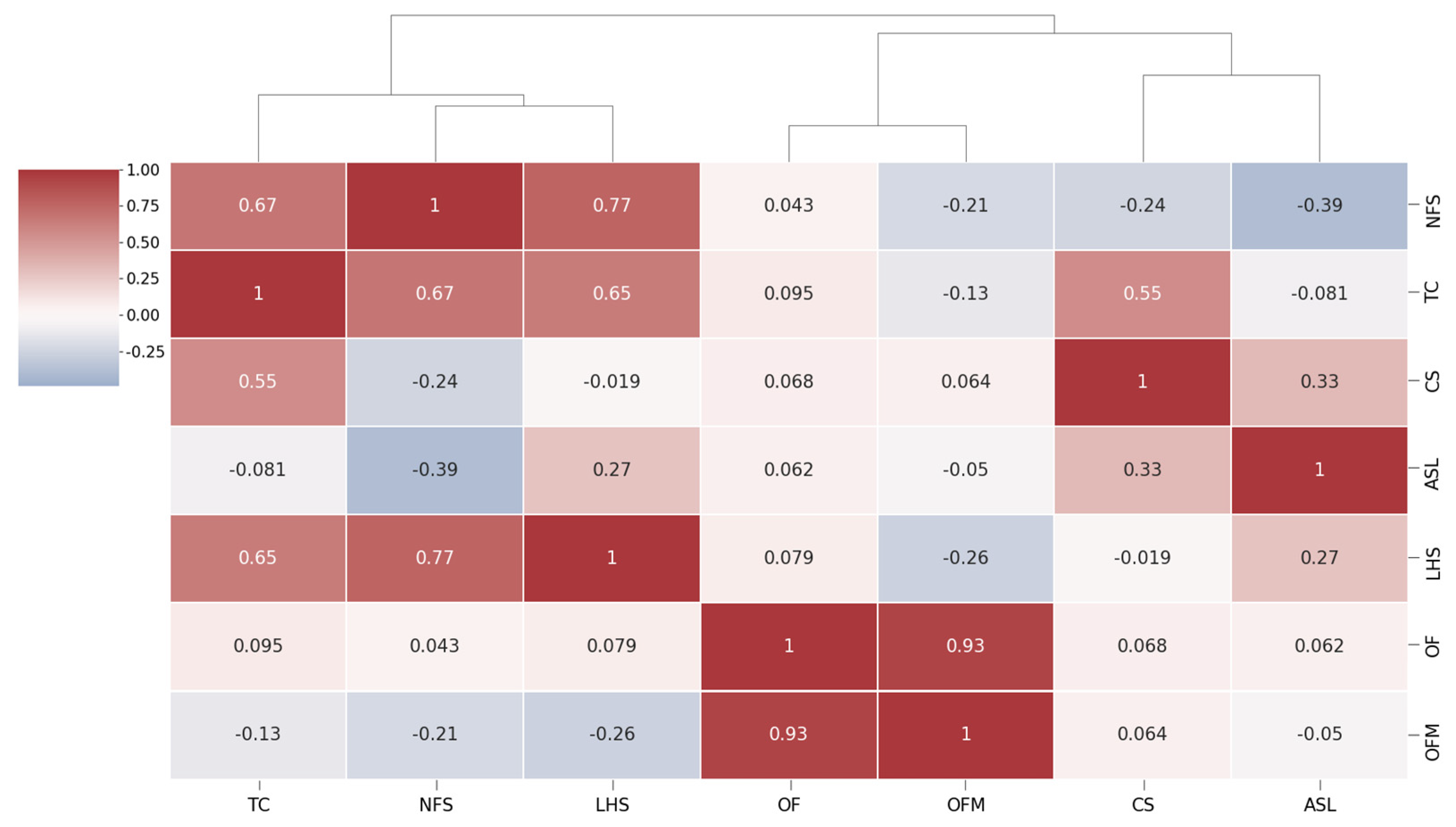
4.1. Process Design Correlation and Clustering Analysis Results

The method introduced in Section 3.4 was used to make a thermal clustering diagram for the horizontal well process design, as shown in Figure 2. From the correlation coefficients in Figure 2, we observe that the correlations of NFS, TC, CS, ASL, and LHS with OFC and OFCM in the horizontal well process design are very low, and some show negative correlations, indicating that the effective penetration rate of horizontal wells in the sweet spot area of the target formation system in the process design is very low, and the effective number of injection clusters is also very low, leading to the unsatisfactory volumetric modification of shale reservoirs.

From the clustering effect, the LHS, NFS, and TC with high correlation are divided into one big category; from the actual situation interpretation, we know that as LHS increases, NFS and TC will also increase. CS and ASL are combined into one category, which is easier to understand—because ASL increases, CS will also increase. In summary, the horizontal well process design clustering analysis is in line with the actual situation in the field, and the interpretation of the data is reasonable.

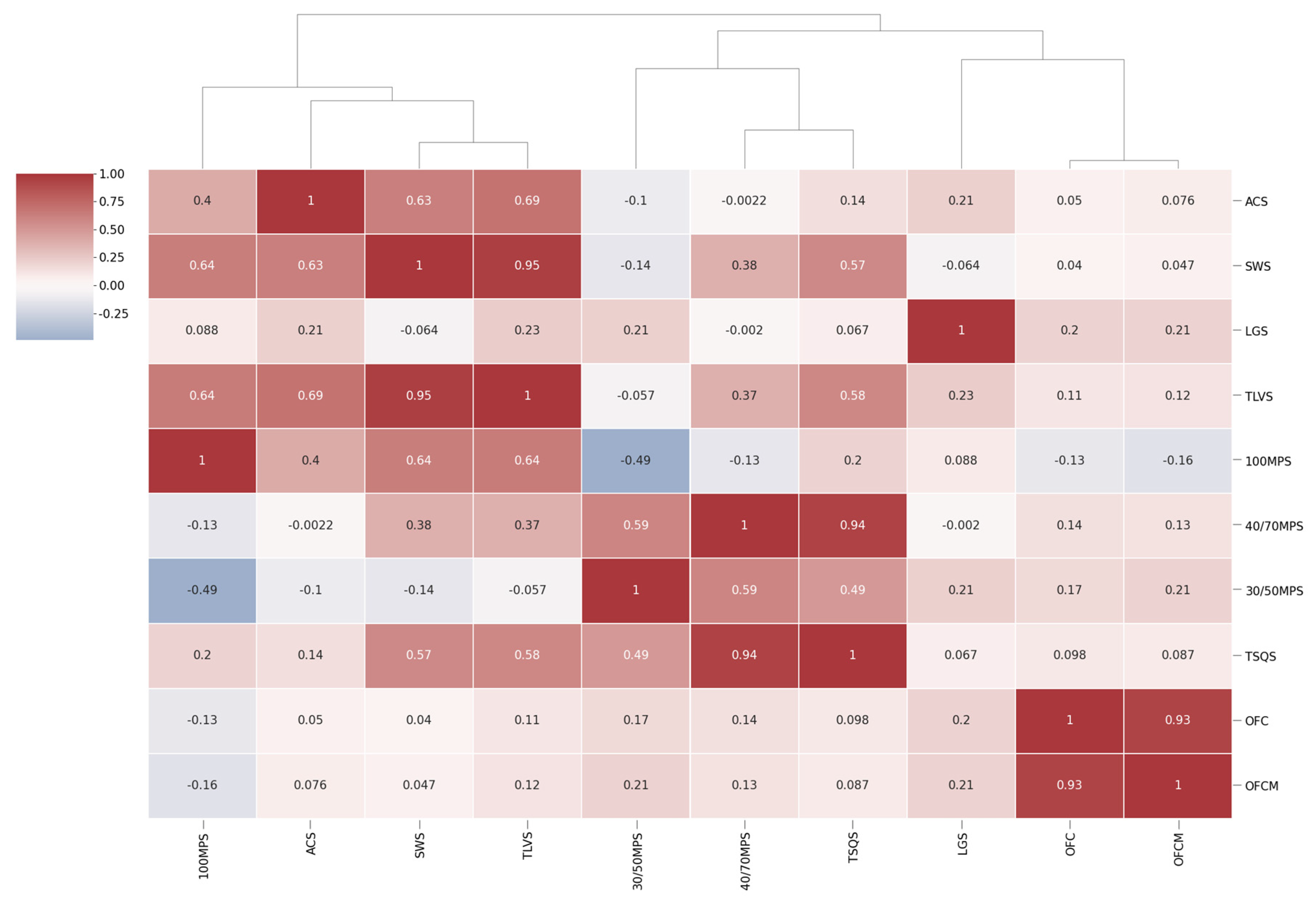
4.2. Correlation and Clustering Analysis Results of Fracturing Construction Parameters

Similarly, we produced a horizontal well fracturing construction thermal clustering diagram, as shown in Figure 3. From the correlation coefficients in Figure 3, the fracturing construction parameters correlate with the unimpeded flow rate per meter in high and low order (0.21, 0.21, 0.13, 0.12, 0.087, 0.076, 0.047, −0.13): LGS, 30/50 MPS, 40/70 MPS, TLVS, TSQS, ACS, SWS, 100 MPS. The 100 MPS shows a negative correlation with OFCM and a high linear correlation with TLVS and SWS, proving that it is too high to guide the Fuling area with the current construction design volume, and further analysis is needed to determine the appropriate construction interval.

The clustering analysis shows that 100 MPS is divided into a large category with ACS and SWS and TLVS, and not with TSQS, which verifies the previous idea that the 100 MPS design is not reasonable. All other parameters are in line with the actual field conditions of fracturing construction parameters. In the next study, the preferential selection of horizontal well process design parameters will not be further explored, as the analyzed reasonable parameters also mainly refer to the geological structure, sweet spot, and economic benefits in the actual field application. Among the fracturing construction parameters, considering their redundancy, TLVS and TSQS are excluded, and these two parameters are mainly the cumulative values of other parameters; therefore, the specific parameters analyzed are the following six: ACS, SWS, LGS, 100 MPS, 40/70 MPS, and 30/50 MPS.

4.3. Analysis of Fracturing Construction Parameters

According to the above summary analysis, the six parameters of fracturing construction are analyzed by the big data panel methods of scatter plot, violin plot, and binary kernel density estimation diagram (KDE). The general distribution range is observed according to the scatter plot, the distribution pattern and concentration range of construction parameters are obtained according to the violin plot, and the overall change trend is obtained according to the two-dimensional kernel density plot to further optimize the best parameter range for cost reduction and production increase. Here is an explanation of how KDE charts are preferential regions: KDE charts are actually a representation of probability density concentrations, similar to a two-dimensional histogram, where we can see the distribution of points from a scatter plot, but cannot tell the exact trend. However, the KDE plot allows you to visually see which direction the trend of the data set is likely to go, and thus the underlying pattern. This also leads to the concept of preferred regions, which is introduced next. (1) Stable concentration area—the area with the highest concentration of fracturing construction parameters for high-producing wells is delineated. (2) Risk-divided high-yield area—the area where the highest unimpeded flow rate per meter has occurred, or the area where the unimpeded flow rate per meter increases as the parameter value increases. (3) Cost reduction and efficiency area—the area where the unimpeded flow per meter remains the same or decreases slightly as the parameter value decreases. (4) Reducing cost and increasing production area—the area where the unimpeded flow per meter increases as the parameter value decreases.

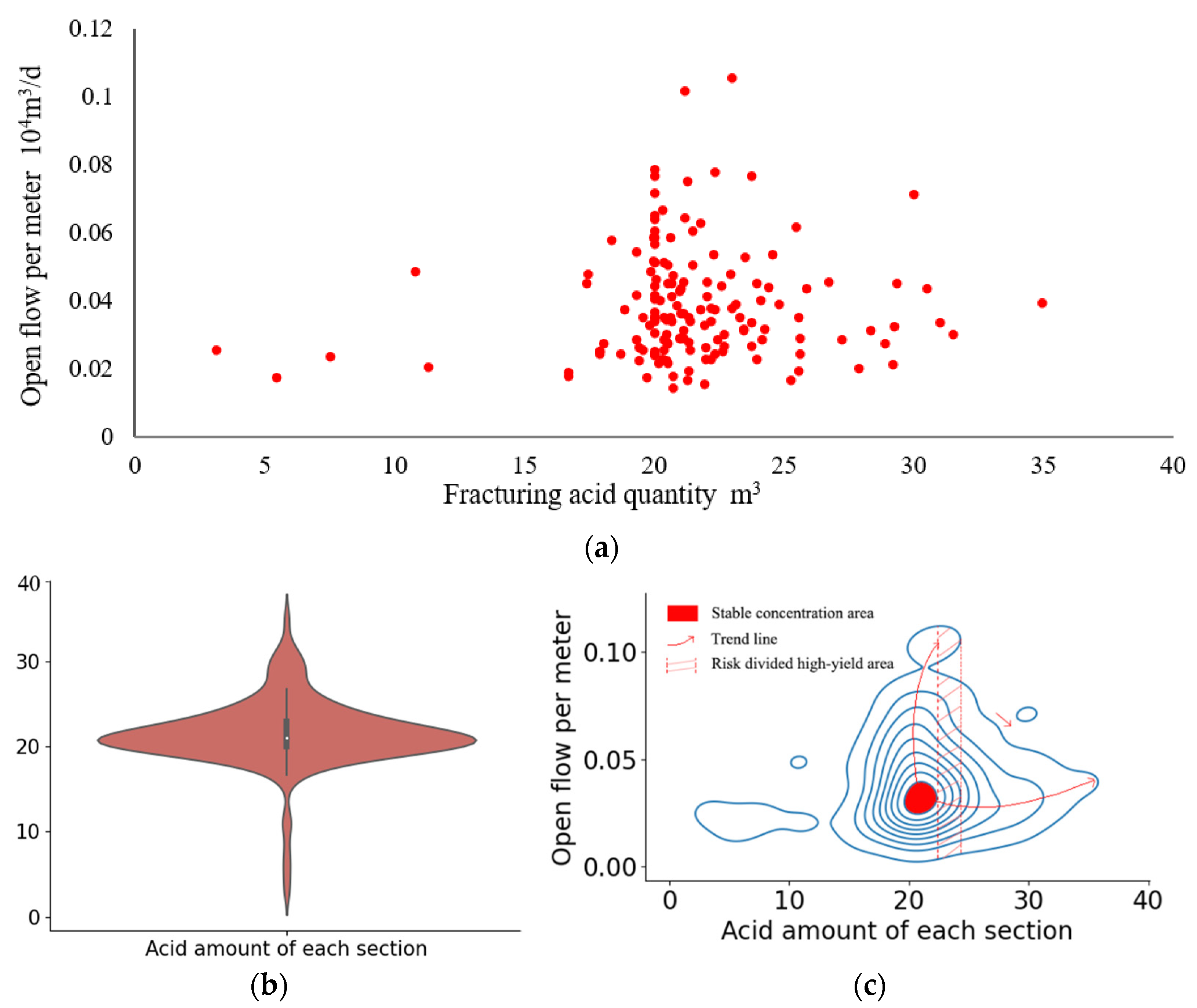
4.3.1. Optimization of Acid Amount in Each Section

The scatter diagram, violin diagram, and KDE are drawn according to the open flow per meter and acid amount in each section, as shown in Figure 4a–c. Figure 4a shows that the acid amount in each section of the high-yield wells is mainly about 20 m³. In Figure 4b, the median acid amount is 21 m³, the 95% data confidence interval is distributed between 16 and 26 m³, and the acid amount is concentrated in 21 m³. Figure 4c shows that the stable concentration area of high acid production wells in each section is mainly between 20 and 22 m³; however, from the trend line of the KDE, with the increase in acid amount, the overall trend is derived to the upper right. The highest OFCM appears at 24 m³. With the further increase in the acid amount, the OFCM gradually decreases. Therefore, combined with the change trend and the range of maximum OFCM, the risk-divided high-yield area of 22–24 m³ is obtained.

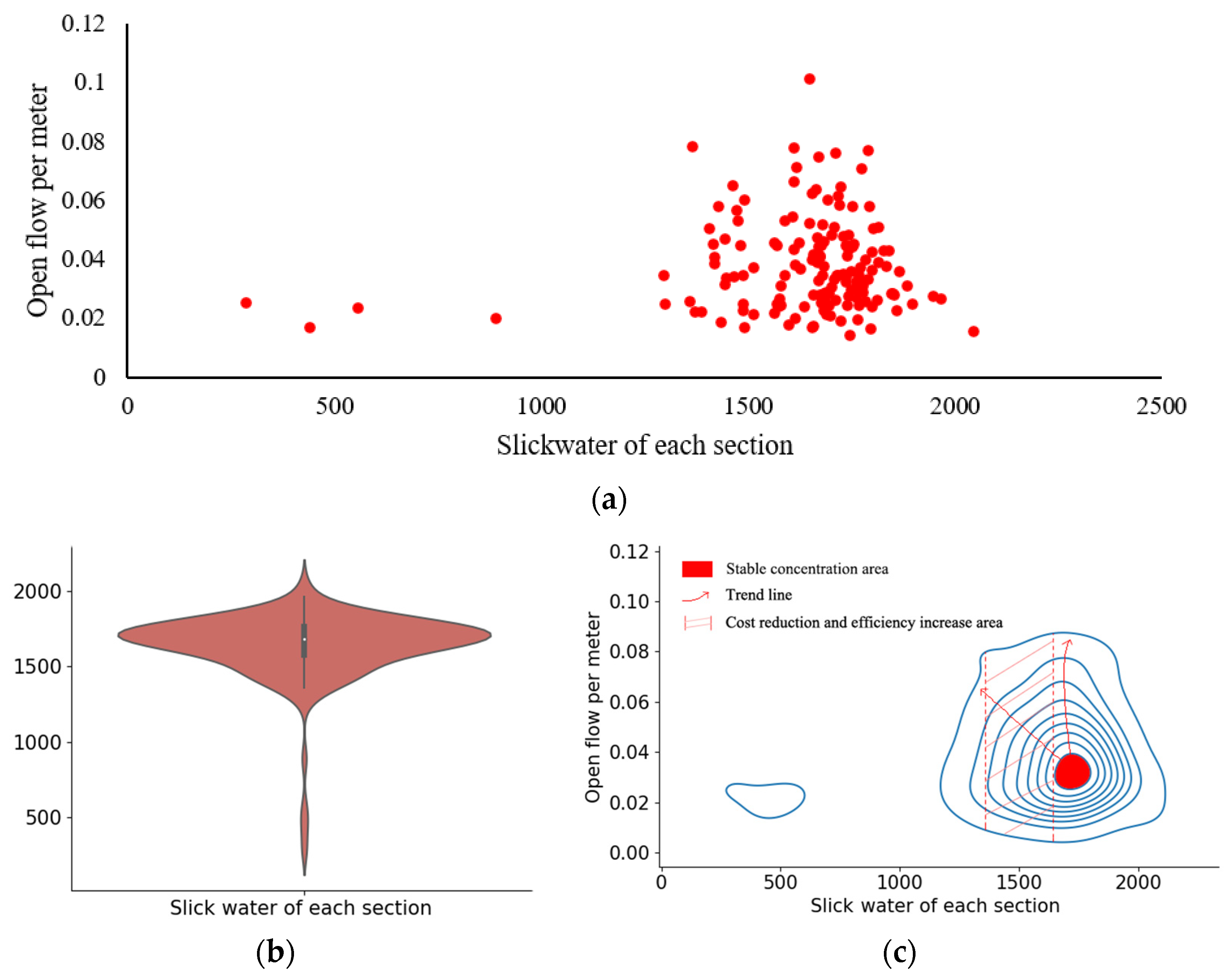
4.3.2. Optimization of Each Section of Slickwater

Similarly, the scatter, violin, and KDE diagrams of each section of slickwater are drawn as shown in Figure 5a–c, respectively. Figure 5a shows that each section of slickwater in the high-yield wells is mainly concentrated between 1300 and 1900 m³. Figure 5b depicts that the number of bits of slickwater in each section is 1680 m³, the 95% data confidence interval is distributed between 1380 and 1950 m³, and the slickwater is concentrated in 1700 m³. In Figure 5c, the stable concentration area of each section of acid production wells is mainly between 1660 and 1720 m³. From the stable concentration area to the right, with the increase in slickwater, the OFCM tends to decline slightly to the left, but the decline range is small; it decreases sharply from 1420 m³ to the left. Therefore, the cost reduction and efficiency area of 1420–1660 m³ can be obtained from the figure.

4.3.3. Linear Glue of Each Section

The linear glue, violin, and binary KDE diagrams of each section are drawn as shown in Figure 6a–c, respectively. Figure 6a shows that the linear glue of each section of the high-yield wells is evenly distributed, and there is no particularly concentrated area. In Figure 6b, we observe that the median linear gel is 145 m³, the 95% data confidence region is distributed between 0 and 350 m³, and the high-yield wells are concentrated around 150 m³. In Figure 6c, the stable concentration area of the high-yield wells is mainly between 85 and 160 m³. From the stable concentration area to the left, the OFCM decreases sharply with the decrease in linear glue. From the stable concentration area to the right, with the increase in linear glue, the OFCM shows an upward trend. After exceeding 250 m³, the OFCM decreases sharply. Therefore, the risk-divided high-yield area of 160–250 m³ is obtained.

4.3.4. 100 Mesh Proppant Per Section

The scatter, violin, and binary KDE diagrams of 100 mesh proppant in each section are drawn as shown in Figure 7a–c, respectively. In Figure 7a, we observe that the distribution of 100 mesh proppant in each section of the high-yield wells is relatively scattered, and there is no particularly concentrated area. Figure 7b shows that the median value of 100 mesh proppant in each section is 12.5 m³, the 95% data confidence interval is distributed between 2.5 and 22.5 m³, and the high yield is concentrated between 9 and 16 m³. Figure 7c indicates that the stable concentration area of the high-yield wells is mainly between 10.5 and 16 m³. From the stable concentration area to the left, with the decrease in 100 mesh proppant, the OFCM tends to increase and the highest yield appears between 7.5 and 10.5 m³. From the stable concentration area to the right, with the gradual increase in 100 mesh proppant, the OFCM rises slightly, but the overall trend is downward. Therefore, combined with the highest yield area and change trend, the reducing cost and increasing production area is 7.5–10.5 m³.

4.3.5. Proppant of 40/70 Mesh in Each Section

The scatter, violin, and binary KDE diagrams of 40/70 mesh proppant in each section are drawn as shown in Figure 8a–c, respectively. Figure 8a shows that the distribution of 40/70 mesh proppant in each section of the high-yield wells is mainly concentrated at 25–45 m³. In Figure 8b, the median value of 40/70 mesh proppant in each section is 36 m³, the 95% data confidence interval is distributed at 19–54 m³, and the distribution of the high-yield wells is concentrated at 35 m³. In Figure 8c, the stable concentration area of 40/70 mesh proppant in each section of the high-yield well is mainly between 32 and 38 m³. From the stable concentration area to the left, with the decrease in 40/70 mesh proppant, the OFCM decreases sharply. From the stable concentration area to the right, with the gradual increase in 40/70 mesh proppant, the OFCM is gentle, but shows a slight downward trend. Based on the above analysis, we concluded that the stable concentration area of 32–38 m³ is the best construction parameter range.

4.3.6. Proppant of 30/50 Mesh in Each Section

The scatter, violin, and binary KDE diagrams of 30/50 mesh proppant in each section are drawn as shown in Figure 9a–c, respectively. Figure 9a shows that the distribution of 30/50 mesh proppant in each section of the high-yield well is average and very scattered. In Figure 9b, the median value in each section is 1.8 m³, the 95% data confidence interval is distributed between 0 and 5 m³, and the high yield is concentrated between 0.5 and 2.2 m³. In Figure 9c, the stable concentration area of 30/50 mesh proppant in each section of the high-yield well is mainly between 0.4 and 1.8 m³. From the stable concentration area to the left, with the decrease in 30/50 mesh proppant, the OFCM decreases sharply. From the stable concentration area to the right, with the gradual increase of 30/50 mesh proppant, the OFCM decreases gently to 3.2 m³. Based on the above analysis, we concluded that the stable concentration area of 0.4–1.8 m³ is the best construction parameter range.

Through the above analyses, the stable concentration area of six main construction parameters of high-yield wells and the cost reduction and efficiency increase area, risk-divided high-yield area, and reducing cost and increasing production area of some parameters are obtained. The parameters of the stable concentration area are as follows: 20–22 m³ acid per section, 1660–1720 m³ of slickwater per section, 85–160 m³ of linear glue per section, 10.5–16 m³ of 100 mesh proppant per section, 32–38 m³ of 40/70 mesh proppant per section, and 0.4–1.8 m³ of 30/50 mesh proppant per section. The parameters of cost reduction and efficiency area are 1420–1660 m³ of slickwater in each section. The parameters of the risk-divided high-yield area are 22–24 m³ acid amount per section, and 160–250 m³ linear glue per section. The parameters of the reducing cost and increasing production area are 7.5–10.5 m³ of 100 mesh proppant per section, as shown in Figure 10.

5. Validation of Results

From the above analysis, four combinations can be obtained that are recommended for fracturing new wells: Type I—stable parameter range, Type II—production increase parameter range, Type III—cost reduction and production increase parameter range, and Type IV—highest production parameter range. Type I is the most concentrated and stable parameter range in high yielding wells. Type II is the parameter range with increased acid volume and linear rubber volume compared to Type I. Type Ⅲ is the parameter range in which the slickwater per section is reduced, and the 100 mesh proppant per section is reduced in comparison to Type Ⅰ. Type IV is the parameter range for maximizing production in comparison to Type I, regardless of the cost of fracturing construction parameters. The specific parameters are shown in

Table 5. Table of combinations of different parameter ranges.

	Type I (m3)	Type Ⅱ (m3)	Type Ⅲ (m3)	Type Ⅳ (m3)
Acid amount of each section	20–22	22–24	20–22	22–24
Slickwater of each section	1660–1720	1660–1720	1420–1660	1660–1720
Linear glue of each section	85–160	160–250	85–160	160–250
100 mesh proppant of each section	10.5–16	10.5–16	7.5–10.5	7.5–10.5
40–70 mesh proppant of each section	32–38	32–38	32–38	32–38
30–50 mesh proppant of each section	0.4–1.8	0.4–1.8	0.4–1.8	0.4–1.8

.

In order to verify the feasibility of the different parameter ranges, 12 wells with similar horizontal well process designs and fracture construction parameters belonging to Types I, II, III, and IV were identified from the analytical data, where a cost–benefit concept is the unimpeded flow rate generated per RMB, i.e., the ratio of the unimpeded flow rate to the cost of the fracture construction parameter usage, which provides a direct measure of the most productive combination for the same cost. See

Table 6. Evaluation of the effectiveness of horizontal wells under different fracturing construction combination modes.

	Open Flow Capacity (m3)	Fracturing Construction Materials Costs (¥)	Cost Benefit (m3/¥)	Average Open Flow Capacity (m3)	Average Cost Benefit (m3/¥)	Category
A1	453,000	3,013,520	0.1503	462,700	0.1480	I
A2	441,900	3,242,040	0.1363
A3	493,200	3,134,270	0.1573
A4	461,100	3,217,520	0.1433	471,200	0.1411	Ⅱ
A5	493,400	3,425,089	0.1441
A6	459,100	3,376,986	0.1359
A7	522,300	2,686,160	0.1944	481,767	0.1691	Ⅲ
A8	421,800	2,867,590	0.1470
A9	501,200	3,024,794	0.1656
A10	568,300	3,246,729	0.1750	526,733	0.1536	Ⅳ
A11	453,000	3,494,560	0.1296
A12	558,900	3,578,237	0.1562

Acid: 600 ¥/m³, slickwater: 60 ¥/m³, linear glue: 120 ¥/m³, 100 mesh proppant: 656 ¥/m³, 40–70 mesh proppant: 675 ¥/m³, 30–50 mesh proppant: 970 ¥/m³.

for details.

As can be seen in Table 6, the wells that have been fractured validate the preferred zones from our previous analysis. The highest to lowest yielding combinations are: Ⅳ, Ⅲ, Ⅱ, and Ⅰ. The best combinations in terms of economics are: Ⅲ, Ⅳ, Ⅰ, and Ⅱ. If the site is pursued for maximum production, Type IV fracturing is the best range of construction parameters, and if the extraction is done for economics, the Type III combination can be used.

6. Conclusions

This study is based on a big data analysis process, relying on fracturing data from 303 horizontal wells in the Fuling Shale Gas Demonstration Area to explore some of the columns. The paper applies Pearson and UPGMA methods to the correlation clustering analysis of horizontal well fracturing design parameters and fracturing construction parameters. The big data panel method was applied to specific fracturing construction parameters to determine different preferred zones and give ways to combine different zones. New ideas for the design of fracturing schemes are provided for engineers working in the front line.

As this study focuses on the Fuling shale gas demonstration area in China, the conditions for data preprocessing are changed for the analysis of other oil and gas reservoirs (Section 3.2). As the Fuling shale gas block is an emerging one in China, the volume of accumulated data is not very large. Therefore, subsequent studies can collect as many parameters as possible, such as quantitative characterization of the fracture complexity of each well, quantitative characterization of the post-pressure G function, and use the cumulative gas production as a criterion for high or low production, which can lead to richer results.

References

1. Ping, Y.Q.; Sheng, F.L.; Zhou, N.; Li, P.; Lv, J. Analysis of the Application of Big Data Technology in Oil and Gas Geological Exploration. Sci. Technol. Inf. 2019, 17, 59–60. [Google Scholar]
2. Yang, C.S.; Zhang, H.L. An Introduction to the Application and Challenges of Big Data in the Domestic Oil Exploration and Development Industry. Sci. Inform. 2019, 20, 19–20. [Google Scholar]
3. Tian, J.H.; Zhang, B. The Practice and Prospect of Big Data Technology in Petrochemical Industry; Sinopec Publishing House: Beijing, China, 2016. [Google Scholar]
4. Hailin, S.; Peng, Z.; Xiaotao, Y.; Kebin, X.; Qing, C.; Qi, Z. Parameter Design Method for Re-Fracturing Scheme of Water Injection Block in Oil and Gas Field. Well Test 2020, 29, 6–13. [Google Scholar]
5. Dou, X.; Liao, X.; Hou, T.; Zhao, T.; Zhiming, C.; Ren, W.; Zhang, R. Fracture Optimization for Multi-Stage Fractured Horizontal Well with Time & Stress-Sensitive Parameters. In Proceedings of the Nigeria Annual International Conference and Exhibition, Lagos, Nigeria, 2 August 2015. [Google Scholar] [CrossRef]
6. Feng, Q.; Liu, J.; Huang, Z.; Tian, M. Study on the Optimization of Fracturing Parameters and Interpretation of CBM Fractured Wells. J. Nat. Gas Geosci. 2018, 3, 109–117. [Google Scholar] [CrossRef]
7. Yao, J.; Li, Z.; Liu, L.; Fan, W.; Zhang, M.; Zhang, K. Optimization of Fracturing Parameters by Modified Variable-Length Particle-Swarm Optimization in Shale-Gas Reservoir. SPE J. 2021, 26, 1032–1049. [Google Scholar] [CrossRef]
8. Fan, Y.L. Optimization of Hydraulic Fracturing Treatment Parameters for Tight Gas Reservoirs Using Machine Learning. Ph.D. Thesis, Xi’an Shiyou University, Xi’an, China, 2021. [Google Scholar]
9. Tang, C.; Chen, X.; Du, Z.; Yue, P.; Wei, J. Numerical Simulation Study on Seepage Theory of a Multi-Section Fractured Horizontal Well in Shale Gas Reservoirs Based on Multi-Scale Flow Mechanisms. Energies 2018, 11, 2329. [Google Scholar] [CrossRef] [Green Version]
10. Xu, B.; Liu, Y.; Wang, Y.; Yang, G.; Yu, Q.; Wang, F. A New Method and Application of Full 3D Numerical Simulation for Hydraulic Fracturing Horizontal Fracture. Energies 2019, 12, 48. [Google Scholar] [CrossRef] [Green Version]
11. Yan, X.Z.; Lei, J.J.; Ren, J. Optimization of Volumetric Fracturing Parameters for Tight Oil Reservoirs in Southern Exploration Area. Unconv. Oil Gas 2020, 7, 113–120. [Google Scholar]
12. Wang, J.; Sun, J.; Liu, D.; Zhu, X. Production Capacity Evaluation of Horizontal Shale Gas Wells in Fuling District. FDMP Fluid Dyn. Mater. Process. 2019, 15, 613–625. [Google Scholar] [CrossRef]
13. Liu, M.J.; Wang, X.F.; Huang, Y. Data Preprocessing in Data Mining. Comput. Sci. 2000, 27, 56–59. [Google Scholar]
14. Kan, Z.G.; Jin, X. Research and Implementation of Data Preprocessing in Data Mining. Comput. Appl. Res. 2004, 07, 118–119. [Google Scholar]
15. Pearson, K. Notes on Regression and Inheritance in the Case of Two Parents. Proc. R. Soc. Lond. 1895, 58, 240–242. [Google Scholar]
16. Myers, J.L.; Well, A.D. Research Design and Statistical Analysis, 2nd ed.; Lawrence Erlbaum: Mahwah, NJ, USA, 2003. [Google Scholar]
17. Wang, X. Nonparametric Statistics; Renmin University of China Press: Beijing, China, 2005. [Google Scholar]
18. Gronau, I.; Moran, S. Optimal Implementations of UPGMA and Other Common Clustering Algorithms. Inf. Process. Lett. 2007, 104, 205–210. [Google Scholar] [CrossRef]
Figure 1. Fuling phase I production and construction area.
Energies 14 08357 g001
Figure 2. Thermal clustering diagram of horizontal well process design parameters.
Energies 14 08357 g002
Figure 3. Thermal clustering diagram of horizontal well fracturing construction parameters.
Energies 14 08357 g003
Figure 4. Analysis of acid quantity data. (a) Scatter plot of acid content; (b) violin plot of acid content; (c) binary KDE plot of acid quantity.
Energies 14 08357 g004
Figure 5. Analysis of slickwater data. (a) Scatter plot of slickwater; (b) violin plot of slickwater; (c) binary KDE plot of slickwater.
Energies 14 08357 g005
Figure 6. Analysis of linear glue data. (a) Scatter plot of linear glue; (b) violin plot of linear glue; (c) binary KDE plot of linear glue.
Energies 14 08357 g006
Figure 7. Analysis of 100 mesh proppant data. (a) Scatter plot of 100 mesh proppant; (b) violin plot of 100 mesh proppant; (c) binary KDE plot of 100 mesh proppant.
Energies 14 08357 g007
Figure 8. Analysis of 40/70 mesh proppant data. (a) Scatter plot of 40/70 mesh proppant; (b) violin plot of 40/70 mesh proppant; (c) binary KDE plot of 40/70 mesh proppant.
Energies 14 08357 g008aEnergies 14 08357 g008b
Figure 9. Analysis of 30/50 mesh proppant data. (a) Scatter plot of 30/50 mesh proppant; (b) violin plot of 30/50 mesh; (c) binary KDE plot of 30/50 mesh proppant.
Energies 14 08357 g009
Figure 10. Optimal area range of fracturing construction parameters.
Energies 14 08357 g010