Application of Electrical Tomography Imaging Using Machine Learning Methods for the Monitoring of Flood Embankments Leaks

Abstract

This paper presents an application for the monitoring of leaks in flood embankments by reconstructing images in electrical tomography using logistic regression machine learning methods with elastic net regularisation, PCA and wave preprocessing. The main advantage of this solution is to obtain a more accurate spatial conductivity distribution inside the studied object. The described method assumes a learning system consisting of multiple equations working in parallel, where each equation creates a single point in the output image. This enables the efficient reconstruction of spatial images. The research focused on preparing, developing, and comparing algorithms and models for data analysis and reconstruction using a proprietary electrical tomography solution. A reliable measurement solution with sensors and machine learning methods makes it possible to analyse damage and leaks, leading to effective information and the eventual prevention of risks. The applied methods enable the improved resolution of the reconstructed images and the possibility to obtain them in real-time, which is their distinguishing feature compared to other methods. The use of electrical tomography in combination with specific methods for image reconstruction allows for an accurate spatial assessment of leaks and damage to dikes.

1. Introduction

Floods cause enormous damage, and are the cause of many tragedies. Therefore, the monitoring of flood defences is important for the safety of people and the environment. However, the methods used to identify cracks and seepage in dikes visually are insufficient. A dedicated monitoring system should be able to test dikes for seepage.

There are several methods which are used to analyze flood embankments.

Table 1. Main advantages and disadvantages of the different methods used in the study of dikes.

	Advantages	Disadvantages
Point measurements	Simple solution. Low costs. Constant monitoring.	No spatial analysis of the study site. Invasive.
Thermography	Ability to quickly analyze the external shaft. Low cost. Non-invasive.	No information on damage, internal seepage. Unit measurements.
Geophysical methods	Large area analysis/ Non-invasive.	Low efficiency in testing for leakage and shaft saturation.
Ground penetrating radar	Quick and easy measurements. Low costs. Non-invasive.	Proper development of radarograms is very complicated.
Optical methods	Ability to analyze the dike along its course. Continuous monitoring.	No information on area changes.
Electrical Resistance Tomography device	Ability to analyze 2D/3D parts of the shaft with the ERT device. Non-invasive.	Using only built-in measurement and reconstruction methods. Unit measurements.
Distributed electrical impedance tomography system	Area ability analyze any portion of the levee or all of it through a distributed cyber-physical system. Continuous monitoring. Non-invasive.	High costs.

shows the main advantages and disadvantages of each method. Geophysical methods are used in environmental studies to image objects [1]. They are characterized by their non-invasive character and the possibility of rapid imaging in soil. The GPR radar method is based on the waves passing through the object and allowing the analysis of their propagation through the analysis of the reflected signal, by which changes in the structure of the investigated medium can be observed [2]. Another method is thermography, which uses the phenomenon of the non-contact detection of electromagnetic radiation in the mid-infrared band. By analizing thermal images at different time intervals, changes in flood weights can be detected [3]. Another type of method is based on the analysis of the propagation of the generated electric current in the studied medium. This solution determines changes in the physical parameters of the tested object (resistivity). Finally, electrical resistivity tomography (ERT) [4,5,6] is used to study shafts. The resistivity tomography method consists of placing the measuring electrodes along the profile line at equal distances. Resistivity tomography is a technique which is often used for the imaging of geological soil properties. The electrical properties of soil are strongly influenced by such hydrological properties of rocks and soils as porosity and water saturation. Diffuse optical sensing [7,8,9,10,11,12], where optical fibres are placed at the bottom of the embankment, is also used for the monitoring of dikes. This use of sensors allows the reconstruction of temperature and strain profiles. However, it should be noted that distinguishing seepage in the obtained temperature data from terrain anomalies within earth embankments is still a difficult task. It should also be mentioned that fibre optic sensors require physical contact with the seepage material. Therefore, proper installation can become an invasive and challenging issue, especially when using this technology to monitor existing levees. However, fibre optics can be a very efficient and cost-effective solution for the monitoring of long stretches of new embankments where fibre optics can be easily installed within the embankment.

The Electrical Impedance Tomography (EIT) method enables the analysis of cracks and seepage [13] by taking measurements reconstructing them appropriately in the form of an image [14,15,16,17]. The monitoring of dikes, levees, dams, and floodwalls is a key process affecting the maintenance and reliability of these structures due to catastrophic effects and high possible damage costs [18]. The continuous and multi-level control of the technical condition of embankments is costly. Therefore, there is a great need to replace traditional observation methods with cyber-physical systems, in which impedance tomography (EIT) plays a key role [18,19,20,21]. The disadvantage of the commonly used solutions is the point measurement [22]. The most common cause of damage to shafts is water that penetrates through seepage and leaks. With the EIT implemented in cyber-physical monitoring systems, it is possible to obtain a cross-sectional view of the dike interior [23,24]. The image quality and resolution are sufficient to detect water-penetrated areas [25]. Early information about hazards helps to prevent severe damage. Despite significant advances in dike design and construction, unexpected events may occur. Therefore, designing an economical and reliable device to monitor the condition of dikes or flood-control reservoirs is crucial to prevent the devastating effects of flooding.

In tomographic systems, the image quality and its parameters—model geometry, spatial resolution, number of sensors, discretization, and reconstruction method—are important factors. Different deterministic and machine learning methods are used to solve inverse problems depending on the tomographic technique used. The goal of these methods is to obtain the expected solution quickly and with a good image reconstruction quality. Electrical impedance tomography has a relatively low image resolution. However, in the developed methods, the resolution is sufficient for seepage analysis or shaft condition monitoring.

The motivation for the research was to develop a distributed system to analyze dikes by spatially analyzing their condition in real-time. The main objective was to develop a comprehensive solution consisting of a measurement device, measurement electrodes, algorithms to reconstruct images from measurement data, and a cyber-physical system to monitor the dike condition. The solution based on electrical impedance tomography was chosen because of the possibility of the area analysis of the tested object using measurements on the near-surface of the tested object, the method of data acquisition, and the possibility of the analysis of changes in the values of electrical parameters. Besides this, electrical impedance tomography is quite sensitive to cracks and seepage, which undoubtedly makes it effective in shaft monitoring.

The authors’ main contribution is the development of a solution based on machine learning algorithms that work individually for each pixel of a tomographic image. The primary goal was to increase the resolution of the image reconstruction an-d enhance the system’s ability to identify different kinds of anomalies within flood embankments. The system architecture is shown in Figure 1. The data are collected from the tomographic equipment and then sent to the analysis software system.

The subject of the application of logistic regression with an elastic net regularisation [26], principal components analysis (PCA) [27] and wavelet preprocessing [28] in electrical impedance tomography [29,30] has been undertaken to verify and test the extent to which this approach can be helpful in the study of EIT dikes. For this purpose, numerical models and real models with different variations of electrode placement were prepared. Furthermore, the measurements from the tomograph were used to reconstruct the image of the object’s interior by collecting and analysing the data using machine learning methods.

The paper is divided into five sections, with an introduction. The architecture of the designed system is presented in Section 2. It also describes the measurement device, laboratory measurements, numerical models and machine learning algorithms. The work results obtained by reconstructing the corresponding images for the synthetic and measurement data are presented in Section 3. Section 4 discusses the results obtained, while Section 5 summarises the research carried out.

2. Materials and Methods

The following section presents electrical tomography’s structure and measurements, elements, apparatus, image reconstruction models from simulated and real measurements, and mathematical algorithms. In addition, the data collection methods and measurement methods are presented. The data are used in the next step to solve progressive and inverse problems. In the following subsections, several algorithms that were used in this work are described. These are wavelet-preprocessing, elastic net, and PCA algorithms. The above algorithms were used for tomographic imaging, and finally, they were compared. The above methods were used to obtain rapid and efficient solutions to build models on the reconstructed areas. The work was performed using tomographic equipment designed and manufactured at Netrix SA Research and Development Center. Additionally, Matlab, Python in R language and Eidors packages and tools were used [31].

2.1. Electrical Tomography

Electrical impedance tomography [32,33], generally called electrical tomography (ET) [34,35], includes some image reconstruction techniques. The methods available in the literature are electrical resistance tomography (ERT) [36,37], electrical capacitance tomography (ECT) [38,39,40,41] and electrical impedance tomography. ECT is based on the reconstruction of the electrical permeability ε, whereas EIT is based on the reconstruction of the conductivity γ. It is worth noting that electrical tomography has a low image resolution. This is caused by the limited number of current flow measurements through the test piece and the low sensitivity of the measured voltages, which depends on the conductivity change inside the test piece. In EIT, the current or voltage is introduced into an object through a set of sensors attached to its surface. The voltage drop values are measured on the other sensors. The properties of the test object are reconstructed by solving the inverse problem. Using the electrical properties of the materials, the interior of the test object can be mapped. Impedance tomography uses the conductivity of objects; by connecting a current or voltage source, a current flow or voltage distribution is forced. The current or voltage is observed to flow at the edge of the test area. The data collected in this way are used to build images using reconstruction algorithms. The image thus prepared is called a tomogram.

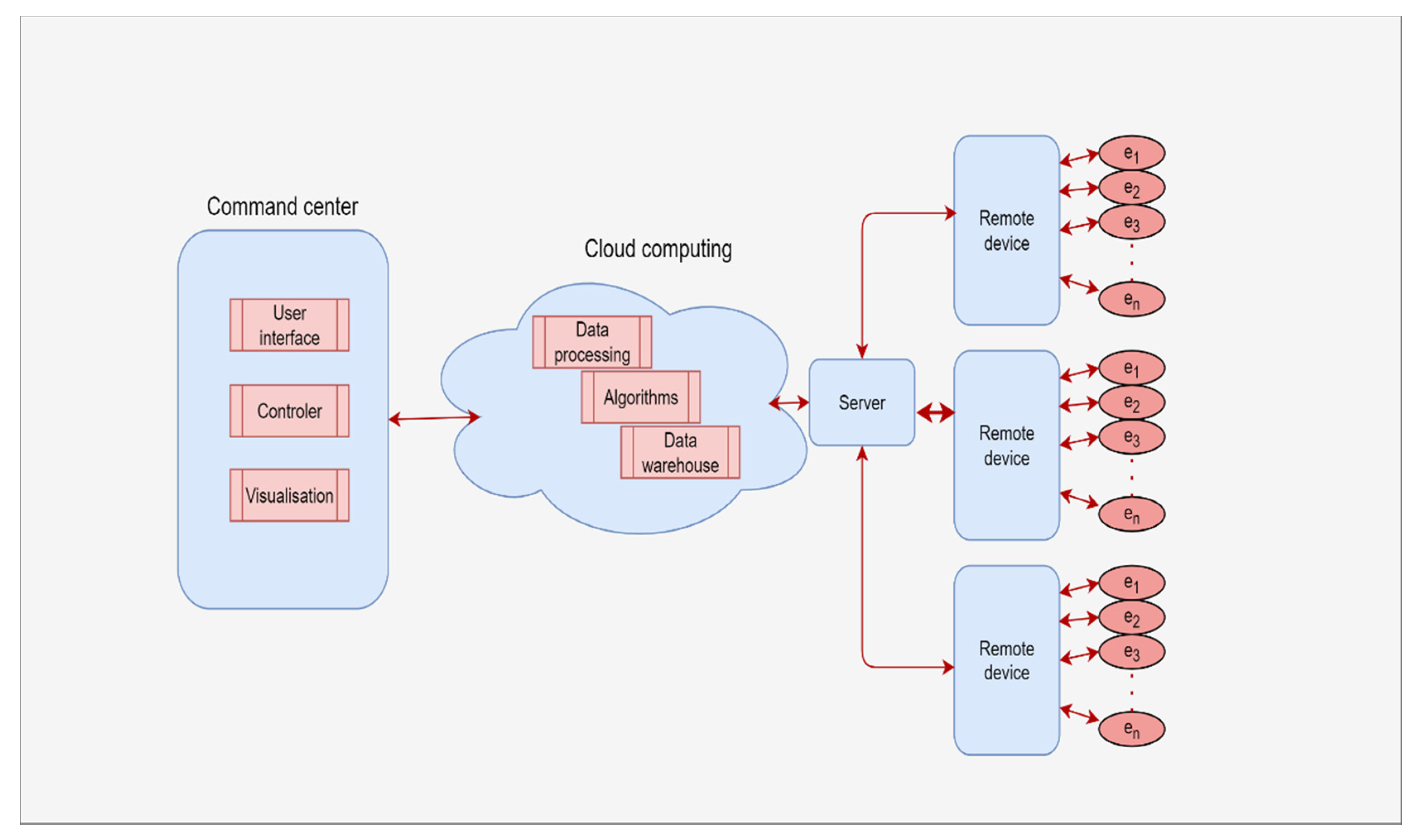
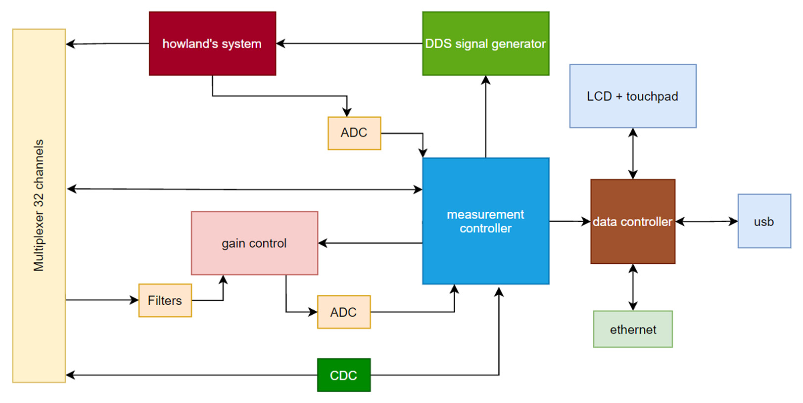
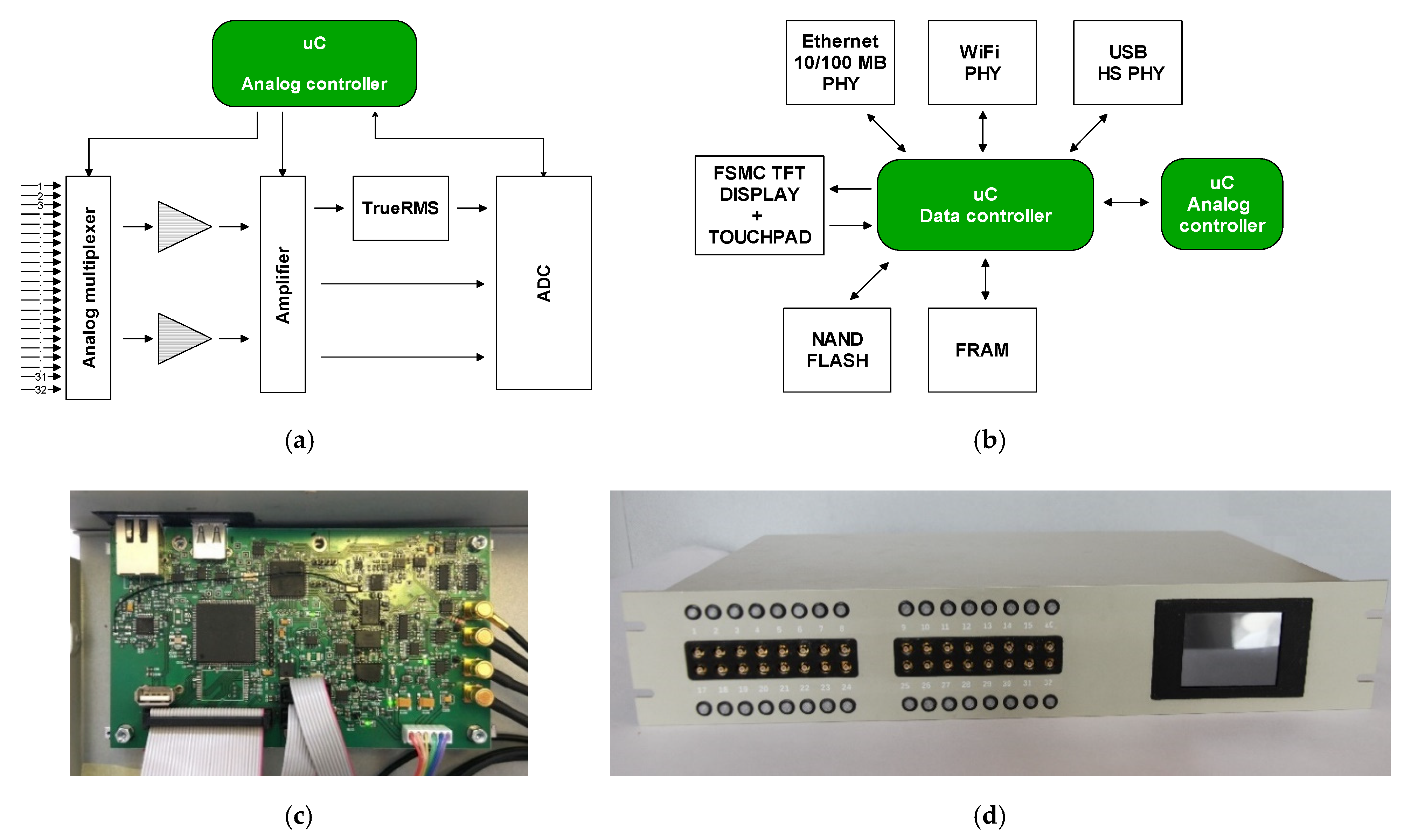
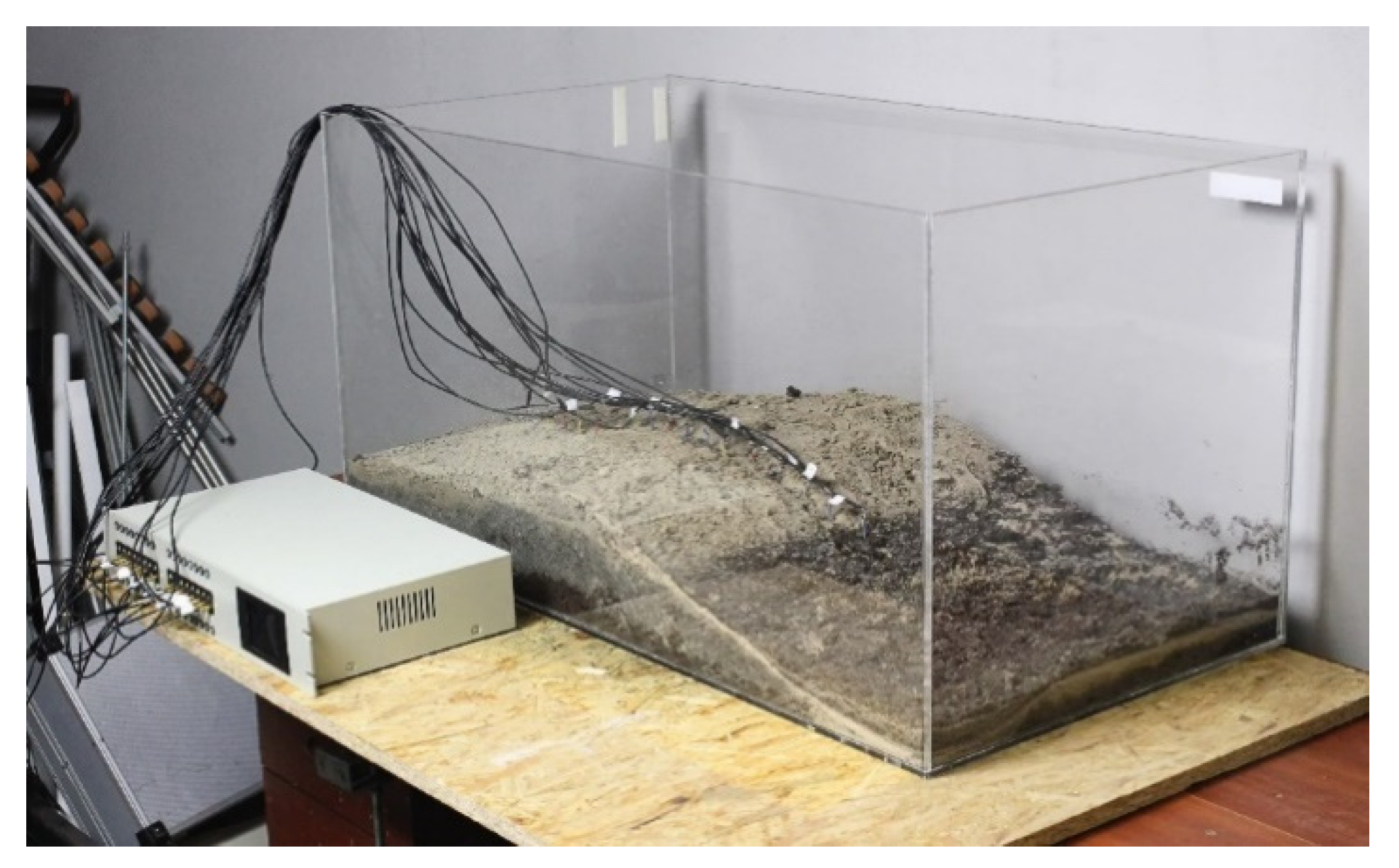
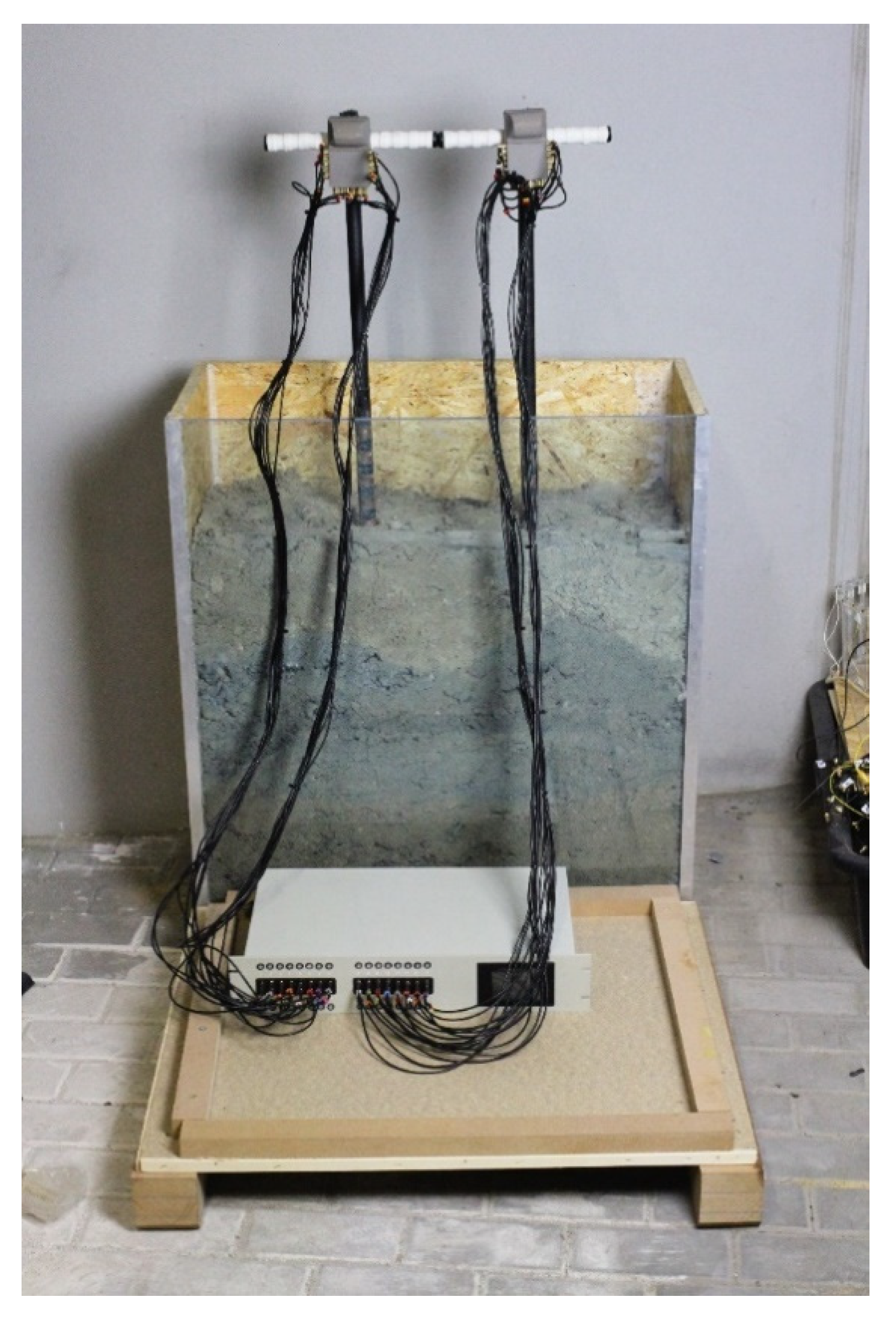
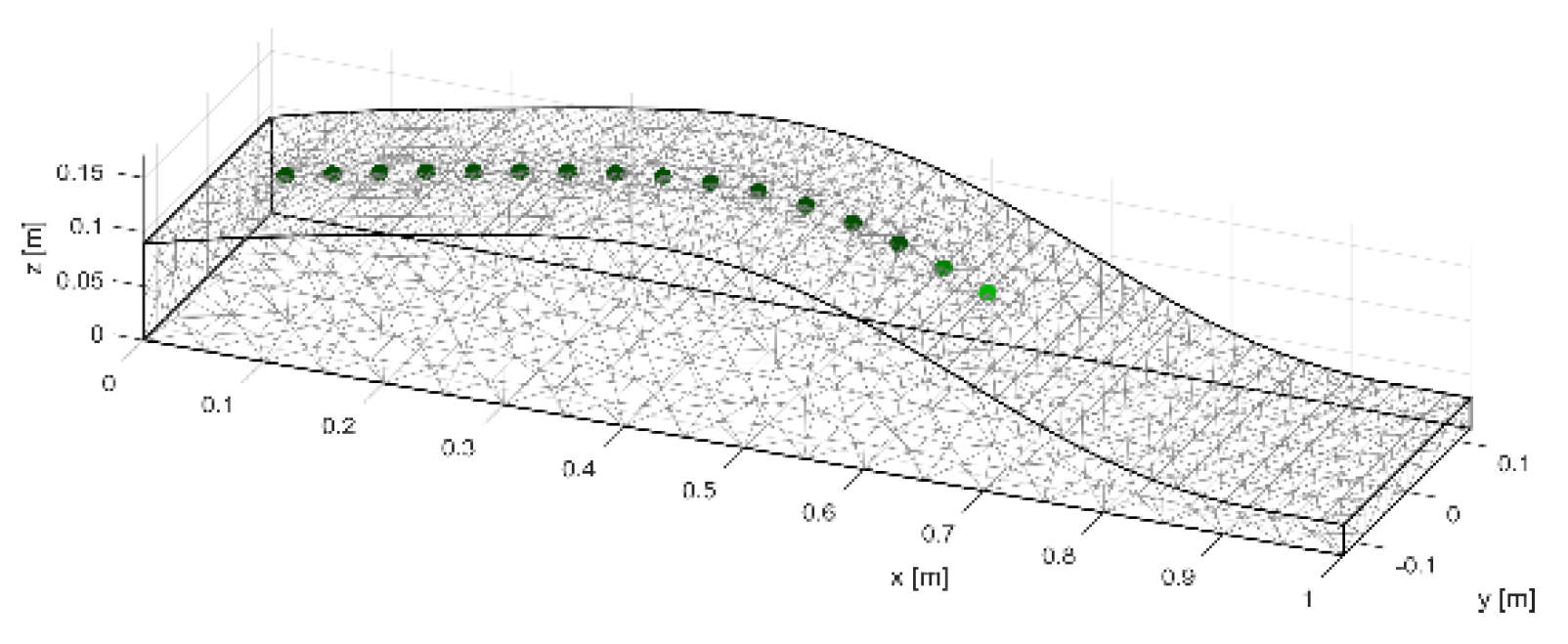
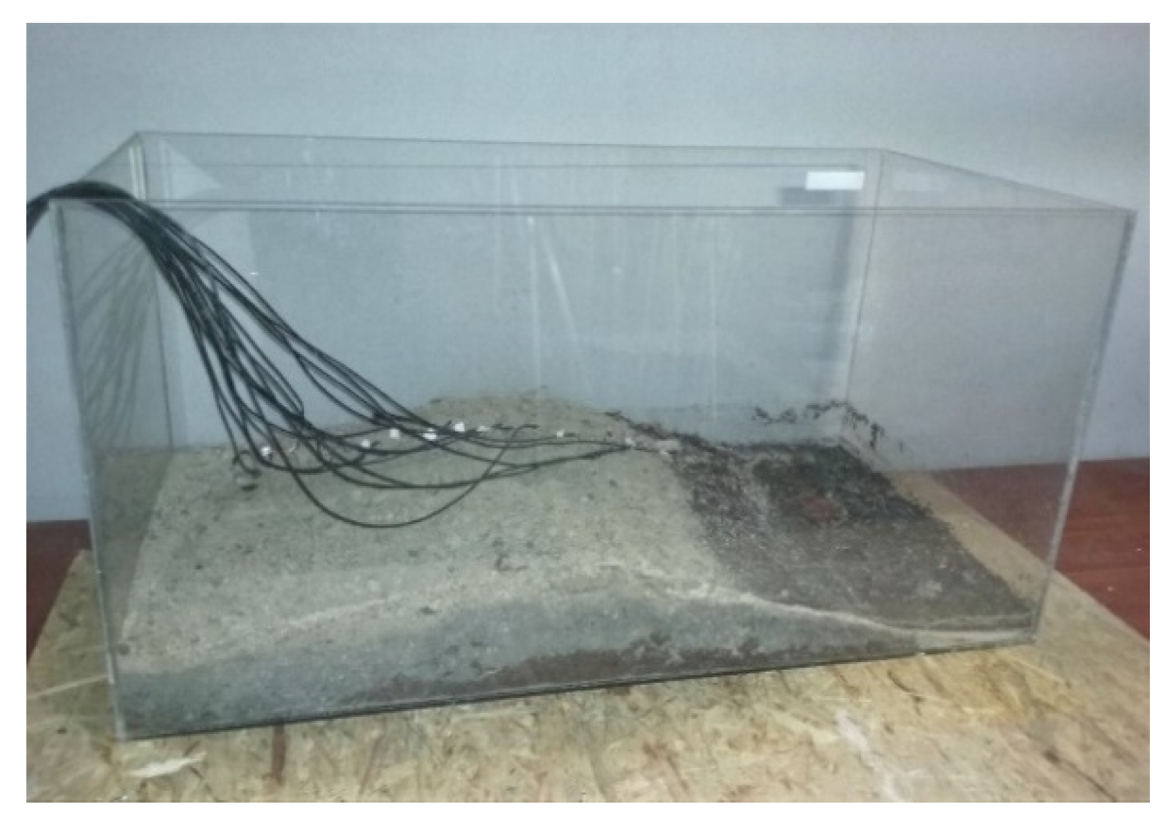
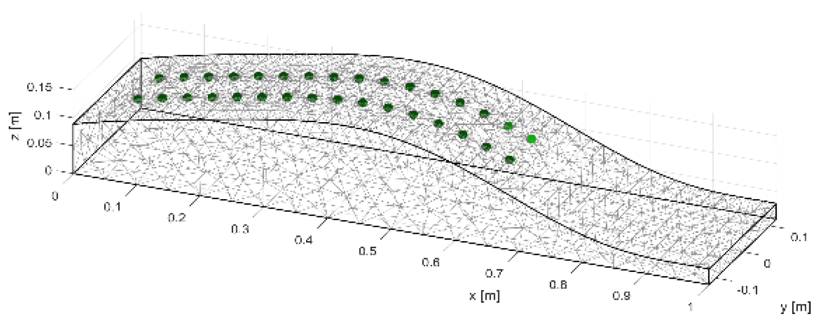
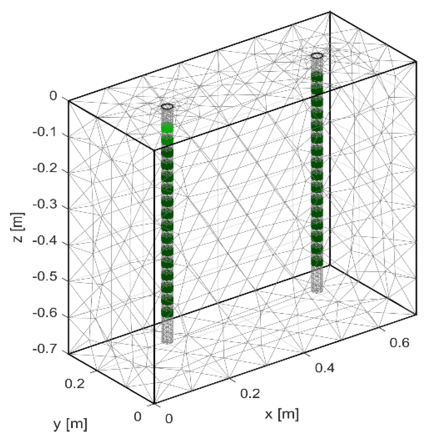
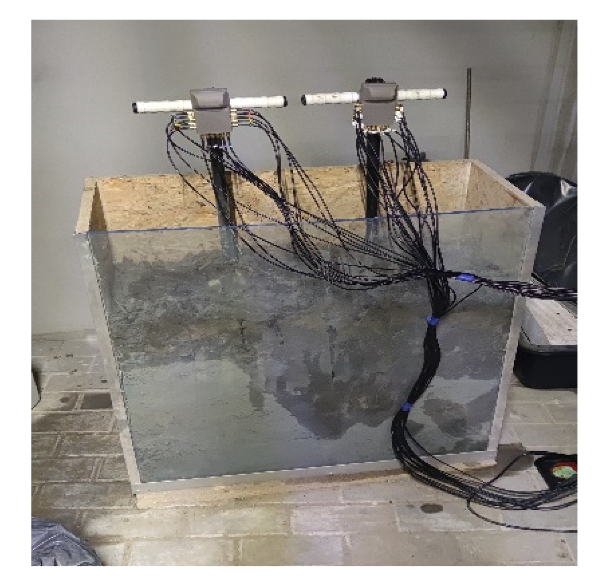
2.2. Measurement System

The system collects measurement data from the electrodes through a tomographic device that allows the measurement of up to 32 channels. The entire infrastructure is centrally managed for data collection and measurement recording. The application enables measurement collection, data management and device monitoring.

A finite element model and a real measurement model were prepared to test the effectiveness of different algorithms for the analysis of the procedures in tomography. In turn, electrical impedance tomography was used for the analysis.

The measurements were performed with a hybrid tomograph that bases its data controller and measurement structure on two stm32 controllers from the F4 family. Thanks to this solution, the measuring processor does not generate complex graphical interfaces; rather, it only performs the necessary operations in the tomographic process. This further significantly improves the solution performance. Figure 2 shows the block diagram of the built tomograph. The device is shown in Figure 3 as measurement block, a control and communication system, an inside view, and a measurement panel.

The excitation signal source was built on a direct digital synthesis (DDS) signal generator coupled with a current-generation system. The signal prepared in this way is then sent to the inputs of the multiplexer system, where—depending on the sequence of current measurements—it is transmitted to the selected output. The measurement controller performs the control of the currently measured/selected item. The measuring block consists of a set of active filters minimising the influence of the 50 Hz components on the measurement accuracy. The prepared signal travels to the digitally controlled gain control system, and to the Analog-to-Digital Converter (ADC). Each correct measurement of the matrix is sent to the control system, which, depending on the selected configuration, performs the process of recording or sending data to the server. Thanks to the integrated measuring circuit (capacitance/impedance), the device can be used to perform both EIT (impedance) and ECT (capacitance) measurements. The device is designed to work with sets of 8, 16 and 32 electrodes. The measurement takes place sequentially, depending on the selected mode. Two modes of EIT measurement are available (polar Ground GND—measurement against the negative electrode; polar NB—differential measurement). In the case of ECT measurements, only one mode is available: interelectrode measurement. In addition to mode selection, the instrument allows the user to choose the results’ averaging level and select the gain parameters. A 2.4-inch graphic touch screen is used to operate the instrument, select the functions and start the measurement process. The instrument enables the storage of the data on a portable memory carrier (pen drive), and allows the user to stream it via a serial port or the Ethernet.

The experiments were conducted on two measurement models. The first model (Figure 4) uses an array of 16 measurement electrodes equally spaced along the profile line, and a measurement array with 32 electrodes evenly spaced in two rows. In contrast, the second model consists of two multi-sensor arrays with 32 measuring electrodes (Figure 5). The EIT’s task is to generate an electrical current with specific parameters for each pair of sensors, read the voltage between each electrode, and send the data to the output. The flood embankment models were designed to represent the key parameters of the existing facility as accurately as possible.

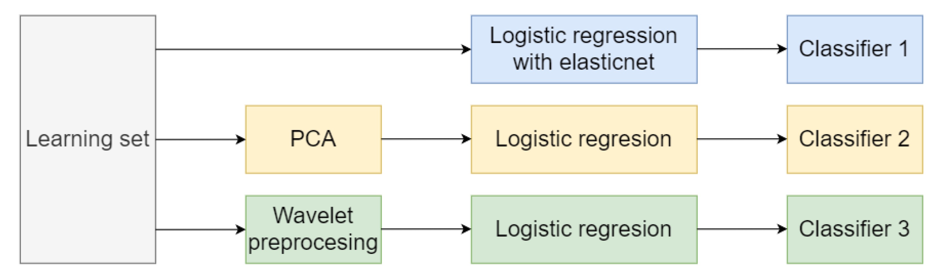
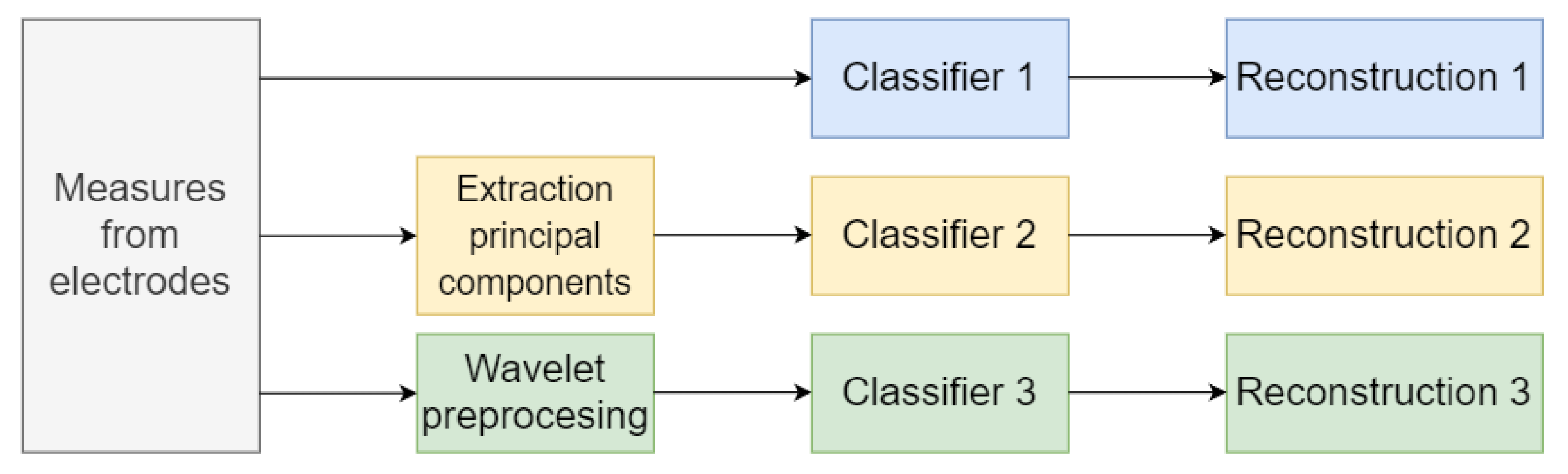
2.3. Algorithms and Methods

Many deterministic, statistical, or computational intelligence methods solve optimisation tasks [42,43,44,45]. In this paper, the authors concentrate on the use of machine learning. In addition to the real models, the imaging domain had to be prepared as a composite finite-element mesh model. In this case, a model was created for each element, representing the relationship between the value of the signal coming from the electrodes and the conductivity. If a different conductivity comes out of the measurements than that in the background measurements, there is a water concentration in the area. With the above information and measured values, the location of the flooded embankment can be determined. Therefore, a model is defined for each finite element. This allows the calculation of the probability of conductivity that differs from the background conductivity for each finite element. Based on this, the resolution in the imaging domain was determined, and thus, the mesh was reconstructed. The resolution of the imaging domain closely depends on the classification level, and it is the classification level that determines the occurrence of conductivity which is different from the background conductivity. By performing ROC analysis [46,47], each finite element’s classification level was determined, which should be understood here as the limiting probability of percolating conductivity.

2.3.1. Logistic Regression

Knowing the model and the background measurement, we need to answer the question of which finite elements in the area belong to the background and which belong to the inclusions. If the answer to this question is already known, the reconstruction in the EIT [48] can be created. For this purpose, a logistic regression model is defined for each finite element. One defines the probability space as $\left(\Omega ,ℱ,P\right)$ and defines a random variable Y with a discrete distribution for a finite element where $Y:\Omega \to \left\{0, 1\right\}$. Then, it can be concluded that, in the presented approach, while the finite element belongs to the inclusions (increased humidity), it is assumed that the realisation of the random variable Y is one; otherwise, it is zero. Based on the $X\in {ℝ}^{m }the$ signal from the sensors, it is determined whether the element belongs to the inclusions. For this purpose, one needs to define a classifier $f:{ℝ}^{m }\to \left\{0, 1\right\}$). A classifier in the present work was logistic regression.

The logistic regression model is used to estimate the binomial (or polynomial) distribution of the response variable Y based on the realisations of the input variables $X\in {ℝ}^m;$ that is, we determine P(Y = y|X), where $y\in \left\{0,1\right\}$, when P(Y = y|X) is the probability of success and P(Y = 0|X) is the probability of failure. We should mention the odds, which are the ratio of success to failure, and are calculated as follows:

$$\theta \left(X\right)=\frac{P\left(Y=1|X\right)}{1-P\left(Y=1|X\right)},$$

(1)

The main aim of logistic regression [49,50,51] consists in the estimation of the success probability $P\left(Y=1|X\right)$ based on the observation of vector of input variable $X$. Because $P\left(Y=1|X\right)\in \left(0, 1\right)$, from Equation (1) we know that the odds $\theta \left(X\right)\in \left(0,\infty \right)$, but $\ln \theta \left(X\right)\in \left(-\infty ,\infty \right)$. In logistic regression, the linear relationship between the logit and the vector of input variable X is analysed as follows:

$$\ln \theta \left(X\right)=\ln \left(\frac{p\left({\beta }_0,\beta ,X\right)}{1-p\left({\beta }_0,\beta ,X\right)}\right)={\beta }_0+X^T\beta +\epsilon ,$$

(2)

where $\epsilon$ is a random variable with normal distribution $N\left(0,{\sigma }^2\right)$, and ${\beta }_0\in ℝ$ and $\beta =\left({\beta }_1,{\beta }_2,\dots ,{\beta }_m\right)\in {ℝ}^m$ denote the model parameters. From (2) we know the success probability:

$$P\left(Y=1|X\right)\stackrel{def}{=}p\left({\beta }_0,\beta ,X\right)=\frac{e^{{\beta }_0+X^T\beta }}{1+e^{{\beta }_0+X^T\beta }},$$

(3)

In order to determine the unknown parameters ${\beta }_0$ and $\beta$ in (2), we use the Maximum Likelihood Estimation (MLE) method (i.e., we estimate the parameters by the method of maximum likelihood). Let $D=\left\{\left(X,Y\right):X\in {ℝ}^{n\times m}, Y\in {\{0, 1\}}^n\right\}$ be a dataset:

$$Y=\left[\begin{array}{c}{y}_1\\ y_2\\ ⋮\\ y_n\end{array}\right],X=\left[\begin{array}{cccc}{x}_{11}& x_{12}& \dots & x_{1m}\\ x_{11}& x_{12}& \dots & x_{1m}\\ ⋮& ⋮& ⋮& ⋮\\ x_{n1}& x_{n2}& \dots & x_{nm}\end{array}\right]=\left[\begin{array}{c}{x}_{\left(1\right)}\\ x_{\left(2\right)}\\ ⋮\\ x_{\left(n\right)}\end{array}\right],$$

(4)

where $y_i\in \left\{0, 1\right\}$ and $x_{\left(i\right)}\in {ℝ}^m$ denote the realisations of the response and input variables for the i−th observation, 1 ≤ i ≤ n.

In order to estimate the parameters ${\beta }_0$ and β in logistic regression (2), we solve the following equation:

$$\underset{{\beta }_0,\beta }{\max }L\left({\beta }_0,\beta ,Y,X\right),$$

(5)

where the objective function L(β₀, β, Y, X) is a likelihood defined as

$$L\left({\beta }_0,\beta ,Y,X\right)={{\displaystyle \prod }}_{i=1}^N\left(p{({\beta }_0,\beta ,x_{\left(i\right)})}^{y_i}{(1-p\left({\beta }_0,\beta ,x_{\left(i\right)}\right))}^{1-y_i}\right),$$

(6)

Instead of task (5), we solve the auxiliary task:

$$\underset{{\beta }_0,\beta }{\max }\ln L\left({\beta }_0,\beta ,Y,X\right),$$

(7)

where the logarithm of the objective function (7) is equal to

$$\ln L\left({\beta }_0,\beta ,Y,X\right)={\displaystyle \sum }_{i=1}^N\left(y_i\left({\beta }_0+x_{\left(i\right)}^T\beta \right)-\ln \left(1+e^{{\beta }_0+x_{\left(i\right)}^T\beta }\right)\right)$$

(8)

The Newton–Raphson algorithm was used to solve the auxiliary task (5) and to estimate the parameters ${\beta }_0$ and $\beta$.

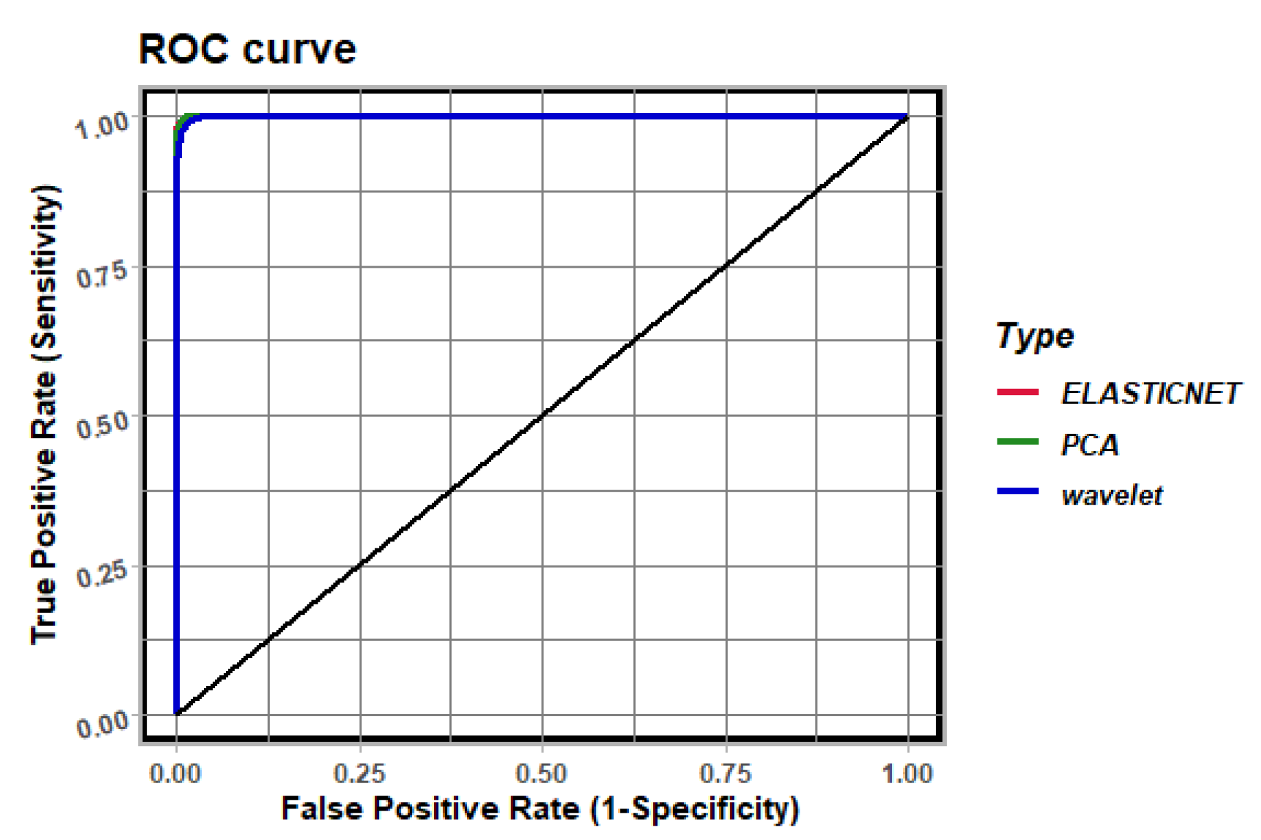
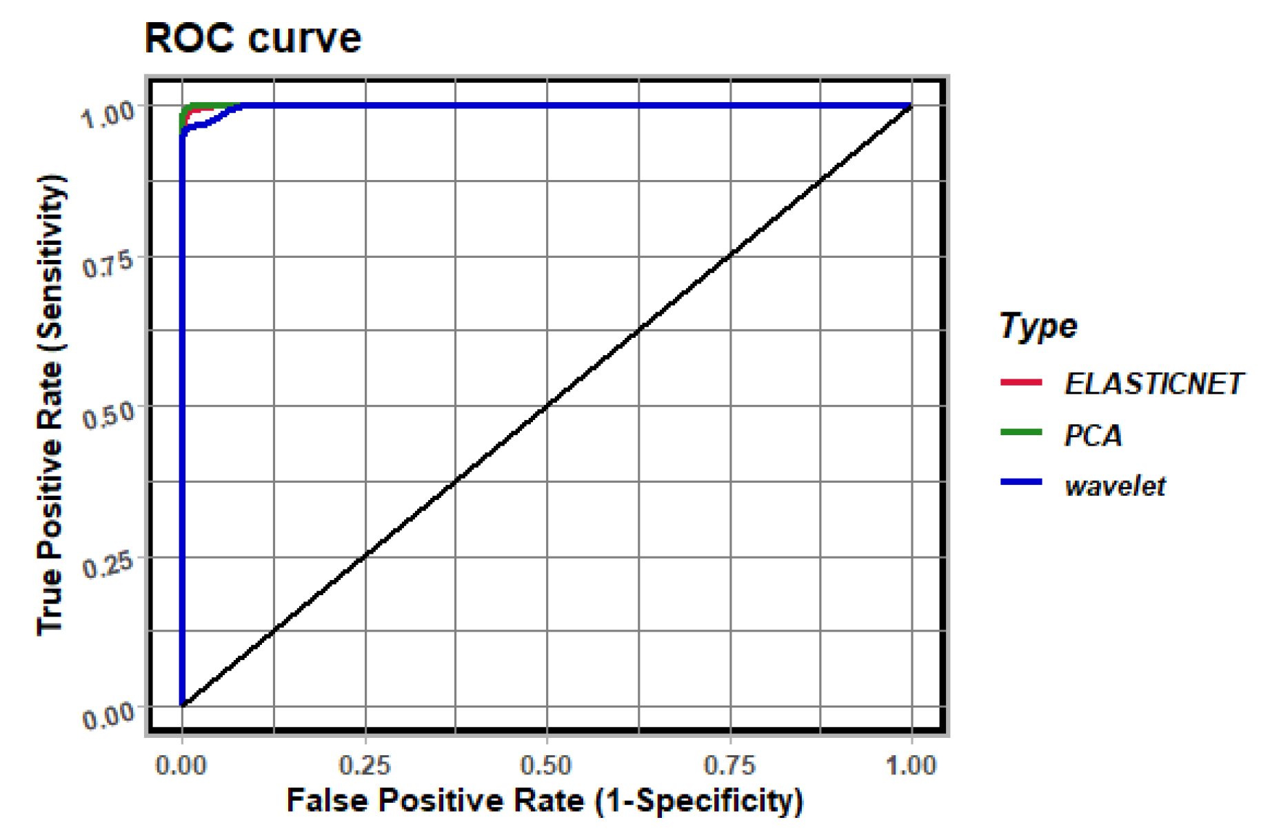
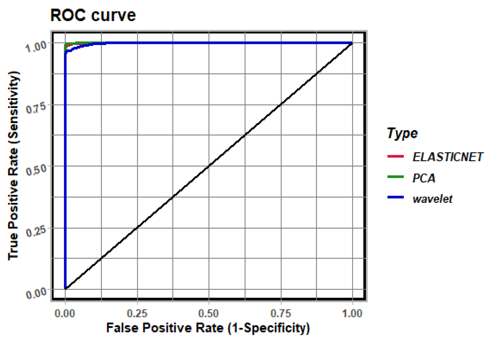
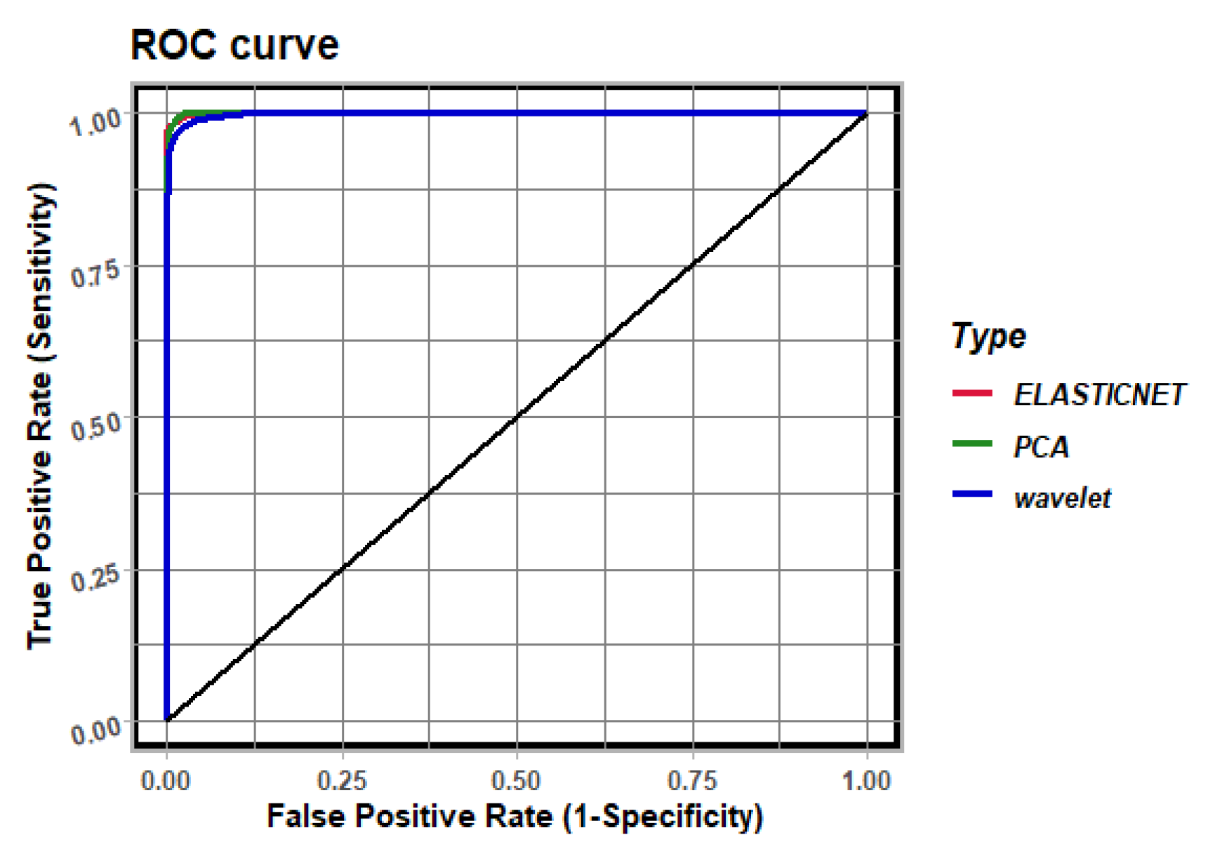
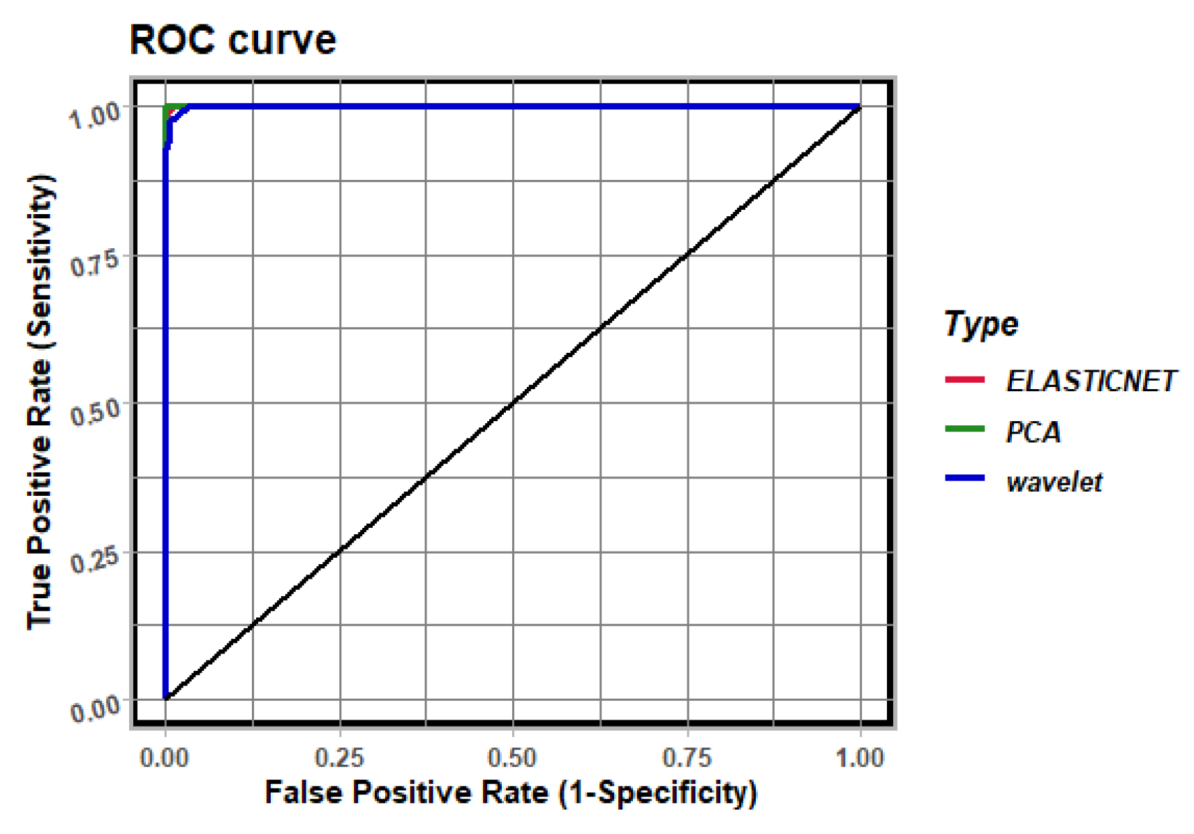
2.3.2. Receiver Operating Characteristic (ROC)

The viewing area consists of $k\in \mathbb{N}$ finite elements. A logistic regression model (3) is determined for each finite element. The obtained signal $X\in {ℝ}^m$ from the electrodes is used to estimate the probability of inclusion $P_j\left(Y=1|X\right)$ for j− finite element, 1 ≤ j ≤ k. The reconstruction of the viewing area is defined as a sequence ${\left\{{\widehat{z}}_j\right\}}_{1\le j\le k}$, where for cutting level $l\in \left(0, 1\right)$.

For the proper recognition of the visual area, coefficients describing the quality of the area recognition must be provided. For this purpose, it is assumed that a finite element that does not belong to the inclusions is described as a negative case (N); observing the problem at hand, this should be interpreted as a ground. On the other hand, if a finite element belongs to the inclusions and is in the inclusion area, this is taken as the positive case (P).

The confusion matrix is determined in the following way: TP (True Positive) denotes the finite elements that correctly belong to the inclusion area, TN (True Neg-ative) denotes the number of finite elements that are properly recognized as belonging to the background, FP (False Positive) denotes the number of finite elements belonging to the background that are recognized as having belonged to the inclusion area (false alarm), and FN (False Negative) denotes the number of finite elements belonging to the inclusion area but recognized as background (

Table 2. Positive and negative prediction.

	Positive	Negative
PositivePrediction	TP	FP
NegativePrediction	FN	TN

).

For each finite element, from the readings X, we determine the inclusion probability $P\left(Y=1|X\right)$ according to Equation (3) and assume for the level $l\in \left(0, 1\right)$.

The quality of image reconstruction (finding inclusions in the field of view) based on a classifier by logistic regression (3) is estimated by ratios [46,47]. The based ratios (coefficients) are determined as follows:

$$Accuracy=\frac{TP+TN}{TP+TN+FP+FN},$$

$$True Positive Rate=Sensivity=\frac{TP}{TP+FN},$$

$$Specificity=1-FalsePositiveRate=\frac{TN}{TN+FP},$$

$$PositivePredictiveValue=\frac{TP}{TP+FP},$$

$$NegativePredictiveValue=\frac{TN}{TN+FN},$$

$$DetectionRate=\frac{TP}{TP+TN+FP+FN},$$

The accuracy represents the part of the visual area that the model correctly recognises. Note that this is only one possible measure that represents the correctness of the recognition.

2.3.3. Elastic Net

Signals derived from EIT tomography electrodes can be collinear signals. Because such collinear variables may appear, the Elasticnet method for logistic regression was applied [26]. A possible regularisation method is an elastic net, defined as a linear mixture of a Selection Operator (LASSO), Least Absolute Shrinkage and ridge regression, which is called Tikhonov regularisation [52,53]. Instead of the solution of classical task (5), which is connected with an estimation of unknown parameters in the logistic regression model, we optimise the objective function (6) whilst taking the penalty into account. In order to do this, we need to solve the following equation:

$$\underset{\beta }{\max }\left\{{\displaystyle \sum }_{i=1}^N\left(y_i{x}_{\left(i\right)}\beta -\ln \left(1+e^{x_{\left(i\right)}\beta }\right)\right)-\lambda P_{\alpha }\left(\beta \right)\right\}$$

(9)

where λ > 0 denotes the regularisation ratio, and $0\le \alpha \le 1$, and $P_{\alpha }$ denotes the penalty, as follows:

$$P_{\alpha }\left(\beta \right)=\alpha {\left|\right|\beta \left|\right|}_{L_1}+\frac{1-\alpha }{2}{\left|\right|\beta \left|\right|}_{L_2}={\displaystyle \sum }_{j=1}^p\left(\alpha \left|{\beta }_j\right|+\frac{1-\alpha }{2}{\beta }_j^2\right)$$

(10)

The penalty $P_{\alpha }\left(\beta \right)$ is the combination of the linear norm of the parameter $\beta$ in $L_1$ and $L_2$ spaces. For $\alpha =0$ we have ridge regression, whereas for $\alpha =1$ we have LASSO regularisation.

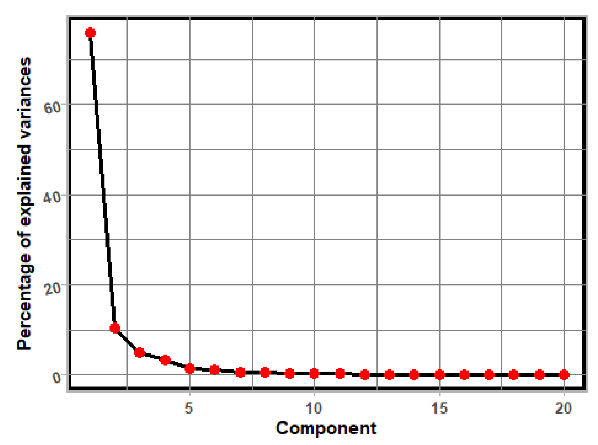
2.3.4. Principal Components Analysis

Principal Component Analysis involves identifying factors (components) present in a dataset X, [49,54]. This contains n observations for m variables. The aim of PCA is to rotate a coordinate solution in such a way as to maximise the variability of the first coordinate, followed by the variability of the next coordinate, and so on. The coordinates of the new system are called the charges of the generated principal components. In the new space, most of the variability is explained by the initial factors. PCA is frequently applied to reduce size of a dataset of statistics by discarding recent factors [50].

The decomposition of an X matrix is by Singular Value Decomposition. Thus, any real matrix X may be represented as

$$X=UD{V}^T+{\epsilon }_X$$

(11)

where $U\in R^{n\times m}$ is the left orthogonal matrix of left singular vectors, $D\in R^{m\times m}$ is the diagonal matrix containing the singular values, and $V\in R^{m\times m}$ is the right orthogonal vector matrix (matrix of right singular vectors). The orthogonal matrix V satisfies the property V^T = V⁻¹. The decomposition of a given matrix X may be shown as

$$X=T{P}^T+{\epsilon }_X$$

(12)

where T = UD denotes coordinates, and V = P denotes charges. A coordinate matrix T is determined by the multiplication of both sides (in a new space) of the equation $X=T{P}^T$ by P, obtaining

$$XP=T{P}^{T}P=T$$

(13)

According to the expansion (13), we find the weights that are used in the linear combination in the column V of the matrix to form the new dimensions. This formula expresses the variance of the coordinates in the new space:

$${\lambda }_i=\frac{d_i^2}{n-1}$$

(14)

where $d_i$ and $0\le i\le k$ are the singular values from the diagonal of matrix D. The part of the variance explained by the i-th principal component is $\frac{{\lambda }_i}{{{\displaystyle \sum }}_{j=1}^m{\lambda }_j}$, while the amount of variance that is explained by k principal components is $\frac{{{\displaystyle \sum }}_{j=1}^k{\lambda }_i}{{{\displaystyle \sum }}_{j=1}^m{\lambda }_j}$ for 1 ≤ k ≤ m.

Note that in EIT, for each case, the electrode readout including polarisation and projection angles $x_{\left(j\right)}\in R^m$ (according to (13)) corresponds to the value of $x_{\left(j\right)}P$ in the new space. The logistic regression of the form (2) is determined for individual finite elements, except that we analyse the linear dependence of the chance logarithm on a value in the new coordinates $\ln \theta \left(S\right)=T\beta +\epsilon$.

2.3.5. Discrete Wavelet Transformation (DWT)

Another method to reduce the amount of data that is redundant is to determine the projection of the signal ${\left\{x_t\right\}}_{1\le tleqm}$ obtained from the electrodes to an orthogonal basis named as the mother wavelet. By definition, $\Psi \left(t\right)$ will be an orthogonal wavelet basis. For $j\in \mathbb{Z}$, the sequence is defined as

$${\Psi }_{jk}\left(t\right)=\frac{1}{2^{j-1}}\Psi \left(\frac{t}{2^j}-k\right)$$

(15)

and ${\left\{{\varphi }_{jk}\right\}}_{k\in \mathbb{Z}}$

$${\varphi }_{jk}\left(t\right)=\frac{1}{2^{j-1}}\varphi \left(\frac{t}{2^j}-k\right)$$

(16)

where $\varphi \left(t\right)$ denotes the scaling function which corresponds to the parent wavelet $\Psi$. In this case, the time series ${\left\{x_t\right\}}_{1\le tleqm}$ can be represented as

$$x_t={\displaystyle \sum }_{k=-\infty }^{\infty }{c}_{jk}{\varphi }_{jk}\left(t\right)+{\displaystyle \sum }_{i=-\infty }^j{\displaystyle \sum }_{k=-\infty }^{\infty }{d}_{ik}{\Psi }_{ik}\left(t\right)$$

(17)

where the value $c_{jk}$ is the scaling factor, but d_ik is the specific coefficient. Sequence ${\left\{x_t\right\}}_{1\le tleqm}$ can be expressed in a different form from the level of decomposition $j\in \mathbb{Z}$ based on Equation (17).

The functions ${\Psi }_{jk}\left(t\right)$ and ${\varphi }_{jk}\left(t\right)$ take values which are different from zero on a bounded interval. It follows that the sequence ${\left\{x_t\right\}}_{1\le t\le m}$ can be presented as follows:

$$x_t={\displaystyle \sum }_{k=0}^s{c}_{jk}{\varphi }_{jk}\left(t\right)+{\displaystyle \sum }_{i=0}^j{\displaystyle \sum }_{k=0}^s{d}_{ik}{\Psi }_{ik}\left(t\right)$$

(18)

where $s<<m$. According to [28], a projection operator for a time series is defined as ${\left\{x_t\right\}}_{1\le t\le m}$ at level $j$ on an orthogonal basis ${\left\{{\varphi }_{jk}\left(t\right)\right\}}_{0\le k\le s}$, as follows:

$$P^j{x}_t={\displaystyle \sum }_{k=0}^{\frac{n}{2^j}-1}{c}_{jk}{\varphi }_{jk}\left(t\right)$$

(19)

Much information on DWT can be read in [28,55,56]. The EIT for the sequence of scaling factors from the projection (26) was used as the input variables for the logistic regression. There are different types of wavelet, e.g., Daubechies (‘db1’–‘db18’), Coiflets (‘coif1’–‘coif5’), Symlets (‘sym1’–‘sym18’) and Biorthogonal (‘bior1.1’, ‘bior1.3’, ‘bior1.5’, ‘bior2.2’, ‘bior2.4’, ‘bior2.6’, ‘bior2.8’). Some results are presented in the next section.

To analyse this, we used Daubechies1 decomposition, which is also known as a Haar wavelet. The mother wavelet is defined as follows:

$$\Psi \left(t\right)=\{\begin{array}{ll}1,\hfill & t\in \left[0,\frac{1}{2}\right),\hfill \\ -1,\hfill & t\in \left[\frac{1}{2},1\right),\hfill \\ 0,\hfill & t\notin \left[0,1\right)\hfill \end{array}$$

(20)

but corresponding to her, the father wavelet is defined as follows:

$$\varphi \left(t\right)=\{\begin{array}{ll}1,\hfill & t\in \left[0,1\right),\hfill \\ 0,\hfill & t\notin \left[0,1\right).\hfill \end{array}$$

(21)

From (15) and (16), we see that the coefficients ${\Psi }_{jk}\left(t\right)$ and ${\varphi }_{jk}\left(t\right)$ have different-from-zero values at the interval $\left[2^{j}k,2^j\left(k+1\right)\right)$.

2.3.6. Algorithm Implementation

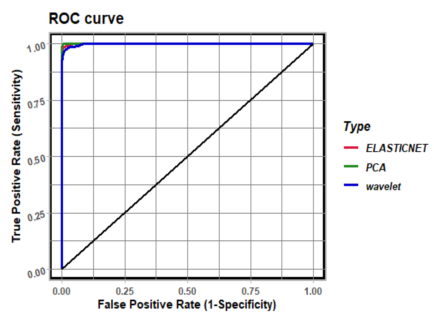
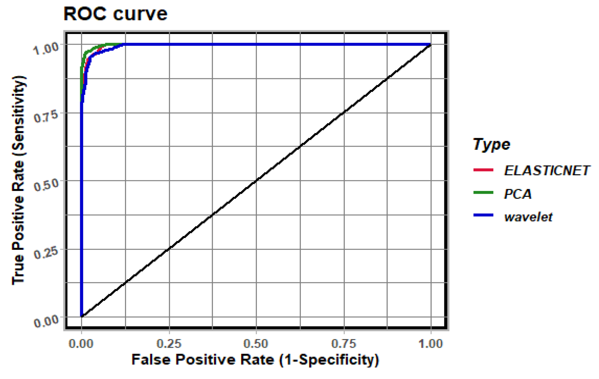
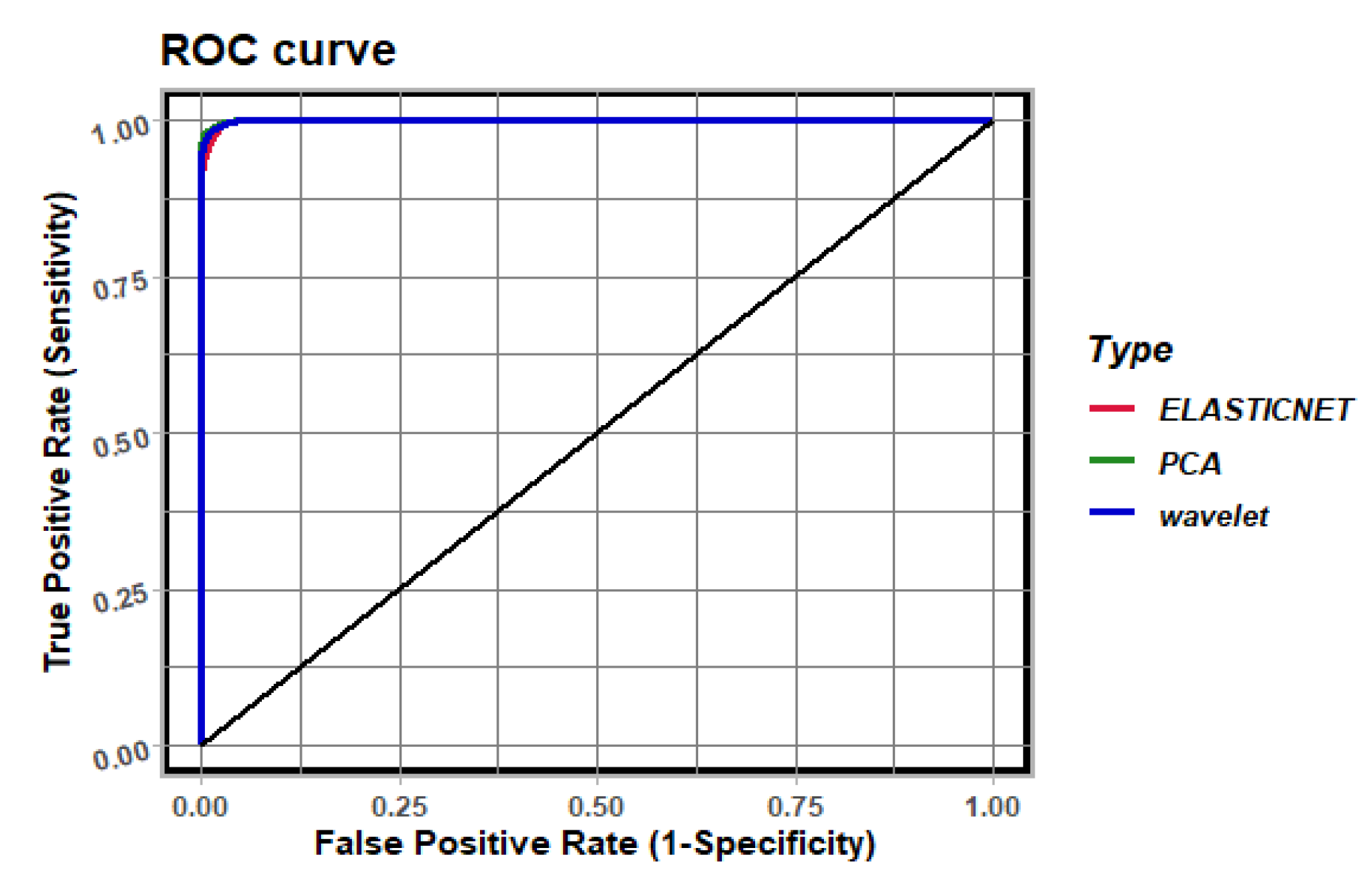
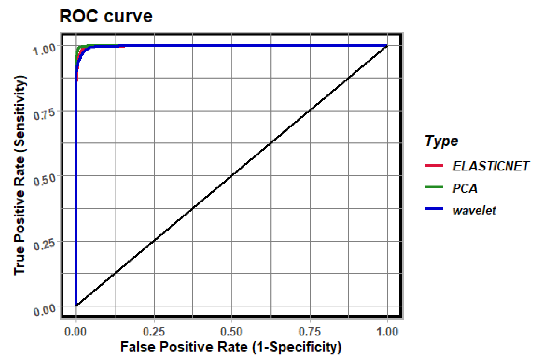
In the classical inverse problem in EIT, we determine the conductivity of each finite element located in the viewing area. Our approach was to determine the inclusions with high probability areas; logistic regression was used for this purpose. The main problem in EIT is the problem of the co-liveness of features (measurements from electrodes). It is impossible to extract a set of stochastically independent features. In order to improve the quality of the classifier, the following techniques were additionally applied: elastic net regularization, principal component analysis and wavelet preprocessing. In this paper, however, only one type of wavelet was used, analyzing the accuracy and AUC curves. This technique is more robust to perturbations of the measurements from the electrodes. Figure 6 shows the learning process of the algorithm, while Figure 7 shows the reconstruction process using machine learning methods.

3. Results

This chapter presents water leakage results from dikes based on the built numerical models and laboratory measurements. Three models of tomographic image reconstruction systems were developed. The results of the presented solutions are presented in this chapter. The inverse and ill-posed problems of electrical tomography are related to the insufficient number of function arguments (measurements/inputs) compared to the required number of outputs (image pixels).

The presented research aims to generate a spatial image of the moisture with a specific pixel resolution from the measurements. Single models are trained with all of the measurement values as the input and only a one-pixel value as the output in order to simplify the generation of multi-pixel images. Therefore, the algorithm must generate as many models as there are pixels in the image. When learning the predictive models, each model obtains different coefficients and hyperparameters that determine the ways in which the input values are transformed to the output.

In the models presented below for each finite element, we determined the model of logistic regression. The measurements obtained from the electrodes are collinear. Thus, the direct application of logistic regression implies that the absolute values of the structural parameters of regression are quite large, and the prediction is poor. Therefore, three approaches were applied to overcome the collinearity problem of the input variables: (1) elastic net regularisation, (2) the estimation of the principal component measurements (PCA application) as input variables in the regression model, (3) the projection of the measurements obtained from the electrodes based on wavelet decomposition at level $4$.

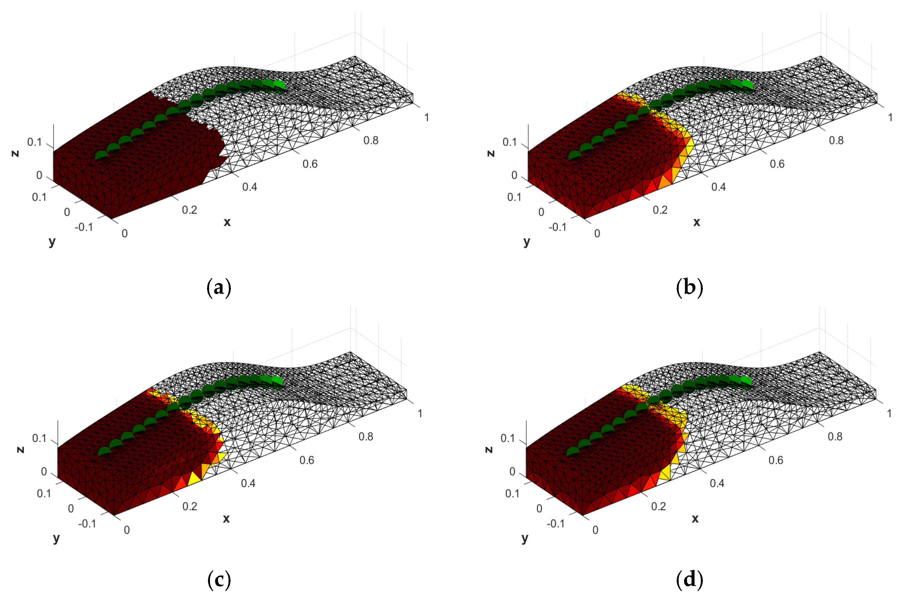
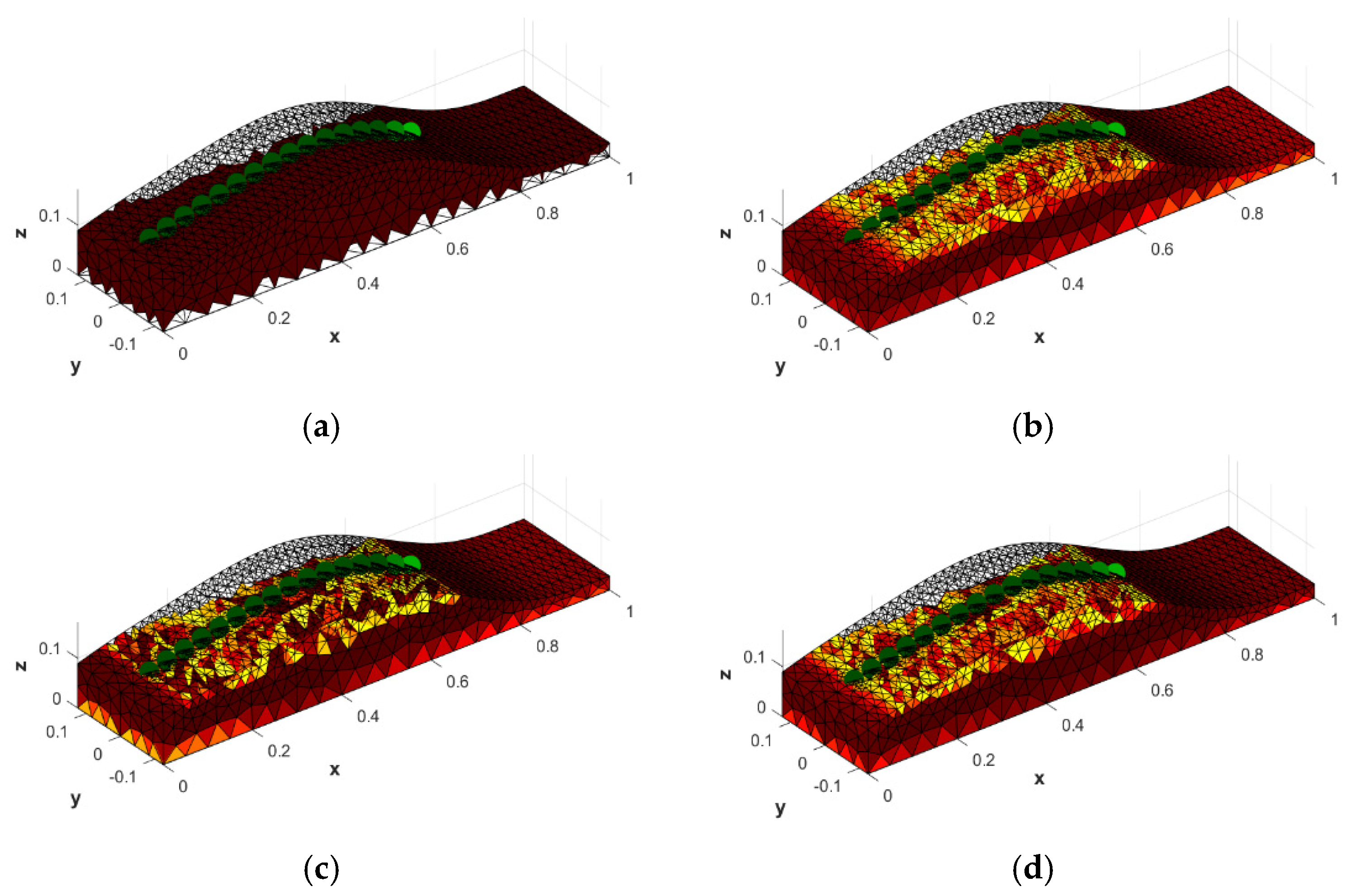
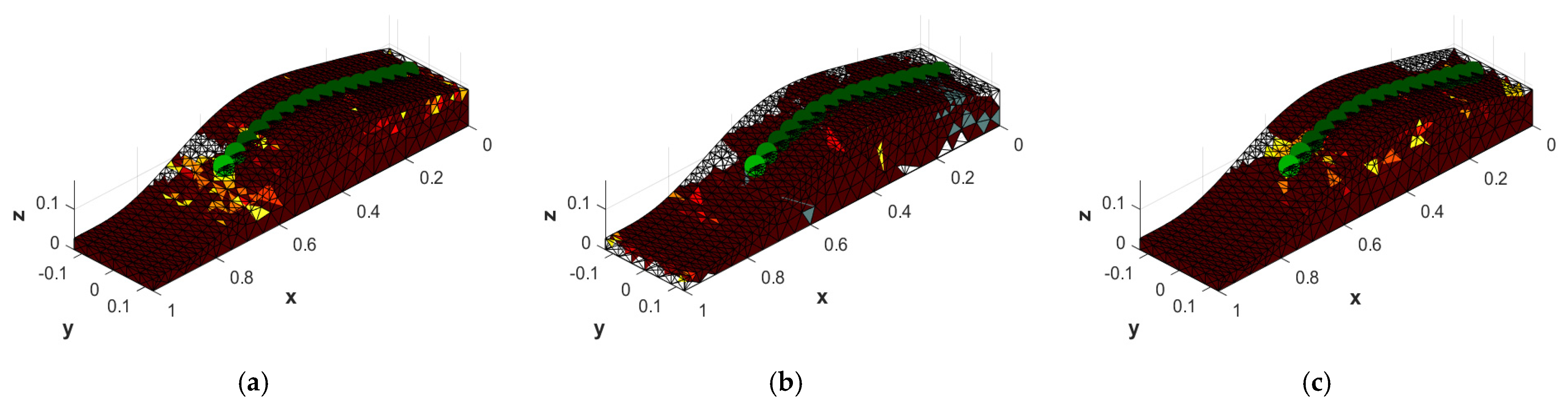
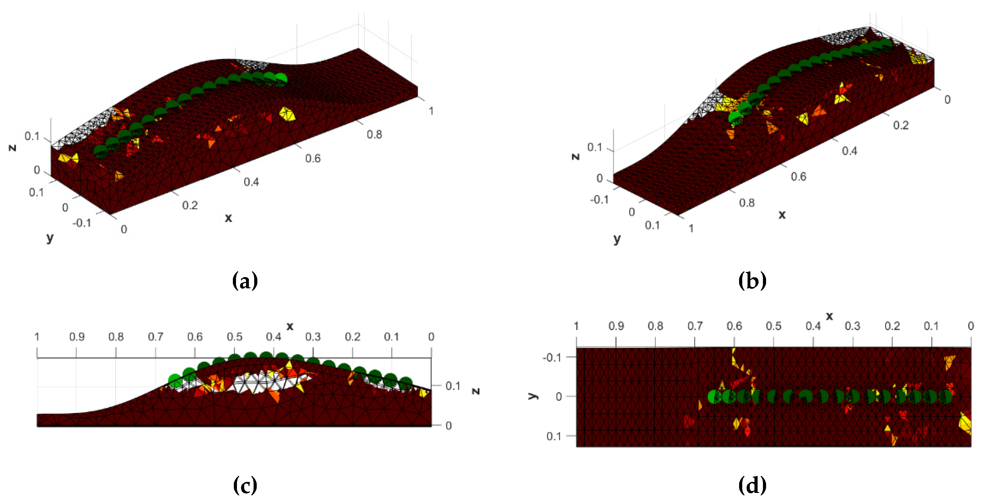
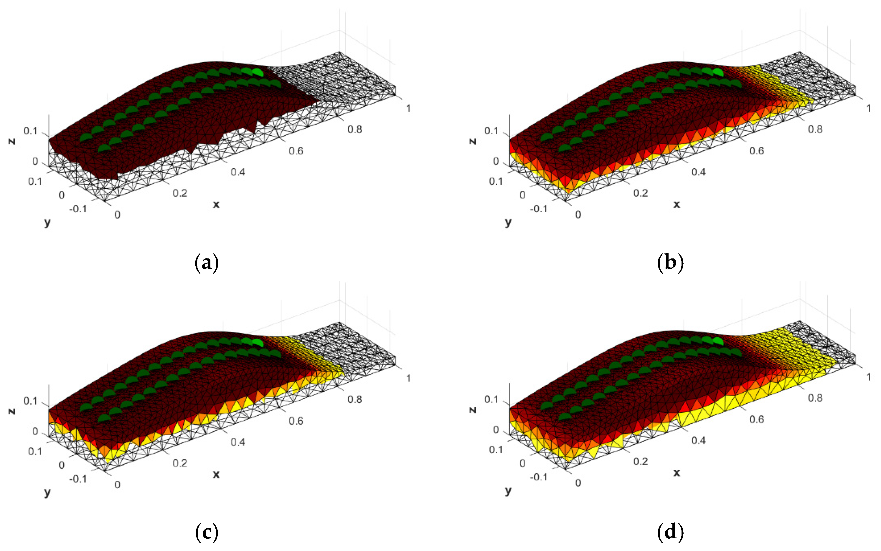
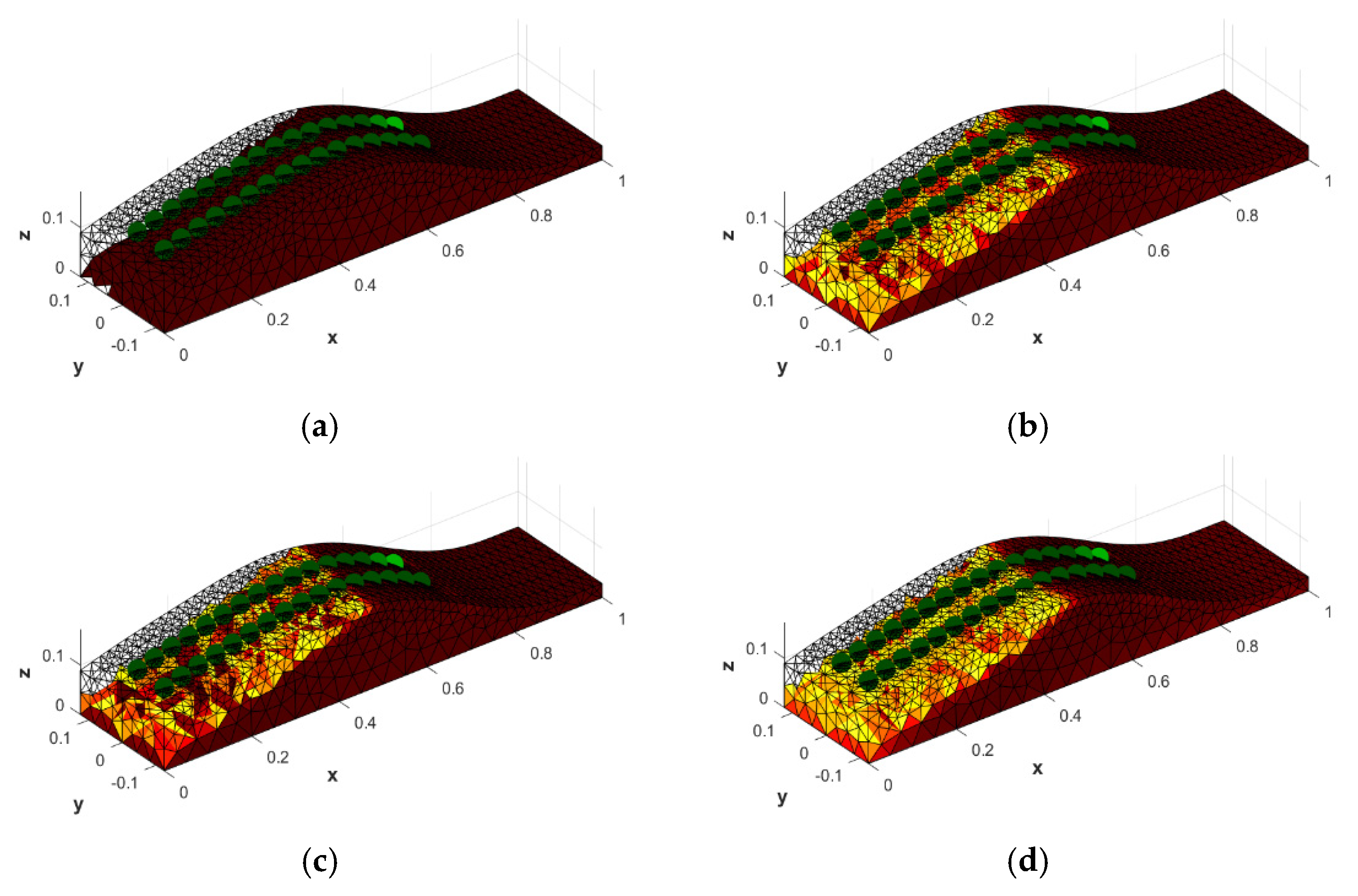
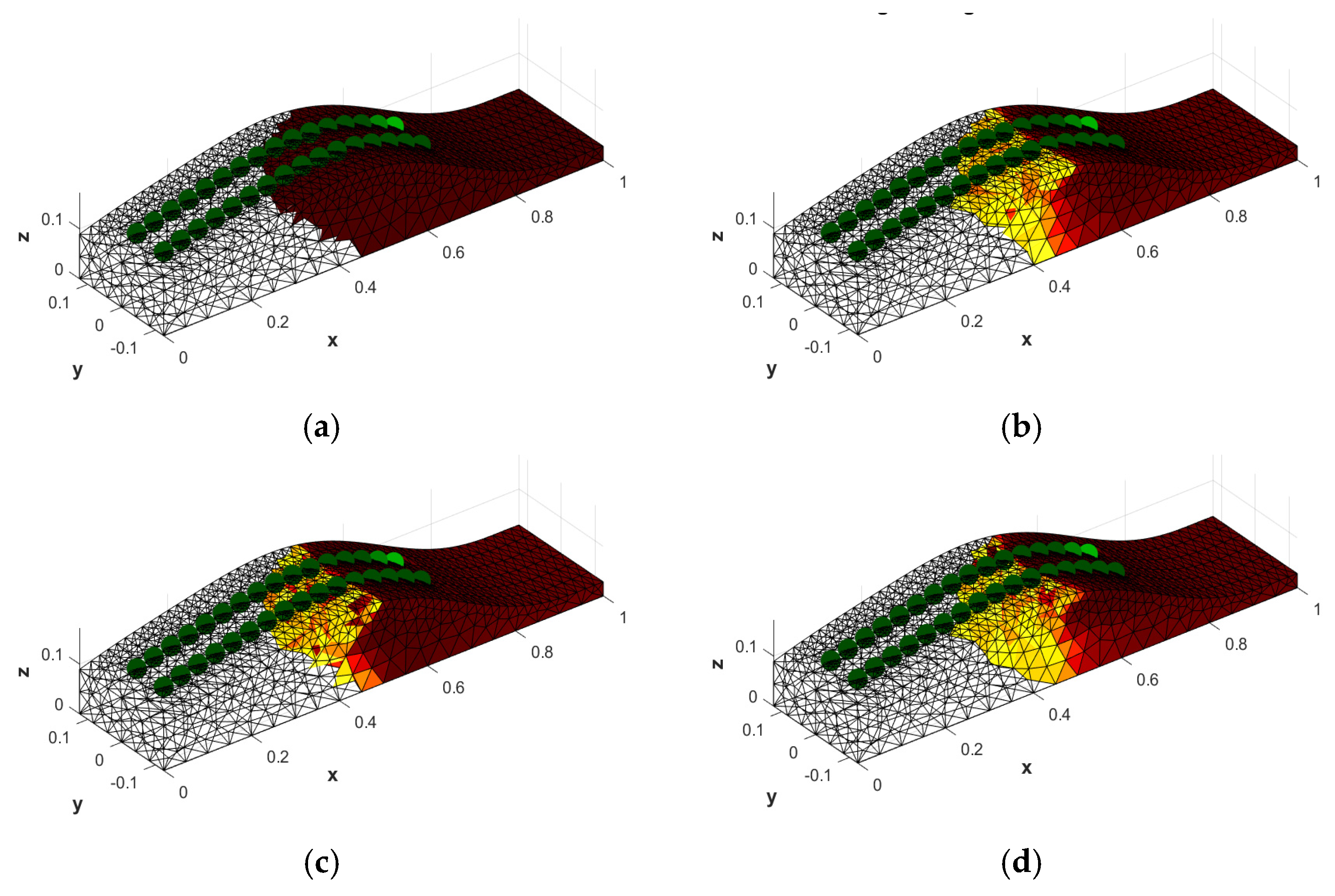
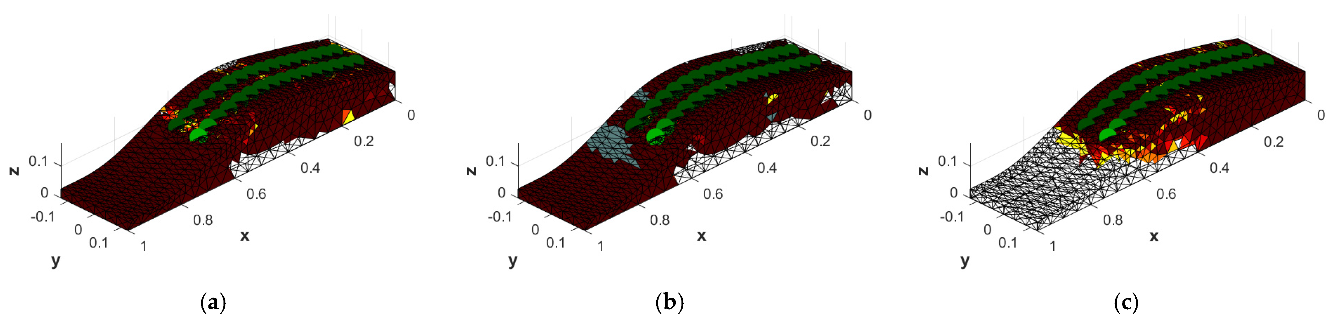
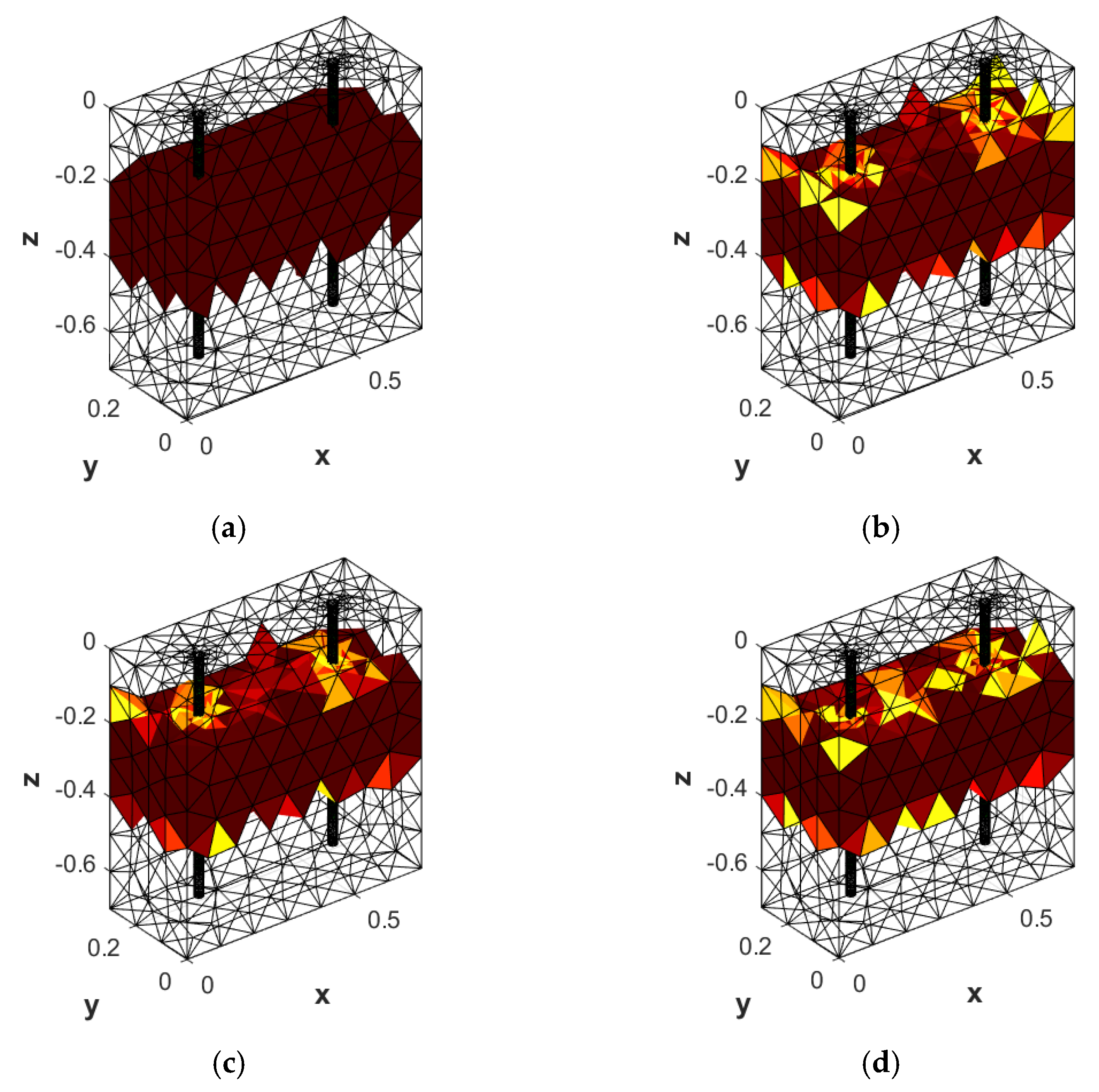
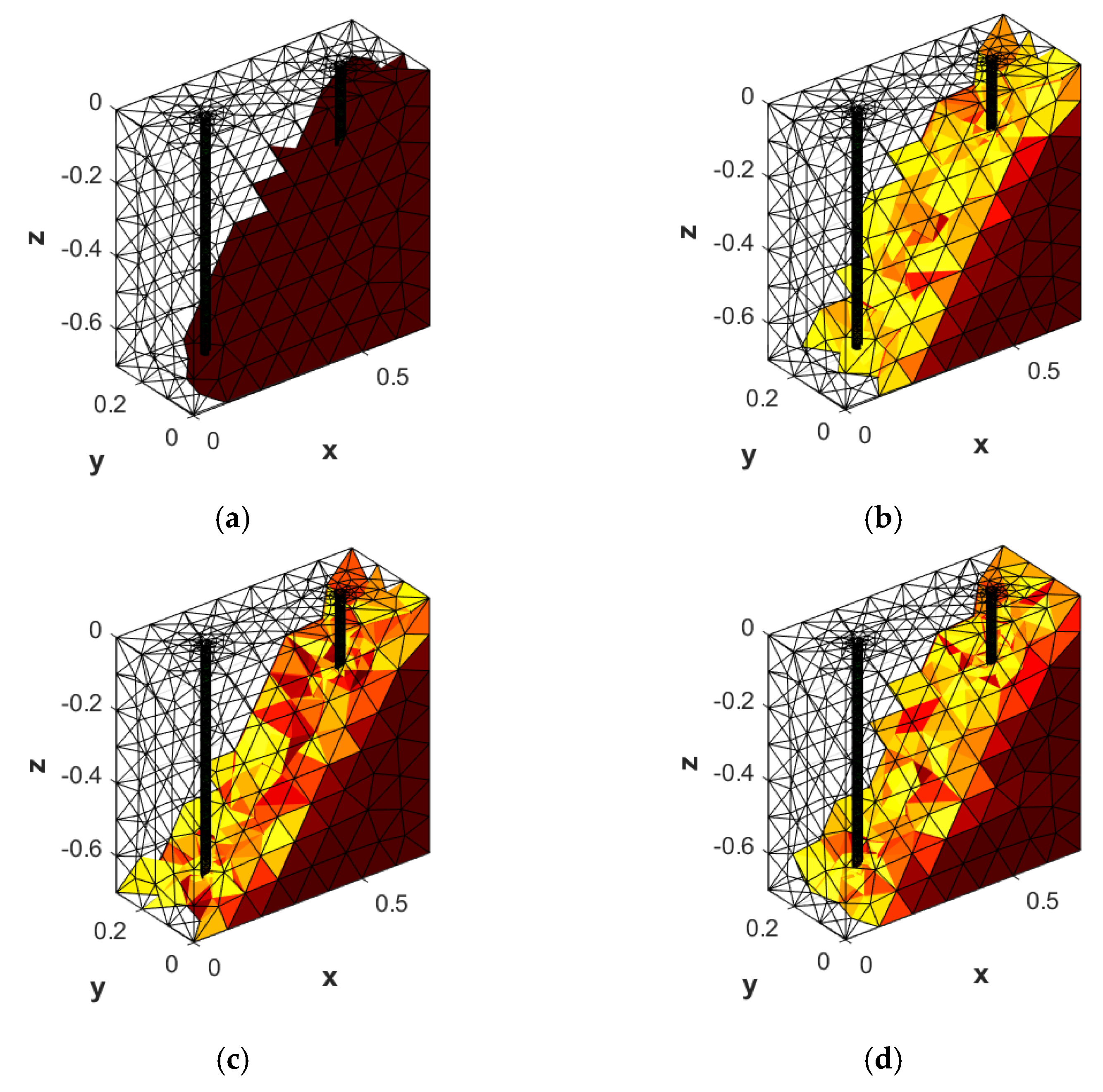
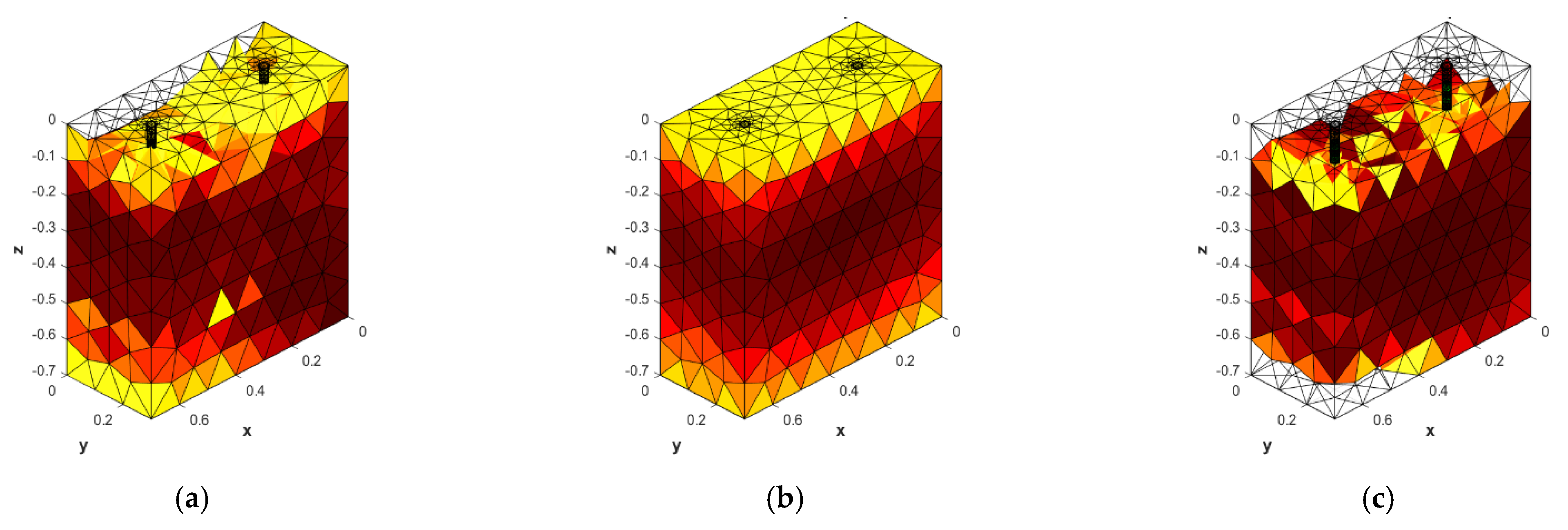
3.1. Image Reconstruction for Model I

Figure 8 shows a numerical model of a dike with electrodes placed on its surface in one row. Model I consists of 16 electrodes, 2159 nodes, 7657 finite elements and point electrodes. Figure 9, Figure 10, Figure 11, Figure 12, Figure 13 and Figure 14 summary the image reconstruction for Model I. Figure 9, Figure 11 and Figure 13 show 3 cases of the reconstruction of the flood embankment image for model I, with different variants of water infiltration, divided into the methods of logistic regression with an elastic net, logistic regression with PCA distribution, and regression logistic with wavelet distribution.

Table 3. The basic characteristic of reconstruction for model I—example 1.

	Elasticnet	PCA	Wave
Sensitivity	0.9697954	0.9808379	0.9632998
Specificity	0.9984709	0.9997816	0.9912626
Pos Pred Value	0.9976612	0.9996690	0.9866933
Neg Pred Value	0.9800600	0.9872735	0.9757041
Precision	0.9976612	0.9996690	0.9866933
Recall	0.9697954	0.9808379	0.9632998
F1	0.9835310	0.9901639	0.9748562
Prevalence	0.4021157	0.4021157	0.4021157
Detection Rate	0.3899700	0.3944103	0.3873580
Detection Prevalence	0.3908842	0.3945409	0.3925820
Balanced Accuracy	0.9841332	0.9903097	0.9772812
AUC	0.9995741	0.9998988	0.9980552

,

Table 4. The basic characteristic of the reconstruction for model I—example 2.

	Elasticnet	PCA	Wave
Sensitivity	0.9746222	0.9923011	0.9751925
Specificity	0.9966265	0.9975904	0.9795181
Pos Pred Value	0.9959207	0.9971347	0.9757489
Neg Pred Value	0.9789349	0.9935205	0.9790462
Precision	0.9959207	0.9971347	0.9757489
Recall	0.9746222	0.9923011	0.9751925
F1	0.9851564	0.9947120	0.9754706
Prevalence	0.4580123	0.4580123	0.4580123
Detection Rate	0.4463889	0.4544861	0.4466501
Detection Prevalence	0.4482173	0.4557921	0.4577511
Balanced Accuracy	0.9856243	0.9949457	0.9773553
AUC	0.9994711	0.9999436	0.9983900

and

Table 5. The basic characteristic of the reconstruction for model I—example 3.

	Elasticnet	PCA	Wave
Sensitivity	1.0000000	0.9989063	0.9963544
Specificity	0.8658934	0.9277574	0.8858364
Pos Pred Value	0.8062904	0.8852989	0.8296903
Neg Pred Value	1.0000000	0.9993424	0.9977080
Precision	0.8062904	0.8852989	0.8296903
Recall	1.0000000	0.9989063	0.9963544
F1	0.8927583	0.9386776	0.9054166
Prevalence	0.3582343	0.3582343	0.3582343
Detection Rate	0.3582343	0.3578425	0.3569283
Detection Prevalence	0.4442993	0.4042053	0.4301946
Balanced Accuracy	0.9329467	0.9633319	0.9410954
AUC	0.9965007	0.9984147	0.9947318

show the results of the exact reconstructions shown in Figure 9, Figure 11 and Figure 13. The accuracy of the statistical ROC model for model I is evaluated in Figure 10, Figure 12 and Figure 14.

The analysis of the reconstruction’s accuracy to the disturbances arising in the measurement obtained from the electrodes signals using the method mentioned above will be presented in Figure 15. For this purpose, instead, for a reconstruction based on signal $x\in {ℝ}^m$ we analysed the reconstruction based on a disturbed signal $x+\sigma \epsilon$, where $\sigma \ge 0$ and $\epsilon :\Omega \to {ℝ}^m$ is a sequence of independent identically distributed random variables with normal distribution $N\left(0,1\right)$. The figure below shows the relationship between the accuracy and AUC (area under the curve) depending on the value $\sigma$ (standard deviation of disturbances).

In order to verify the performed numerical tests, a laboratory model of the flood embankment was prepared (shown in Figure 16), which was flooded with water. The image reconstruction results for the machine learning methods are shown in Figure 17, Figure 18, Figure 19 and Figure 20.

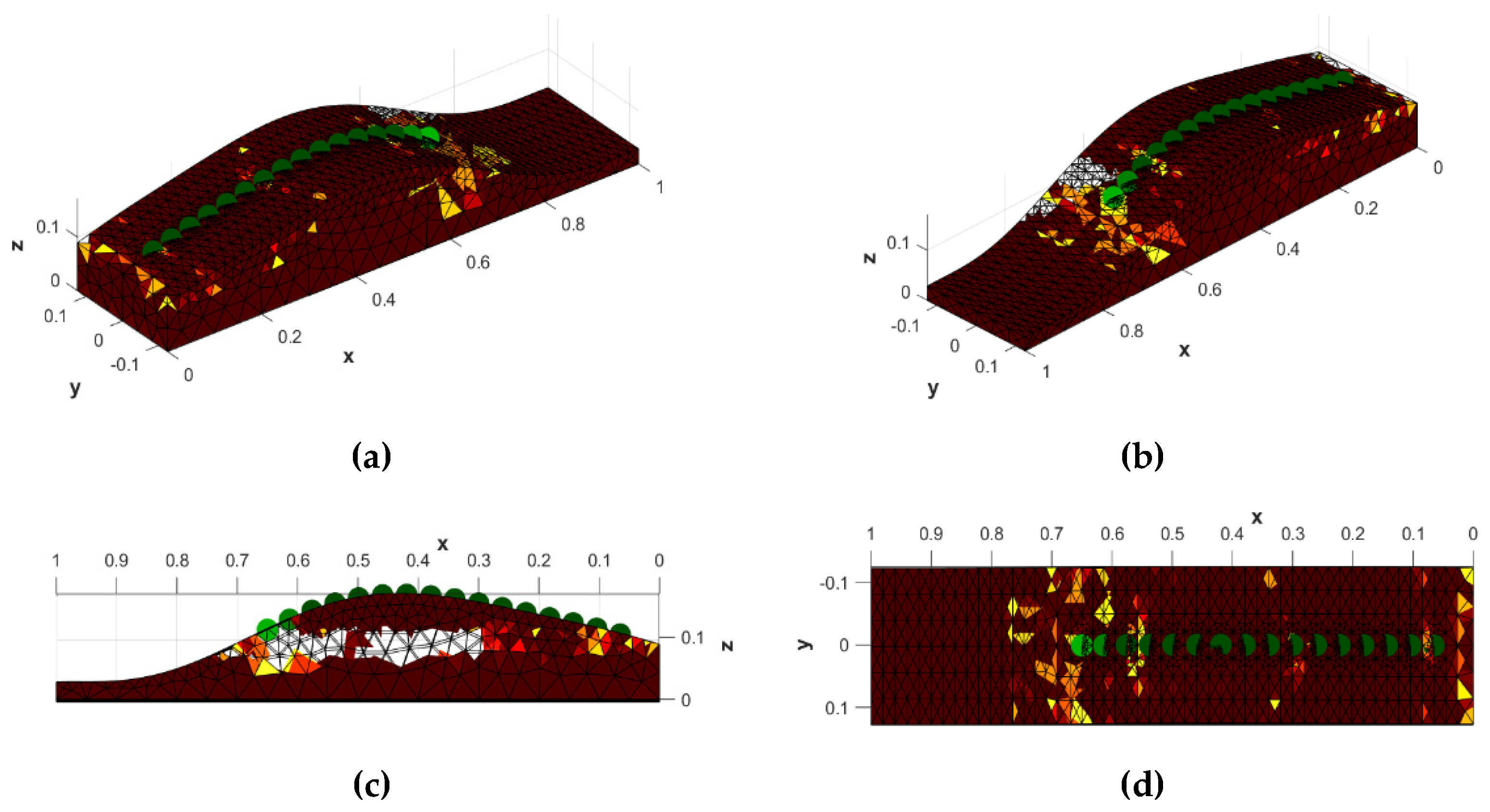
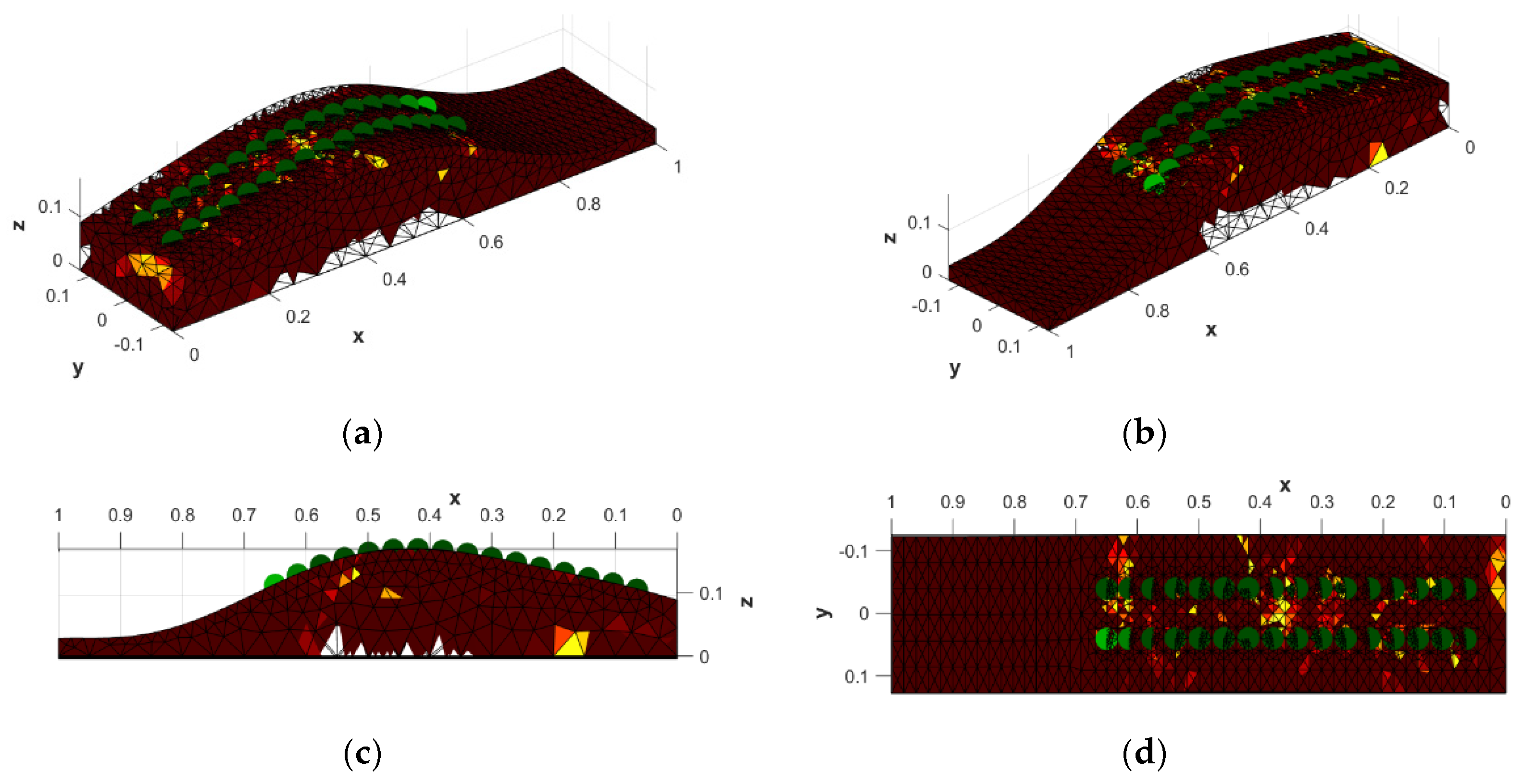
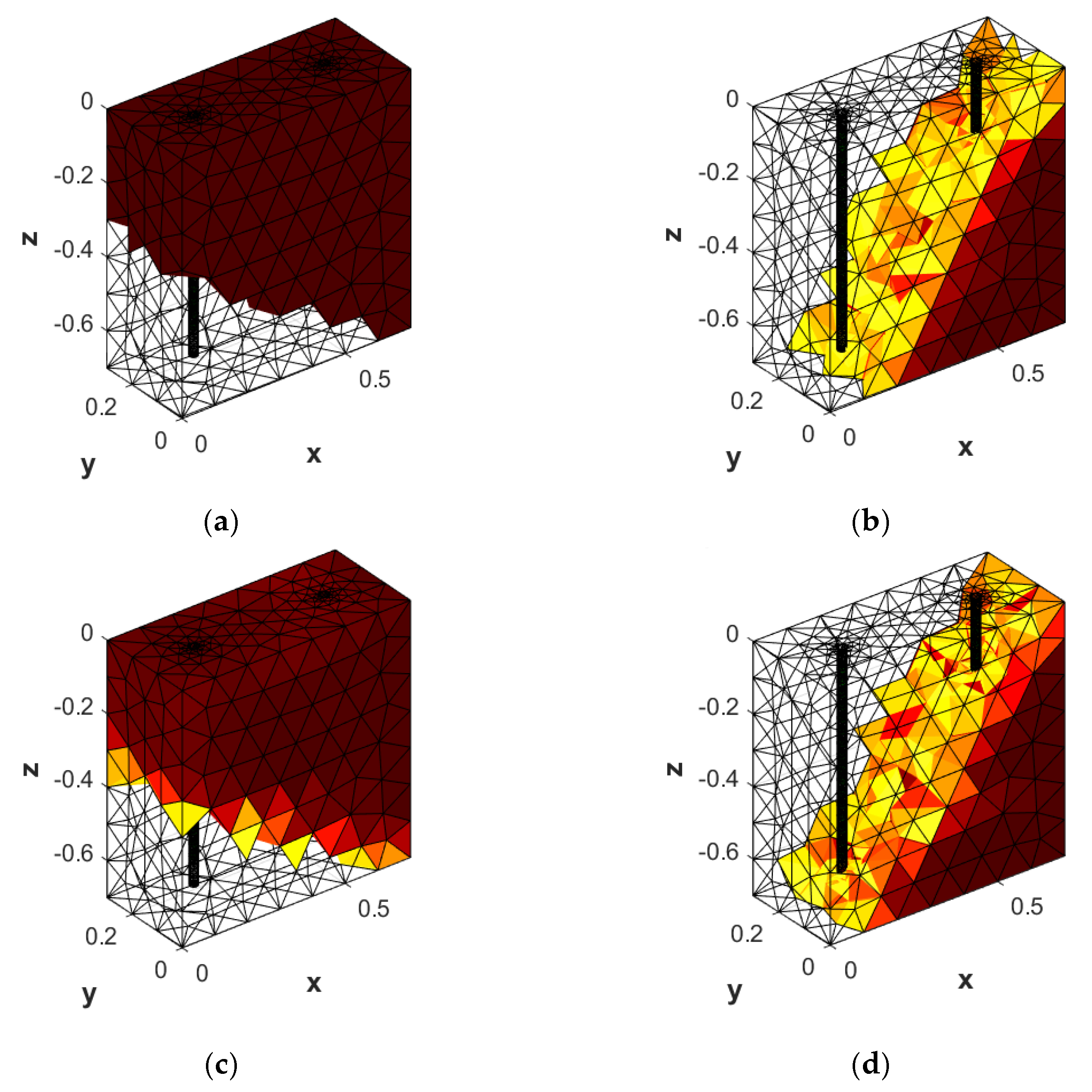
3.2. Image Reconstruction for Model II

Figure 21 shows a numerical model of a dike with electrodes placed on its surface in one row. Model I consists of 32 electrodes, 2818 nodes, 9805 finite elements and point electrodes. Figure 22, Figure 23, Figure 24, Figure 25, Figure 26 and Figure 27 summary the image reconstruction for Model II. Figure 22, Figure 24 and Figure 26 show three cases of image reconstruction for flood embankments of image reconstruction cases. The examples from model II have different variants of water infiltration divided into logistic regression methods with an elastic net, logistic regression with PCA distribution, and logistic regression with wavelet distribution.

Table 6. The basic characteristics of the reconstruction for model II—example 4.

	Elasticnet	PCA	Wave
Sensitivity	1.0000000	1.0000000	1.0000000
Specificity	0.7619853	0.9125776	0.7507050
Pos Pred Value	0.9500828	0.9810675	0.9478405
Neg Pred Value	1.0000000	1.0000000	1.0000000
Precision	0.9500828	0.9810675	0.9478405
Recall	1.0000000	1.0000000	1.0000000
F1	0.9744025	0.9904433	0.9732219
Prevalence	0.8191739	0.8191739	0.8191739
Detection Rate	0.8191739	0.8191739	0.8191739
Detection Prevalence	0.8622132	0.8349822	0.8642529
Balanced Accuracy	0.8809927	0.9562888	0.8753525
AUC	0.9995332	0.9998610	0.9978940

,

Table 7. The basic characteristics of the reconstruction for model II—example 5.

	Elasticnet	PCA	Wave
Sensitivity	0.9912896	0.9893775	0.9923518
Specificity	0.9784229	0.9856807	0.9354649
Pos Pred Value	0.9769682	0.9845666	0.9342000
Neg Pred Value	0.9918473	0.9901478	0.9925078
Precision	0.9769682	0.9845666	0.9342000
Recall	0.9912896	0.9893775	0.9923518
F1	0.9840768	0.9869662	0.9623983
Prevalence	0.4800612	0.4800612	0.4800612
Detection Rate	0.4758797	0.4749618	0.4763896
Detection Prevalence	0.4870984	0.4824069	0.5099439
Balanced Accuracy	0.9848562	0.9875291	0.9639084
AUC	0.9994805	0.9994952	0.9978997

and

Table 8. The basic characteristics of the reconstruction for model II—example 6.

	Elasticnet	PCA	Wave
Sensitivity	0.9705573	0.9826498	0.9613565
Specificity	1.0000000	0.9973338	0.9951675
Pos Pred Value	1.0000000	0.9957379	0.9921324
Neg Pred Value	0.9816784	0.9890927	0.9759765
Precision	1.0000000	0.9957379	0.9921324
Recall	0.9705573	0.9826498	0.9613565
F1	0.9850587	0.9891506	0.9765020
Prevalence	0.3879653	0.3879653	0.3879653
Detection Rate	0.3765426	0.3812341	0.3729730
Detection Prevalence	0.3765426	0.3828659	0.3759306
Balanced Accuracy	0.9852787	0.9899918	0.9782620
AUC	0.9998313	0.9998497	0.9993635

show the results of the exact reconstructions, as shown in Figure 22, Figure 24 and Figure 26. The accuracy of the ROC statistical model for Model II is evaluated in Figure 23, Figure 25 and Figure 27.

Figure 28 shows an analysis of the reconstruction accuracy of the perturbations arising in the measurements obtained from the electrode signals. The image reconstruction results for the machine learning methods are shown in Figure 29, Figure 30, Figure 31 and Figure 32.

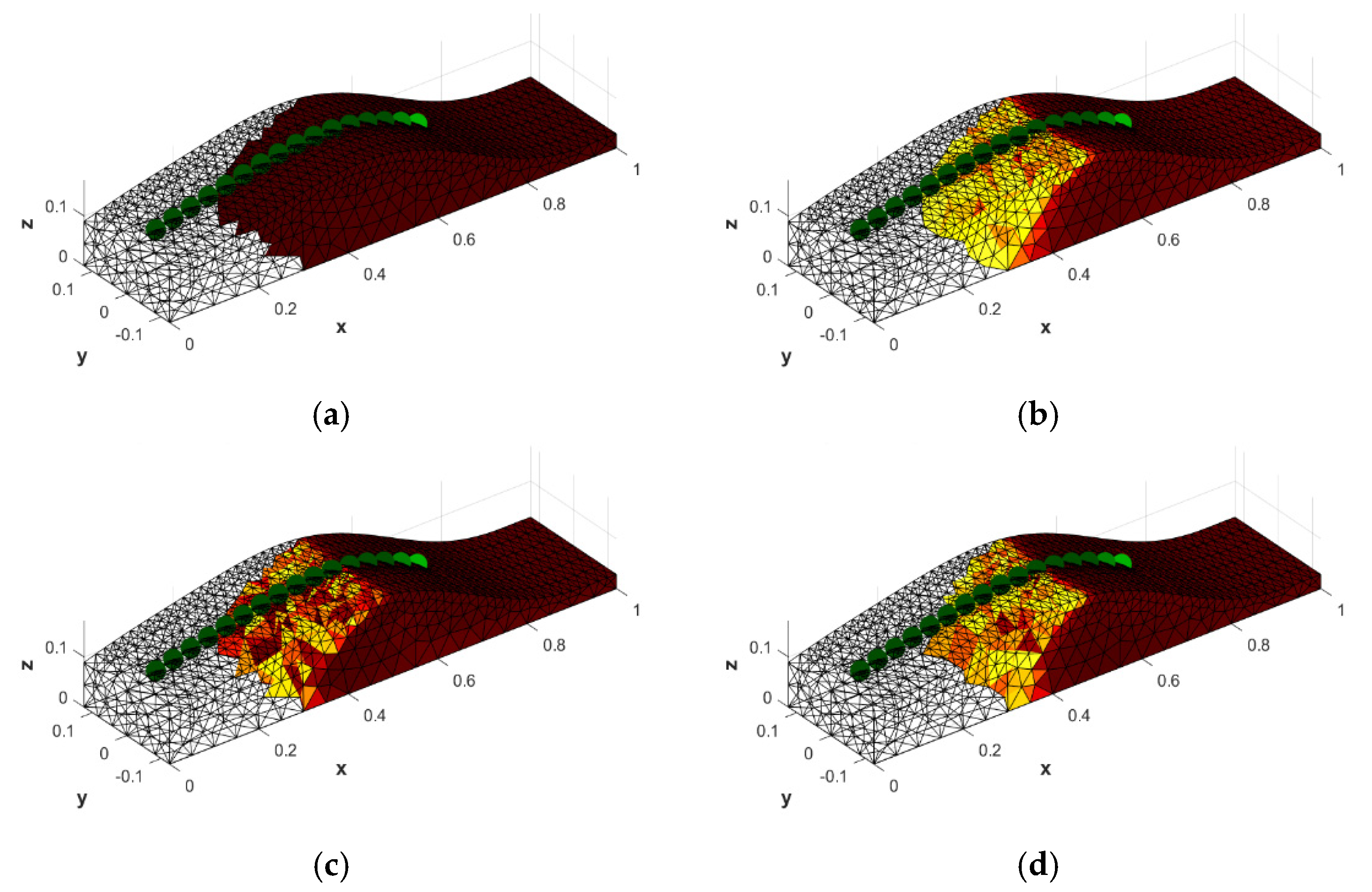
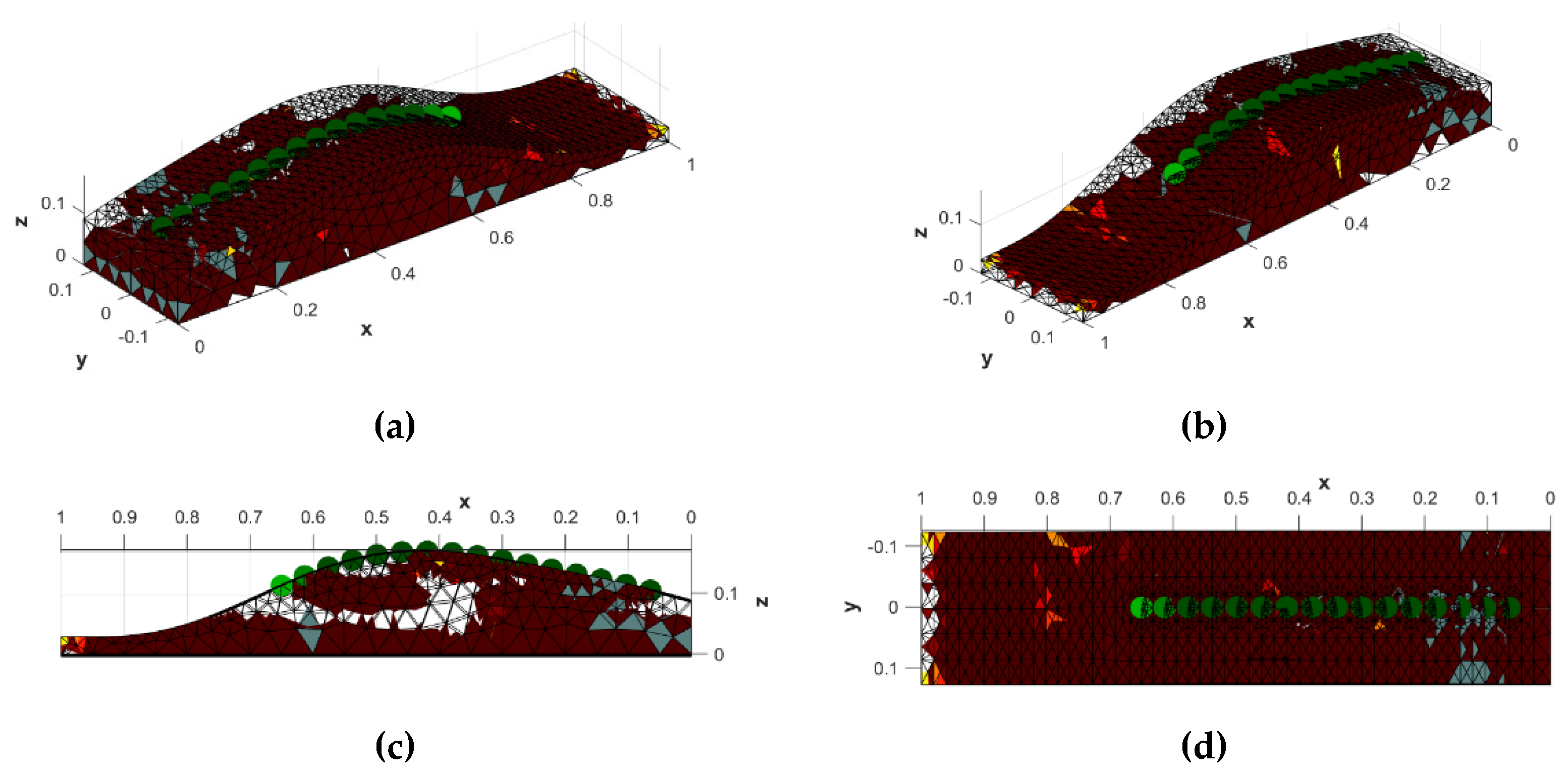
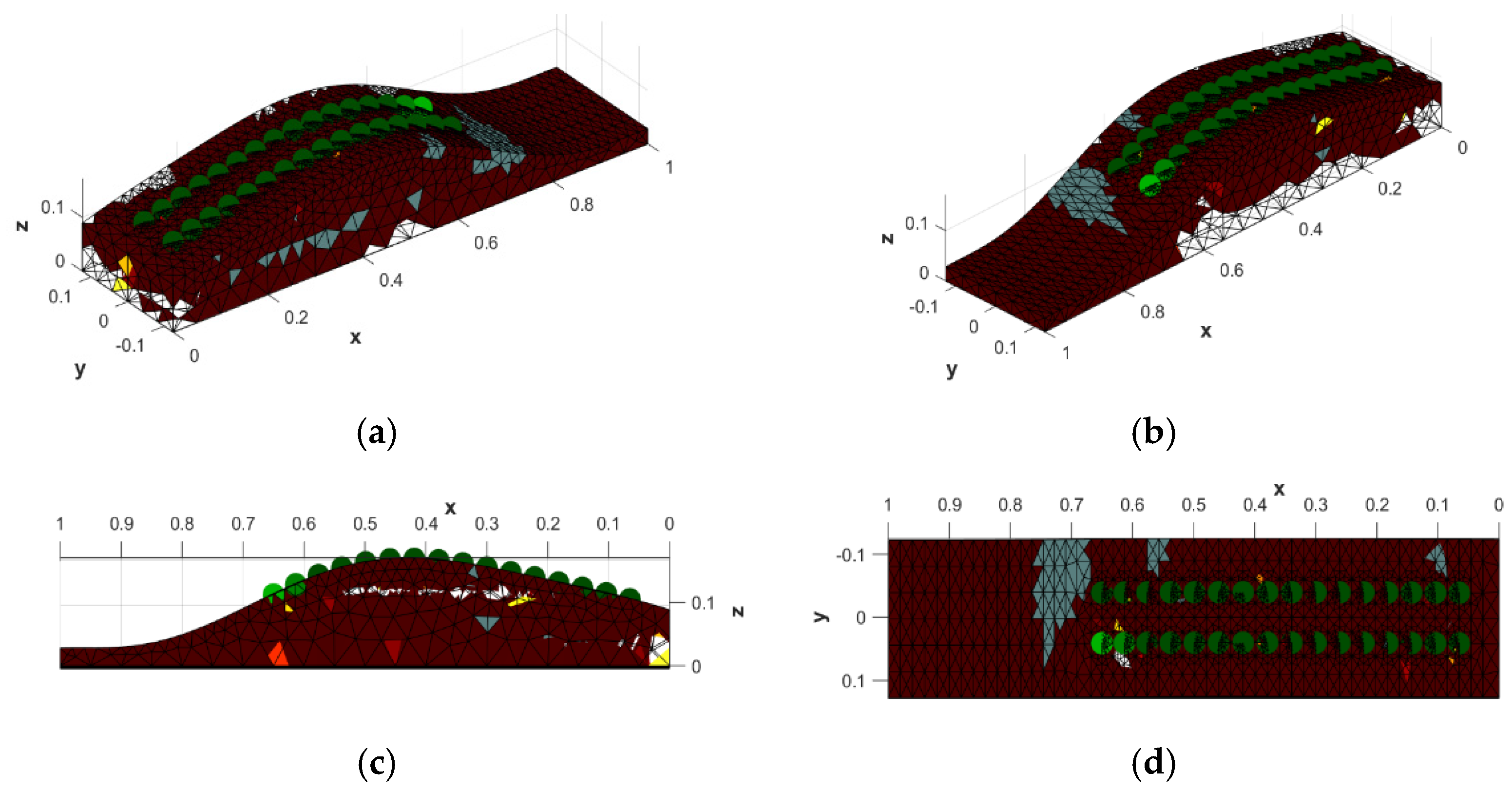
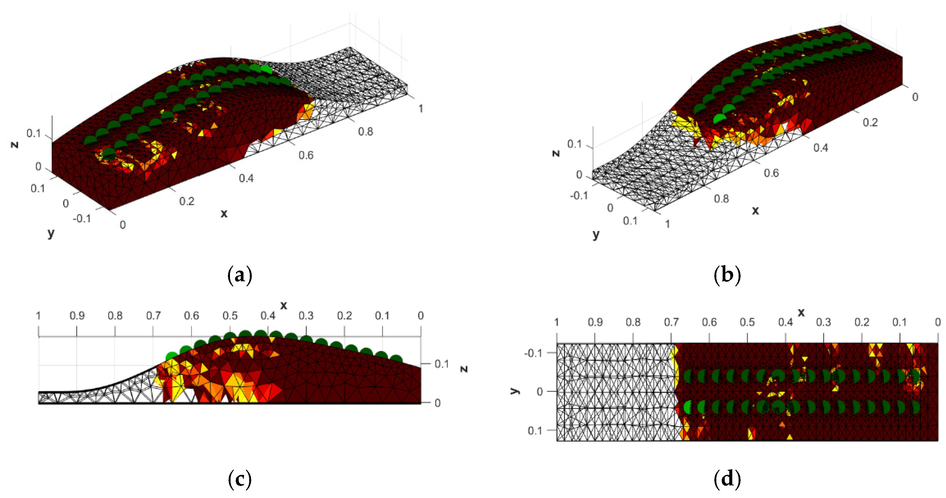
3.3. Image Reconstruction for Model III

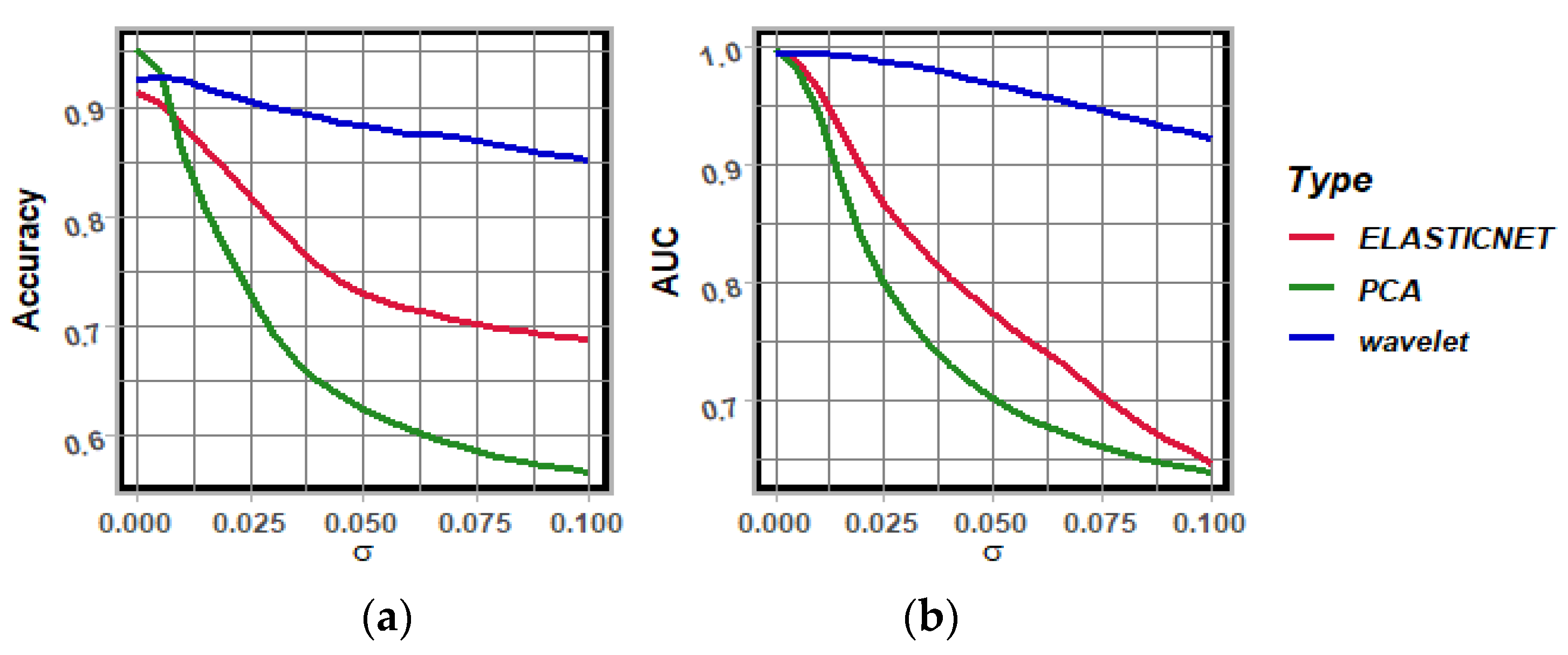
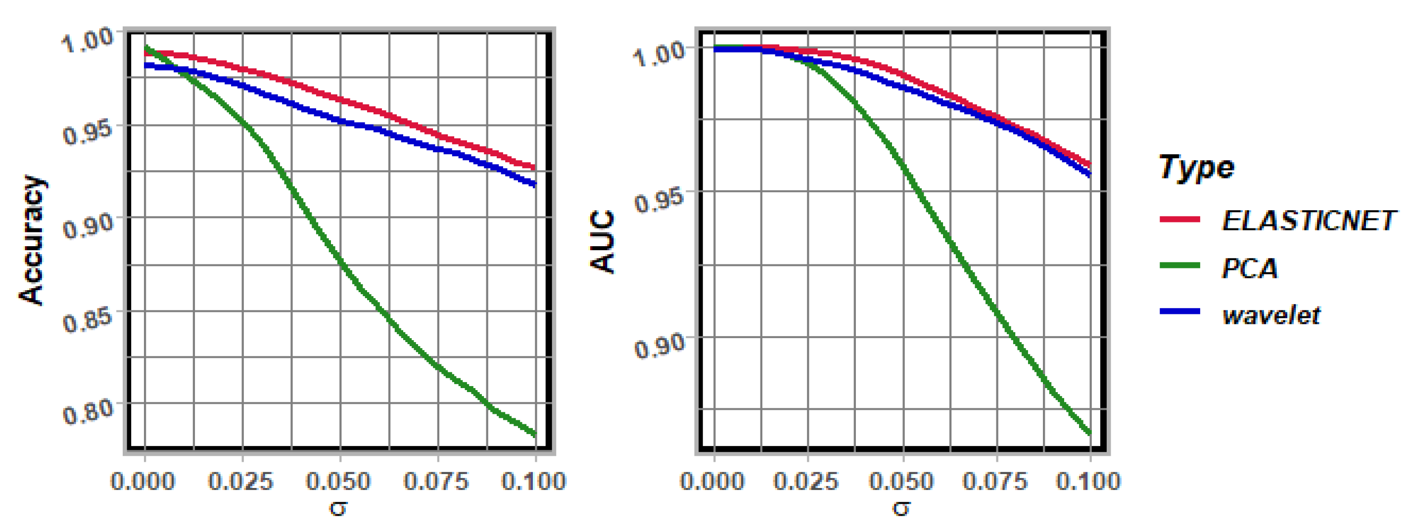
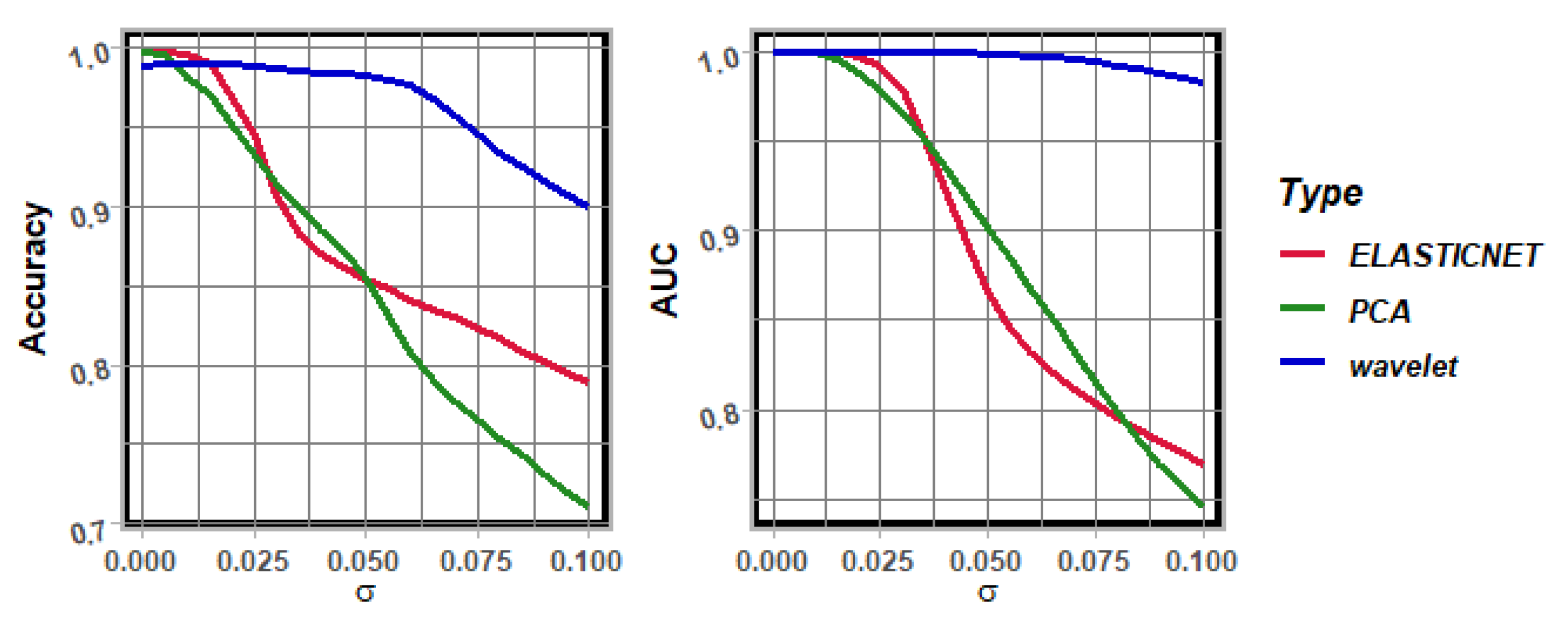
Figure 33 shows a numerical model of a dike with electrodes placed on its surface in one row. Model I consists of 2 × 16 electrodes, 3844 nodes, 16,240 finite elements and multi-sensors. Figure 34, Figure 35, Figure 36, Figure 37, Figure 38 and Figure 39 summary the image reconstruction for Model III. Three image reconstruction models were tested, and are shown in Figure 34, Figure 36 and Figure 38, with different variations of water infiltration. The data in

Table 9. The basic characteristics of the reconstruction for model III—example 7.

	Elasticnet	PCA	Wave
Sensitivity	0.9993290	1.0000000	0.9793659
Specificity	0.9878393	0.9936764	0.9857963
Pos Pred Value	0.9794476	0.9892134	0.9756016
Neg Pred Value	0.9996062	1.0000000	0.9880070
Precision	0.9794476	0.9892134	0.9756016
Recall	0.9993290	1.0000000	0.9793659
F1	0.9892884	0.9945775	0.9774801
Prevalence	0.3670567	0.3670567	0.3670567
Detection Rate	0.3668103	0.3670567	0.3594828
Detection Prevalence	0.3745074	0.3710591	0.3684729
Balanced Accuracy	0.9935841	0.9968382	0.9825811
AUC	0.9998543	0.9999899	0.9992118

,

Table 10. The basic characteristics of the reconstruction for model III—example 8.

	Elasticnet	PCA	Wave
Sensitivity	0.9673838	0.9871617	0.9906315
Specificity	0.9870179	0.9842497	0.9722222
Pos Pred Value	0.9761905	0.9718190	0.9515081
Neg Pred Value	0.9821429	0.9928743	0.9947260
Precision	0.9761905	0.9718190	0.9515081
Recall	0.9673838	0.9871617	0.9906315
F1	0.9717672	0.9794302	0.9706757
Prevalence	0.3549261	0.3549261	0.3549261
Detection Rate	0.3433498	0.3503695	0.3516010
Detection Prevalence	0.3517241	0.3605296	0.3695197
Balanced Accuracy	0.9772009	0.9857057	0.9814269
AUC	0.9989309	0.9994747	0.9992595

and

Table 11. The basic characteristics of the reconstruction for model III—example 9.

	Elasticnet	PCA	Wave
Sensitivity	0.9981336	0.9960237	0.9982959
Specificity	0.8562676	0.9793209	0.8593311
Pos Pred Value	0.9562311	0.9934439	0.9571306
Neg Pred Value	0.9931892	0.9873874	0.9937998
Precision	0.9562311	0.9934439	0.9571306
Recall	0.9981336	0.9960237	0.9982959
F1	0.9767331	0.9947322	0.9772799
Prevalence	0.7588054	0.7588054	0.7588054
Detection Rate	0.7573892	0.7557882	0.7575123
Detection Prevalence	0.7920567	0.7607759	0.7914409
Balanced Accuracy	0.9272006	0.9876723	0.9288135
AUC	0.9981009	0.9995930	0.9978249

show the results of the exact reconstructions shown in Figure 34, Figure 36 and Figure 38. The accuracy of the ROC statistical model for Model III is evaluated in Figure 35, Figure 37 and Figure 39.

The analysis of the accuracy of the reconstruction of the disturbances arising in the measurement obtained from the signals of the depth sensors is shown in Figure 38.

In order to verify the numerical studies performed, a laboratory model with depth sensors was constructed (Figure 39). Then, the object was flooded with water. The image reconstruction results for machine learning methods are shown in Figure 40. Laboratory model with depth sensors for 32 measuring electrodes and the reconstruction based on real measurements were presented in Figure 41 and Figure 42.

4. Discussion

This paper presented a monitoring system for flood embankments, and measurement models for water leakage were prepared. The designed models were equipped with different variants of sensors. In the first two models, point electrodes were used, while in the third model, multi-sensor electrodes were prepared. This solution directly measures specific electrical quantities and their corresponding analysis in the monitoring and damaging of flood embankments. Furthermore, machine learning algorithms were used and appropriately implemented for image reconstruction. Moreover, this is a novel approach in the application of machine learning algorithms, as other methods cannot estimate seepage in the entire volume of the object.

In this study, three flood embankment models with point and multi-sensor electrodes were implemented. The different sensors were evenly distributed along the edge of the object and inside it, depending on the model tested and the number of electrodes applied. The image reconstruction results show the great potential of the proposed solution for leakage analysis. Logistic regression with an elastic net, logistic regression with PCA, and wavelet decomposition methods solved the inverse problem. Furthermore, the solution presented works very quickly (reconstruction takes fractions of a second) and with high accuracy.

The main objectives of the research were to improve the resolution of the reconstructed image and increase the sensitivity of the monitoring system to changes occurring inside the floodbank. Thus, knowing the voltage values, the conductivity of the soil between the electrodes can be calculated. A separate algorithm generates each point of the output image. Due to the volume of data and equations to learn, the implementation of the assumptions required cloud computing. It is worth noting that the primary goal of EIT tomography is not to perfectly estimate the conductivity of the finite elements defined on the section mesh. The real goal is a faithful and accurate representation of the interior of the test object. Thus, it does not matter if the colours in the drawing correspond to the actual conductivity of the finite elements hidden inside the dike. However, it is important that the inclusions can be identified, regardless of their number, shape, and location.

By analysing Table 3, Table 4, Table 5, Table 6, Table 7, Table 8, Table 9, Table 10 and Table 11, it can be observed that the images obtained represent the models and examples studied with high accuracy. From the tables, one can read the error values of the reconstructed images relative to their models. It can be noticed that the majority of the pixels on the mesh do not include any errors. The comparative analysis of the three studied methods in the image reconstruction shows the high accuracy of each algorithm. Depending on the model and example studied, each method proves more or less accurate.

For the model shown in Figure 43, the correlation between the 96 features was determined (the signal contains 96 measurements between the electrodes). As we look at the heat map for these 96 features, we see that they are correlated.

On the other hand, by performing a PCA analysis (see Figure 44 and

Table 12. Contributions of the components in explaining the variability of the features.

	Percentage of Variance	Cumulative Percentage of Variance
comp 1	75.88	75.88
comp 2	10.48	86.37
comp 3	4.87	91.24
comp 4	3.26	94.50
comp 5	1.30	95.80
comp 6	1.19	96.99
comp 7	0.60	97.58
comp 8	0.50	98.09
comp 9	0.30	98.39
comp 10	0.25	98.64

), we can see that five principal components explain 95% of the variation in the traits, and 10 principal components explain 98.6% of the variation in the traits.

In Figure 44, we see an exponential relationship between the contribution to the explanation of feature variance and the principal component number. The use of an elastic net shows that the finite element conductivity is best explained by measurements read from the electrodes closest to the finite element. Reconstructions obtained using logistic regression with an elastic net, PCA decomposition, and wavelet preprocessing were compared with results obtained using deterministic methods involving the variance reduction of regression models, such as total variation and Tikhonov regularization. The values obtained by logistic regression are in the interval [0, 1], so additionally, a linear transformation was performed where the value “0” corresponds to the reference value of the conductivity, while the value “1” corresponds to the inclusion conductivity. Figure 45 shows the pattern and reconstruction results.

The following measures were used to compare the reconstruction results with the standard: the total sum of squares (TSS), mean squared error (MSE), mean absolute error (MAE) and mean absolute percentage error (MAPE). The results of the comparisons are presented in the table below (

Table 13. Matrix of the prediction accuracy measures.

Methods	TSS	MSE	MAE	MAPE
Logistic regression with Elasticnet	788.349	0.049	0.083	4.201
Logistic regression with PCA	425.786	0.026	0.028	1.705
Logistic regression with wavelet	611.791	0.038	0.049	3.453
Tikhonov regularization	23,993.577	1.477	0.689	28.752
Total variation	7051.689	0.434	0.379	24.462

).

For the model presented here, the use of logistic regression techniques improved the quality of the reconstruction. By comparing the results from the table, we can see that for the logistic regression models, the mean square error (MSE) for each finite element does not exceed 0.05, while in the case of the use of Tikhonov regularization alone, this error is almost 30 times higher, and in the case of the total variation technique it is almost eight times higher. By comparing the MAE and MAPE (mean absolute error and mean percentage error), we can see that they are several times smaller than for the Tikhonov regularization and the total variation for logistic regression. The results of the comparisons are shown in the table below (Figure 46).

For the shaft model (where the electrodes are placed only on one side of the viewing objection), by comparing the results from the table, we can see that the quality of reconstructions obtained by logistic regression with PCA and wavelet, and by total variation are quite good. In contrast, the reconstructions by logistic regression with an elastic net and by Tikhonov regularization are slightly worse. Furthermore, for the case of logistic regression with PCA, the mean absolute error (MAE) is even lower than for total variation, while the mean squared error (MSE) and mean percentage error (MAPE) for the total variation technique is smaller than that for logistic regression with PCA (

Table 14. Matrix of the prediction accuracy measures.

Methods	TSS	MSE	MAE	MAPE
Logistic regression with Elasticnet	3848.001	0.392	0.288	19.663
Logistic regression with PCA	2255.186	0.230	0.140	10.586
Logistic regression with wavelet	4683.420	0.478	0.262	11.266
Tikhonov regularization	6118.022	0.624	0.353	17.557
Total variation	1852.541	0.189	0.158	9.344

).

Logistic regression with wavelet preprocessing is the most robust to noise, while logistic regression with PCA decomposition is the most sensitive to the real model.

5. Conclusions

The main purpose of the work was to develop image reconstruction algorithms for leakage analysis in various flood embankment models. The presented solution enables a fairly accurate assessment of the properties of the tested objects, and gives promising results. Algorithms based on logistic regression machine learning methods with an elastic net regularisation, PCA and wave preprocessing were used to calculate the leakage in order to obtain more accurate and stable image reconstruction, leading to a solution of the inverse problem in EIT. A measurement system and three models for the reconstruction of tomographic images with point and depth electrodes were developed in a laboratory study. Using a system of multiple separate algorithms running simultaneously to image the cross-section of a flood barrier allows the generation of accurate representations of specific patterns. The quality of this data is adequate to identify leakage over time correctly.

Furthermore, given the ability to take measurements at fixed time intervals, it is easy to determine the velocity of the leakage propagation. This information enables an accurate diagnosis to help determine the reliability of the dam. With this information, the tomographic system can plan appropriate actions before dam failure.

The approach presented was used to identify areas of high-probability inclusions, so logistic regression was used for this purpose. The main problem in EIT is the problem of the collinearity of features (measurements from the electrodes). In order to improve the quality of the classifier, additional methods were applied. Using deterministic methods, the conductivity distribution was determined and compared with the machine learning methods. The use of logistic regression for each finite element makes it possible to determine (extract) the inclusion regions. In the case of signals from electrodes without interference, the analysis of the reconstruction results using logistic regression with an elastic net and PCA is slightly better than logistic regression with wavelet preprocessing. However, when additional disturbances are introduced to the electrodes, recognising the inclusion in the visual area is better for logistic regression with wavelet preprocessing.

The study shows that the wavelet technique is a competitive approach compared to PCA and elastic net. Additionally, the reconstructions are more robust to perturbations arising during measurements. Many wavelets are known in the literature. Further studies will investigate the quality of reconstructions using different wavelets.

References

1. Forson, A.; Comas, X.; Whitman, D. Integration of electrical resistivity imaging and ground penetrating radar to investigate solution features in the Biscayne Aquifer. J. Hydrol. 2014, 515, 129–138. [Google Scholar] [CrossRef]
2. De Donno, G.; Di Giambattista, L.; Orlando, L. High-resolution investigation of masonry samples through GPR and electrical resistivity tomography. Constr. Build. Mater. 2017, 154, 1234–1249. [Google Scholar] [CrossRef]
3. Bukowska-Belniak, B.; Borecka, A.; Leśniak, A. The continuous thermal imaging of the flood embankment to identify location of the leaks. In Proceedings of the 14th Quantitative InfraRed Thermography Conference, Berlin, Germany, 25–29 June 2018. [Google Scholar]
4. Crawford, M.M.; Bryson, L.S.; Woolery, E.W.; Wang, Z. Using 2-D electrical resistivity imaging for joint geophysical and geotechnical characterization of shallow landslides. J. Appl. Geophys. 2018, 157, 37–46. [Google Scholar] [CrossRef]
5. Lesparre, N.; Nguyen, F.; Kemna, A.; Robert, T.; Hermans, T.; Daoudi, M.; Flores-Orozco, A. A new approach for time-lapse data weighting in electrical resistivity tomography. Geophysics 2017, 82, E325–E333. [Google Scholar] [CrossRef]
6. Hojat, A.; Ferrario, M.; Arosio, D.; Brunero, M.; Ivanov, V.; Longoni, L.; Madaschi, A.; Papini, M.; Tresoldi, G.; Zanzi, L. Laboratory Studies Using Electrical Resistivity Tomography and Fiber Optic Techniques to Detect Seepage Zones in River Embankments. Geosciences 2021, 11, 69. [Google Scholar] [CrossRef]
7. Ghafoori, Y.; Vidmar, A.; Říha, J.; Kryžanowski, A. A Review of Measurement Calibration and Interpretation for Seepage Monitoring by Optical Fiber Distributed Temperature Sensors. Sensors 2020, 20, 5696. [Google Scholar] [CrossRef]
8. Bossi, G.; Bersan, S.; Cola, S.; Schenato, L.; De Polo, F.; Menegazzo, C.; Boaga, J.; Cassiani, G.; Donini, F.; Simonini, P. Multidisciplinary analysis and modelling of a river embankment affected by piping. In European Working Group on Internal Erosion; Springer: Cham, Switzerland, 2018; pp. 234–244. [Google Scholar]
9. Schenato, L. A Review of Distributed Fibre Optic Sensors for Geo-Hydrological Applications. Appl. Sci. 2017, 7, 896. [Google Scholar] [CrossRef]
10. Bersan, S.; Koelewijn, A.R.; Simonini, P. Effectiveness of distributed temperature measurements for early detection of piping in river embankments. Hydrol. Earth Syst. Sci. Discuss. 2018, 22, 1491–1508. [Google Scholar] [CrossRef] [Green Version]
11. Habel, W.R.; Krebber, K. Fiber-optic sensor applications in civil and geotechnical engineering. Photonics Sens. 2011, 1, 268–280. [Google Scholar] [CrossRef] [Green Version]
12. Ghafoori, Y.; Maček, M.; Vidmar, A.; Říha, J.; Kryžanowski, A. Analysis of Seepage in a Laboratory Scaled Model Using Passive Optical Fiber Distributed Temperature Sensor. Water 2020, 12, 367. [Google Scholar] [CrossRef] [Green Version]
13. Rymarczyk, T. Using electrical impedance tomography to monitoring flood banks. Int. J. Appl. Electromagn. Mech. 2014, 45, 489–494. [Google Scholar] [CrossRef]
14. Jones, G.; Sentenac, P.; Zielinski, M. Desiccation cracking detection using 2-D and 3-D Electrical Resistivity Tomography: Validation on a flood embankment. J. Appl. Geophys. 2014, 106, 196–211. [Google Scholar] [CrossRef] [Green Version]
15. Michta, E.; Szulim, R.; Sojka-Piotrowska, A.; Piotrowski, K. IoT-based flood embankments monitoring system. In Photonics Applications in Astronomy, Communications, Industry, and High Energy Physics Experiments 2017; SPIE: Bellingham, WA, USA, 2017; Volume 10445, p. 104455Y. [Google Scholar] [CrossRef]
16. Sekuła, K.; Połeć, M.; Borecka, A. Innovative solutions in monitoring systems in flood protection. E3S Web Conf. Water Wastewater Energy Smart Cities 2018, 30, 01005. [Google Scholar] [CrossRef] [Green Version]
17. Rymarczyk, T.; Kozłowski, E.; Kłosowski, G. Electrical impedance tomography in 3D flood embankments testing—Elastic net approach. Trans. Inst. Meas. Control 2020, 42, 680–690. [Google Scholar] [CrossRef]
18. Rymarczyk, T.; Kłosowski, G. Application of neural reconstruction of tomographic images in the problem of reliability of flood protection facilities. Eksploat. Niezawodn.-Maint. Reliab. 2018, 20, 425–434. [Google Scholar] [CrossRef]
19. Daniewski, K.; Kosicka, E.; Mazurkiewicz, D. Analysis of the correctness of determination of the effectiveness of maintenance service actions. Manag. Prod. Eng. Rev. 2018, 9, 20–25. [Google Scholar]
20. Korzeniewska, E.; Sekulska-Nalewajko, J.; Gocawski, J.; Droż, T.; Kiebasa, P. Analysis of changes in fruit tissue after the pulsed electric field treatment using optical coherence tomography. EPJ Appl. Phys. 2020, 91, 30902. [Google Scholar] [CrossRef]
21. Dusek, J.; Mikulka, J. Measurement-Based Domain Parameter Optimization in Electrical Impedance Tomography Imaging. Sensors 2021, 21, 2507. [Google Scholar] [CrossRef]
22. Mosorov, V.; Rybak, G.; Sankowski, D. Plug Regime Flow Velocity Measurement Problem Based on Correlability Notion and Twin Plane Electrical Capacitance Tomography: Use Case. Sensors 2021, 21, 2189. [Google Scholar] [CrossRef]
23. Szczesny, A.; Korzeniewska, E. Selection of the method for the earthing resistance measurement. Przegląd Elektrotech. 2018, 94, 178–181. [Google Scholar]
24. Liu, S.; Huang, Y.; Wu, H.; Tan, C.; Jia, J. Efficient Multitask Structure-Aware Sparse Bayesian Learning for Frequency-Difference Electrical Impedance Tomography. IEEE Trans. Ind. Inform. 2021, 17, 463–472. [Google Scholar] [CrossRef] [Green Version]
25. Wajman, R.; Banasiak, R.; Babout, L. On the Use of a Rotatable ECT Sensor to Investigate Dense Phase Flow: A Feasibility Study. Sensors 2020, 20, 4854. [Google Scholar] [CrossRef] [PubMed]
26. Zou, H.; Hastie, T. Regularization and variable selection via the elastic net. J. R. Stat. Soc. Ser. B 2005, 67, 301–320. [Google Scholar] [CrossRef] [Green Version]
27. Mevik, B.-H.; Wehrens, R. The pls Package: Principal Component and Partial Least Squares Regression in R. J. Stat. Softw. 2007, 18, 1–23. [Google Scholar] [CrossRef] [Green Version]
28. Daubechies, I. Orthonormal Bases of Compactly Supported Wavelets. Commun. Pure Appl. Math. 1992, 41, 909–996. [Google Scholar] [CrossRef] [Green Version]
29. Holder, D.S. Introduction to Biomedical Electrical Impedance Tomography Electrical Impedance Tomography Methods; History and Applications Bristol, Institute of Physics: Bristol, UK, 2005. [Google Scholar]
30. Rymarczyk, T. New methods to determine moisture areas by electrical impedance tomography. Int. J. Appl. Electromagn. Mech. 2016, 52, 79–87. [Google Scholar] [CrossRef]
31. Adler, A.; Lionheart, W. Uses and abuses of EIDORS: An extensible software base for EIT. Physiol. Meas. 2006, 27, S25–S42. [Google Scholar] [CrossRef] [Green Version]
32. Dušek, J.; Hladký, D.; Mikulka, J. Electrical Impedance Tomography Methods and Algorithms Processed with a GPU. In Proceedings of the 2017 Progress in Electromagnetics Research Symposium—Spring (PIERS), St. Petersburg, Russia, 22–25 May 2017; pp. 1710–1714. [Google Scholar]
33. Kozłowski, E.; Mazurkiewicz, D.; Żabiński, T.; Prucnal, S.; Sęp, J. Assessment model of cutting tool condition for real-time supervision system. Eksploat. Niezawodn.-Maint. Reliab. 2019, 21, 679–685. [Google Scholar] [CrossRef]
34. Rymarczyk, T.; Kłosowski, G.; Hoła, A.; Sikora, J.; Wołowiec, T.; Tchórzewski, P.; Skowron, S. Comparison of Machine Learning Methods in Electrical Tomography for Detecting Moisture in Building Walls. Energies 2021, 14, 2777. [Google Scholar] [CrossRef]
35. Rymarczyk, T.; Nita, P.; Vejar, A.; Woś, M.; Stefaniak, B.; Adamkiewicz, P. Wearable mobile measuring device based on electrical tomography. Przegląd Elektrotech. 2019, 95, 211–214. [Google Scholar]
36. Chen, B.; Abascal, J.F.P.J.; Soleimani, M. Extended Joint Sparsity Reconstruction for Spatial and Temporal ERT Imaging. Sensors 2018, 18, 4014. [Google Scholar] [CrossRef] [Green Version]
37. Rymarczyk, T.; Kłosowski, G.; Tchórzewski, P.; Cieplak, T.; Kozłowski, E. Area monitoring using the ERT method with multisensor electrodes. Przegląd Elektrotech. 2019, 95, 153–156. [Google Scholar] [CrossRef] [Green Version]
38. Rybak, G.; Strzecha, K. Short-Time Fourier Transform Based on Metaprogramming and the Stockham Optimization Method. Sensors 2021, 21, 4123. [Google Scholar] [CrossRef] [PubMed]
39. Voss, A.; Pour-Ghaz, M.; Vauhkonen, M.; Seppänen, A. Retrieval of the saturated hydraulic conductivity of cement-based materials using electrical capacitance tomography. Cem. Concr. Compos. 2020, 112, 103639. [Google Scholar] [CrossRef]
40. Shi, X.; Tan, C.; Dong, F.; dos Santos, E.N.; da Silva, M.J. Conductance Sensors for Multiphase Flow Measurement: A Review. IEEE Sens. J. 2021, 21, 12913–12925. [Google Scholar] [CrossRef]
41. Midura, M.; Wróblewski, P.; Wanta, D.; Domański, G.; Stosio, M.; Kryszyn, J.; Smolik, W.T. The system for complex magnetic susceptibility measurement of nanoparticles with 3d printed carcass for integrated receive coils. Inform. Autom. Pomiary Gospod. Ochr. Sr. 2021, 11, 4–9. [Google Scholar] [CrossRef]
42. Sekulska-Nalewajko, J.; Gocławski, J.; Korzeniewska, E. A method for the assessment of textile pilling tendency using optical coherence tomography. Sensors 2020, 20, 3687. [Google Scholar] [CrossRef]
43. Rzasa, M.; Czapla-Nielacna, B. Analysis of the Influence of the Vortex Shedder Shape on the Metrological Properties of the Vortex Flow Meter. Sensors 2021, 21, 4697. [Google Scholar] [CrossRef]
44. Fiala, P.; Bartušek, K.; Dědková, J.; Dohnal, P. EMG field analysis in dynamic microscopic/nanoscopic models of matter. Inform. Autom. Pomiary Gospod. Ochr. Sr. 2019, 9, 4–10. [Google Scholar] [CrossRef]
45. Kłosowski, G.; Rymarczyk, T.; Wójcik, D.; Skowron, S.; Adamkiewicz, P. The Use of Time-Frequency Moments as Inputs of LSTM Network for ECG Signal Classification. Electronics 2020, 9, 1452. [Google Scholar] [CrossRef]
46. Fawcett, T. An introduction to ROC analysis. Pattern Recognit. Lett. 2006, 27, 861–874. [Google Scholar] [CrossRef]
47. Hand, D.J.; Till, R.J. A simple generalisation of the area under the roc curve for multiple class classification problems. Mach. Learn. 2001, 45, 171–186. [Google Scholar] [CrossRef]
48. Rymarczyk, T.; Kozłowski, E.; Kłosowski, G.; Niderla, K. Logistic Regression for Machine Learning in Process Tomography. Sensors 2019, 19, 3400. [Google Scholar] [CrossRef] [Green Version]
49. Wehrens, R. Chemometrics with R. Multivariate Data Analysis in the Natural Science and Life Sciences; Springer: New York, NY, USA, 2011. [Google Scholar]
50. Hastie, T.; Tibshirani, R.; Friedman, J. The Elements of Statistical Learning: Data Mining, Inference, and Prediction; Springer Science & Business Media: New York, NY, USA, 2009. [Google Scholar]
51. James, G.; Witten, D.; Hastie, T.; Tibshirani, R. An Introduction to Statistical Learning with Applications in R; Springer: New York, NY, USA, 2013. [Google Scholar]
52. Tibshirani, R. Regression Shrinkage and Selection Via the Lasso. J. R. Stat. Soc. Ser. B 1996, 58, 267–288. [Google Scholar] [CrossRef]
53. Friedman, J.; Tibshirani, R.; Hastie, T. Regularization paths for generalised linear models via coordinate descent. J. Stat. Softw. 2010, 33, 1–22. [Google Scholar] [CrossRef] [PubMed] [Green Version]
54. Yan, X.; Su, X.G. Linear Regression Analysis; World Scientific Publishing Company: London, UK, 2009. [Google Scholar]
55. Percival, D.B.; Walden, A. Wavelet Methods for Time Series Analysis; Cambridge University Press: Cambridge, UK, 2000; Volume 4. [Google Scholar]
56. Walnut, D.F. An Introduction to Wavelet Analysis; Springer Nature: Basingstoke, UK, 2004. [Google Scholar]
Figure 1. Monitoring system based on electrical tomography.
Energies 14 08081 g001
Figure 2. Block diagram of the tomograph.
Energies 14 08081 g002
Figure 3. Electric tomograph: (a) measuring unit, (b) communication and control unit, (c) inside view, and (d) panel.
Energies 14 08081 g003
Figure 4. Laboratory system with measuring electrodes during measurements with an electrical tomograph.
Energies 14 08081 g004
Figure 5. Laboratory model with two multi-sensor electrodes during electrical tomography measurements.
Energies 14 08081 g005
Figure 6. Learning process.
Energies 14 08081 g006
Figure 7. Reconstruction process.
Energies 14 08081 g007
Figure 8. Numerical model I of the flood embankment with 16 measuring electrodes.
Energies 14 08081 g008
Figure 9. Model I flood embankment with 16 electrodes, with water infiltration on the left side. Example 1: (a) the pattern, (b) logistic regression with an elastic net, (c) logistic regression with PCA decomposition, and (d) logistic regression with wavelet decomposition.
Energies 14 08081 g009
Figure 10. ROC analysis for model I—example 1.
Energies 14 08081 g010
Figure 11. Model I flood embankment with 16 electrodes, with water infiltration on the right side. Example 2: (a) pattern, (b) logistic regression with an elastic net, (c) logistic regression with PCA decomposition, and (d) logistic regression with wavelet decomposition.
Energies 14 08081 g011
Figure 12. ROC analysis for model I—example 2.
Energies 14 08081 g012
Figure 13. Model I flood embankment with 16 electrodes, with water infiltration throughout the area. Example 3: (a) pattern, (b) logistic regression with an elastic net, (c) logistic regression with PCA decomposition, and (d) logistic regression with wavelet decomposition.
Energies 14 08081 g013
Figure 14. ROC analysis for model I—example 3.
Energies 14 08081 g014
Figure 15. Influence of disturbances of the reconstruction quality-model I: (a) Accuracy, (b) AUC.
Energies 14 08081 g015
Figure 16. A laboratory model of the flooded embankment with 16 measuring sensors.
Energies 14 08081 g016
Figure 17. Reconstruction based on real measurements-model I: (a) logistic regression with an elastic net, (b) logistic regression with PCA decomposition, (c) logistic regression with wavelet decomposition.
Energies 14 08081 g017
Figure 18. Reconstruction based on real measurement - regression with an elastic net and different projections for model I-views: (a) front, (b) back, (c) side, (d) top.
Energies 14 08081 g018
Figure 19. Reconstruction based on real measurements—regression with PCA and different projections for model I-views: (a) front, (b) back, (c) side, (d) top.
Energies 14 08081 g019
Figure 20. Reconstruction based on real measurements—regression with different wavelet projections for model I-views: (a) front, (b) back, (c) side, (d) top.
Energies 14 08081 g020
Figure 21. Numerical model II of flood embankments with 32 measuring electrodes.
Energies 14 08081 g021
Figure 22. Model II flood embankment with 32 electrodes, with water infiltration on the left side. Example 4: (a) pattern, (b) logistic regression with an elastic net, (c) logistic regression with PCA decomposition, and (d) logistic regression with wavelet decomposition.
Energies 14 08081 g022
Figure 23. ROC analysis for model II—example 4.
Energies 14 08081 g023
Figure 24. Model II flood embankment with 32 electrodes, with water infiltration throughout the area. Example 5: (a) pattern, (b) logistic regression with an elastic net, (c) logistic regression with PCA decomposition, and (d) logistic regression with wavelet decomposition.
Energies 14 08081 g024
Figure 25. ROC analysis for model II—example 5.
Energies 14 08081 g025
Figure 26. Model II flood embankment with 32 electrodes, with water infiltration on the right side. Example 6: (a) pattern, (b) logistic regression with an elastic net, (c) logistic regression with PCA decomposition, and (d) logistic regression with wavelet decomposition.
Energies 14 08081 g026
Figure 27. ROC analysis for model II—example 6.
Energies 14 08081 g027
Figure 28. Influence of disturbances on the reconstruction quality—model II.
Energies 14 08081 g028
Figure 29. Reconstruction based on real measurements—model II: (a) logistic regression with an elastic net, (b) logistic regression with PCA decomposition, and (c) logistic regression with wavelet decomposition.
Energies 14 08081 g029
Figure 30. Reconstruction based on real measurements—regression with an elastic net and different projections for model II-views: (a) front, (b) back, (c) side, (d) top.
Energies 14 08081 g030
Figure 31. Reconstruction based on real measurements—regression with PCA and different projections for model II-views: (a) front, (b) back, (c) side, (d) top.
Energies 14 08081 g031
Figure 32. Reconstruction based on real measurements—regression with different wavelet projections for model II-views: (a) front, (b) back, (c) side, (d) top.
Energies 14 08081 g032
Figure 33. Numerical model III of flood embankments with depth sensors.
Energies 14 08081 g033
Figure 34. Model III with depth sensors, with water infiltration inside the area. Example 7: (a) pattern, (b) logistic regression with an elastic net, (c) logistic regression with PCA decomposition, (d) logistic regression with wavelet decomposition.
Energies 14 08081 g034
Figure 35. ROC analysis for model III—example 7.
Energies 14 08081 g035
Figure 36. Model III with depth sensors, with water infiltration on the right side. Example 8: (a) pattern, (b) logistic regression with an elastic net, (c) logistic regression with PCA decomposition (d) logistic regression with wavelet decomposition.
Energies 14 08081 g036
Figure 37. ROC analysis for model III—example 8.
Energies 14 08081 g037
Figure 38. Model III with depth sensors, with water infiltration at the top. Example 9: (a) pattern, (b) logistic regression with an elastic net, (c) logistic regression with PCA decomposition, and (d) logistic regression with wavelet decomposition.
Energies 14 08081 g038
Figure 39. ROC analysis for model III—example 9.
Energies 14 08081 g039
Figure 40. Influence of disturbances into the reconstruction quality—model III.
Energies 14 08081 g040
Figure 41. Laboratory model with depth sensors-32 measuring electrodes.
Energies 14 08081 g041
Figure 42. Reconstruction based on real measurements—model III: (a) logistic regression with an elastic net, (b) logistic regression with PCA decomposition, and (c) logistic regression with wavelet decomposition.
Energies 14 08081 g042
Figure 43. Heatmap of the correlation between the attributes.
Energies 14 08081 g043
Figure 44. The exponential relationship between the contribution to the explanation of feature variance and the principal component number.
Energies 14 08081 g044
Figure 45. Pattern and reconstruction results obtained by the machine learning and deterministic methods for the model with depth electrodes.
Energies 14 08081 g045
Figure 46. Pattern and reconstruction results obtained by machine learning and deterministic methods-model with surface electrodes.
Energies 14 08081 g046