Logistic Regression with Wave Preprocessing to Solve Inverse Problem in Industrial Tomography for Technological Process Control

Abstract

The research presented here concerns the analysis and selection of logistic regression with wave preprocessing to solve the inverse problem in industrial tomography. The presented application includes a specialized device for tomographic measurements and dedicated algorithms for image reconstruction. The subject of the research was a model of a tank filled with tap water and specific inclusions. The research mainly targeted the study of developing and comparing models and methods for data reconstruction and analysis. The application allows choosing the appropriate method of image reconstruction, knowing the specifics of the solution. The novelty of the presented solution is the use of original machine learning algorithms to implement electrical impedance tomography. One of the features of the presented solution was the use of many individually trained subsystems, each of which produces a unique pixel of the final image. The methods were trained on data sets generated by computer simulation and based on actual laboratory measurements. Conductivity values for individual pixels are the result of the reconstruction of vector images within the tested object. By comparing the results of image reconstruction, the most efficient methods were identified.

1. Introduction

Tomography is a method of examining the interior of objects based on measurements taken at the edge of that object. It is a non-invasive method, which can be used to obtain a cross-section of the element—providing 2D images—or spatially—providing 3D images. The device for taking measurements is called a tomograph, and the image obtained from the measurements is called a tomogram. Mathematical operations and techniques called tomographic reconstruction are used to obtain the image. Different physical phenomena are used depending on the type of object under study. The carriers may be ultrasound, electron beams, electric currents or magnetic fields. Depending on the specificity of a given tomographic technique, we can observe both advantages and disadvantages in the areas of accuracy, frequency or resolution of reconstructed images. Familiarization with the characteristics of individual tomographic techniques allows for the proper selection of an image reconstruction method. Tomographic imaging offers a unique opportunity to study the complexity of a structure without interfering with the object [1,2]. There is an increasing demand for information about the behavior of the internal flows in process equipment. This information should be obtained in a non-invasive way with tomographic instrumentation. Typical measuring equipment is usually inadequate for the complicated process internal conditions, and sometimes its existence can interfere with the process. Industrial tomography is used to control measurement data. The facility to be monitored is a tomographically instrumented part of a manufacturing plant, where a device non-invasively collects data using excitatory electrical potentials on its surface. The instrument sends the raw data to a cloud computing system where an inverse problem (image reconstruction) is resolved. As a result, the state of the monitored object is classified using a machine learning algorithm. Figure 1 presents a general scheme of how the system works.

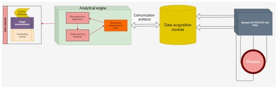
Figure 1. Model of a tomographic sensor platform with an analytical system.

The presented solution enables tomographic sensor-based process control, Big Data analysis, multidimensional industrial process control, advanced human–machine interfaces and knowledge-based process monitoring. Sensor technology is mostly related to electrical tomography (ET) [3,4], which includes capacitive tomography (ECT) [5,6,7,8,9] and electrical resistive tomography (ERT) [10,11]. This solution allows the image to be reconstructed as the conductivity or permittivity distribution of the reservoir under study by measuring its boundary. Another method is optical coherence tomography (OCT), which is an optical technique that allows non-invasive imaging of specimens [12], and ultrasound tomography (UST) [13,14], which is a technique that uses the information included in the ultrasound signal after it has passed through the test object.

Electrical impedance tomography (EIT) is a non-destructive method for creating image reconstructions in various application areas. It is suitable for real-time visualization and the analysis of the electrical conductivity distribution inside the analyzed object [15]. EIT is now a widely used tomographic imaging technique and applies to many areas of everyday life. This technique has found applications in fields such as medical diagnostics [4], industrial process monitoring [13] and geophysical surveys [16]. Mathematical reconstruction of conductivity in EIT involves solving a nonlinear and ill-posed inverse problem from noisy data [17,18]. The current development of EIT algorithms is heavily biased towards machine learning methods [3], and for such an operation, the data must be prepared appropriately. It raises the need to check whether particular algorithms are better than classical ones and can be used. Compared to other known imaging modalities, impedance tomography has many advantages. However, EIT reconstruction can be unstable, and the disadvantage of solving a backward problem should be mentioned. Furthermore, the sensitivity of EIT solutions to measurement, numerical and model errors implies the need to adapt model parameters to specific cases. At the same time, it should be remembered that most reconstruction methods in 2D space are equally effective in 3D.

The article presents an improved method of monitoring and optimizing processes in heterogeneous tank reactors in which specific reactions occur. The method used relates to electrical tomography, and the innovation is the original way of using a hybrid module system in parallel, combining logistic regression with wavelet preprocessing. The significant difference of the presented method over other non-invasive solutions is the reliability of disturbances arising during measurements and the accuracy of imaging reconstruction. In addition, our proposed method enables the appropriate selection of wavelet preprocessing algorithms for image pixels. It results in better reconstruction quality and higher image resolution.

This paper consists of four sections. The architecture of the designed system, industrial processes and application platform is presented in Section 2. Machine learning methods used for image reconstruction, numerical models, tomographic devices and laboratory measurement systems are also discussed. The results of the research work are presented in Section 3 in the form of image reconstructions for synthetic and measured data. Section 4 contains a discussion of the results obtained. Finally, Section 5 summarizes the research work.

2. Materials and Methods

This section shows the tomographic algorithms, system architecture, industrial tomography, measurement hardware, mathematical algorithms and measurement models used to reconstruct images from real and synthetic data.

The research used the SmartEIT 1.0 (Netrix S.A., Lublin, Poland), our electrical impedance tomograph and a specially prepared tank with EIT measuring electrodes.

For preliminary analyses of numerical models, Python 3.6 (Python Software Foundation, Amsterdam, Netherlands) with NumPy, math, SciPy libraries were used. MATLAB 2020B (MathWorks, Natick, MA, USA) and EIDORS (Ver: 3.9) (Sourceforge, San Diego, CA, USA) [19] were implemented to construct the case generator and visualize the reconstructions. Using R software (The R Foundation, Vienna, Austria), structural parameters were estimated, ROC analysis was performed and the relationship between FPR and TPR was graphically represented. For this purpose, the following packages (The R Foundation, Vienna, Austria) were used: R.matlab (Ver: 3.6.2), doParallel (Ver: 1.0.15), foreach (Ver: 1.5.0), glmnet (Ver: 4.0-2), caret (Ver: 6.0-86), pRoc (Ver: 1.16.2), ggplot2 (Ver: 3.3.1) and plotROC (Ver: 2.2.1).

2.1. Novelty of the Proposed Solution

The novelty of the solution presented in this paper is the combination of logistic regression with wavelet preprocessing methods to reconstruct the output image in industrial tomography. The approach proposed by the authors consists in implementing an algorithm with multiple trained subsystems. After converting the predictors to a binary grid, image reconstruction is generated. Voltage drop measurements are used as input data.

2.2. Industrial Electrical Tomography

Industrial tomography is used to analyze the technological processes inside the studied facility [2,5]. This approach allows for better real-time process control. Data concentration profiles, phases and chemicals can be studied using fast data acquisition and image reconstruction. The resulting data can be used to monitor process response, improve quality, yield and flow rate. The imaging technique presented here exploits the respective electrical properties of various kinds of substances. Electrical tomography can be divided into impedance tomography and capacitive tomography for dielectric systems. In this method, a current or voltage source is connected to the test object, the voltage distribution at the edge of the test object is measured using a measurement system. An image reconstruction algorithm processes the data collected from the above measurements. The reconstructed image is called a tomogram. It is worth noting that tomography is characterized by low image resolution. This has to do with the number of measurements, which is limited by the nonlinear current flow through the tested element but is also caused by the low sensitivity of the measured voltage waveforms, which depends on the conductivity changes inside the area.

2.3. Measuring Device

The device’s design is based on the idea of electrical tomography, which is based on the non-invasive measurement of voltage drops from electrodes on the tested object (Figure 2). Based on measurements of voltages on electrodes directly adjacent to a given medium, it is possible to determine impedance’s spatial distribution and thus visualize its internal structure. Due to the built-in microcomputer, it is possible to perform EIT measurements and view the reconstructions created on their basis. In addition, the device has a network interface that allows data transfer to an external server. The tomograph measures voltages by switching channels according to the polar method. First, EXC and GND outputs are connected to two opposite electrodes using multiplexers. The intensity of current flow is programmed to a set value. Then, the signal input is connected successively to the remaining electrodes, on which the voltage is measured to the GND electrode. After completing measurements, the measuring information is disconnected, the forcing electrodes are switched to the next pair and the cycle is repeated.

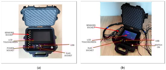
Figure 2. Photos showing the view of the SmartEIT scanner placed in the housing on the left (a) and the device connected to the probes and working—on the right (b).

Raspberry Pi sends and receives data from the measurement module using the SPI interface; Raspberry acts as Master by default, module as Slave. On receiving the command to start the sequence—the module starts measuring using the opposite method. Electrodes A and B force the flow of the alternating current of a sinusoidal waveform, where electrode A is connected via a multiplexer to the circuit of current intensity regulation, and electrode B is connected to GND of the circuit. The voltage is measured at successive electrodes to GND (Figure 3).

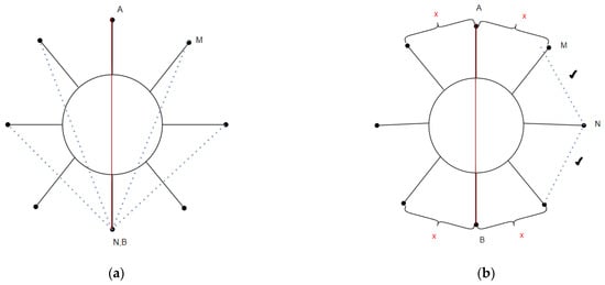
Figure 3. Acquisition method and measurement calculation (a), forcing electrodes A and B and measuring electrodes M and N (b).

2.4. Measurement System

The measurement system consists of a sensor tank; devices with a model for data transmission, collection and analysis are connected to a communication interface whose task is to read the signal from the selected sensor, process it into a coherent form and then send the read and processed data to the acquisition module (Figure 4). For this solution, an application was prepared with an algorithm for image reconstruction, which, using learning data obtained by computer simulation from real models, was trained to solve the inverse problem. Conductivity values of the individual pixels of the output vector allow the obtaining of images of the interior of the studied objects.

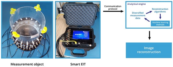
Figure 4. Measurement system with a model of data transmission, collection and analysis.

2.5. Algorithms and Methods

This section presents the descriptions of the used algorithms. Industrial tomography also belongs to electromagnetic field inverse problems. An inverse problem is an optimization, identification or synthesis process where parameters are determined by domain-specific information. Such problems do not have straightforward solutions and are ill-conditioned. Finite element methods solved the forward problem.

There are many optimization methods, using both deterministic and statistical algorithms [20,21,22,23,24,25,26,27]. Machine learning is a group of methods that is gaining increasing popularity in various types of tomography, including EIT. Applying the above methods requires the 2D cross-section of the test object to be divided into pixels by the finite element method. Typically, a single algorithm converts a set of measurements into the pixels that make up a tomographic image. It can also train separate models to convert measurements to a single image pixel. It then needs to train as many models as the resolution of the tomographic image. It was the approach taken in the research presented here.

For logistic regression, the implementation probability of the output variable is calculated relative to the corresponding category, where the inclusion probability is estimated [28,29,30,31,32,33]. Thus, the implementation of logistic regression enables the resolution of the imaging domain to be determined. When creating a reconstruction for EIT, we must estimate conductivity for each finite element. In the presented case, we calculate the probability that finite elements belong to inclusion. For this purpose, we define a logistic regression model [28] for each finite element. Thus, the reconstruction based on logistic regression must be defined as a set of logistic regressions corresponding to finite elements.

For each finite element, we define a learning set $D=\left\{\left(x_i,y_i\right):x_i\in {ℝ}^m, y_i\in \left\{0,1\right\}, 1\le i\le n\right\}$, where the class membership is represented as $y_i\in \left\{0,1\right\}$ for $1\le i\le n$. In the analyzed case of inclusion for a pixel, we take y_i = 1, whereas if the finite element does not contain an inclusion, we take y_i = 0. By observing the signal received from the electrodes $x\in {ℝ}^m$, we make a classification for each finite element. Logistic regression has been used to construct a classifier (mapping) $f:{ℝ}^m\to \left\{0,1\right\}$.

Let $\left(\Omega ,ℱ,P\right)$ be a probabilistic space and Y a random variable with a discrete distribution, where $Y:\Omega \to \left\{0,1\right\}$. We determine $P\left(Y=y|X\right)$, where y ∈ {0,1}, $x\in {ℝ}^m$. Chances are the ratio of the probability of being successful to the probability of failure.

$$\theta \left(x\right)=\frac{P\left(Y=1|X=x\right)}{1-P\left(Y=1|X=x\right)}.$$

(1)

The logistic regression task is to estimate the probability of success $P\left(Y=1|X=x\right)$ based on the realization $x\in {ℝ}^m$ and we assume $P\left(Y=1|X=x\right)=p\left(x\right)$.

We consider the relationship defined by the equation [28,29]

$$\ln \theta \left(x\right)=\ln \left(\frac{p\left({\beta }_0,\beta ,x\right)}{1-p\left({\beta }_0,\beta ,x\right)}\right)={\beta }_0+x^T\beta +\epsilon ,$$

(2)

where $\epsilon$ is a random variable with normal distribution $N\left(0,{\sigma }^2\right)$ and $\beta =\left({\beta }_1,{\beta }_2,\dots ,{\beta }_m\right)\in {ℝ}^m$. If there is an intercept in model (2), then we have

$${\beta }_0+x^T\beta =\left(1,x^T\right)\left(\begin{array}{c}{\beta }_0\\ \beta \end{array}\right).$$

Below we adopt

$$\left(\begin{array}{c}1\\ x\end{array}\right)\stackrel{\mathrm{def}}{=}x, \left(\begin{array}{c}{\beta }_0\\ \beta \end{array}\right)\stackrel{\mathrm{def}}{=}\beta .$$

From Formula (2) we obtain

$$p\left(\beta ,x\right)\stackrel{\mathrm{def}}{=}p\left(x\right)=\frac{e^{x^T\beta }}{1+e^{x^T\beta }}$$

(3)

To estimate unknown parameter $\beta$ we apply the Maximum Likelihood Estimation. Let $Y\in {\left\{0,1\right\}}^n$ and $X\in {ℝ}^{n\times \left(m+1\right)}$, where

$$Y=\left[\begin{array}{c}{y}_1\\ y_2\\ ⋮\\ y_n\end{array}\right], X=\left[\begin{array}{cccc}1& x_{11}& \dots & x_{1m}\\ 1& x_{21}& \dots & x_{1m}\\ ⋮& ⋮& ⋮& ⋮\\ 1& x_{n1}& \dots & x_{nm}\end{array}\right]=\left[\begin{array}{c}{x}_{\left(1\right)}\\ x_{\left(2\right)}\\ ⋮\\ x_{\left(n\right)}\end{array}\right].$$

(4)

The estimation of the parameters consists of solving the task

$$\underset{\beta }{\max }L\left(\beta ,Y,X\right),$$

(5)

where the objective function $L\left(\beta ,Y,X\right)$ is given by the equation [28,29]

$$L\left(\beta ,Y,X\right)={\prod }_{i=1}^N\left(p{(\beta ,x_{\left(i\right)})}^{y_i}{(1-p\left(\beta ,x_{\left(i\right)}\right))}^{1-y_i}\right).$$

(6)

Replace task (5) with

$$\underset{\beta }{\max }\ln L\left(\beta ,Y,X\right),$$

(7)

whereby applying the Formula (3), we determine that the natural logarithm of the objective function (6) is following

$$\begin{array}{rrr}\hfill l\left(\beta \right)& \hfill =& \hfill \ln L\left(\beta ,Y,X\right)={\displaystyle {\displaystyle \sum }_{i=1}^N}\left(y_i\ln p\left(\beta ,x_{\left(i\right)}\right)+\left(1-y_i\right)\ln \left(1-p\left(\beta ,x_{\left(i\right)}\right)\right)\right)\\ \hfill & \hfill & ={\displaystyle {\displaystyle \sum }_{i=1}^N}\left(y_i\ln \frac{p\left(\beta ,x_{\left(i\right)}\right)}{1-p\left(\beta ,x_{\left(i\right)}\right)}+\ln \left(1-p\left(\beta ,x_{\left(i\right)}\right)\right)\right)\hfill \\ \hfill & \hfill & ={\displaystyle {\displaystyle \sum }_{i=1}^N}\left(y_i{x}_{\left(i\right)}\beta -\ln \left(1+e^{x_{\left(i\right)}\beta }\right)\right).\hfill \end{array}$$

(8)

A necessary condition for the existence of an extremum is

$$\frac{\partial l}{\partial \beta }\left(\beta \right)=\mathbf{0},$$

where $\mathbf{0}=col\left(0,0,\dots ,0\right)\in {ℝ}^m$, while

$$\frac{\partial l}{\partial \beta }\left(\beta \right)=X^{T}z\left(\beta \right) \mathrm{and} z\left(\beta \right)=\left[\begin{array}{c}{y}_1-p\left(\beta ,x_{\left(1\right)}\right)\\ y_2-p\left(\beta ,x_{\left(2\right)}\right)\\ ⋮\\ y_n-p\left(\beta ,x_{\left(n\right)}\right)\end{array}\right].$$

(9)

The matrix of derivatives of order two is equal to

$$\frac{{\partial }^{2}l}{\partial \beta \partial {\beta }^T}\left(\beta \right)=-{\sum }_{i=1}^n{x}_i^T{x}_i{h}_i\left(\beta \right)=-X^{T}Z\left(\beta \right)X,$$

(10)

where $Z\left(\beta \right)=diag\left(h_1\left(\beta \right),h_2\left(\beta \right),\dots ,h_n\left(\beta \right)\right)$ and $h_i\left(\beta \right)=p\left(\beta ,x_{\left(i\right)}\right)\left(1-p\left(\beta ,x_{\left(i\right)}\right)\right)$ for $1\le i\le n$.

The matrix of second derivatives defined by Equation (3) is negatively defined. For $1\le j,k\le m$

$$\frac{\partial l\left(\beta \right)}{\partial {\beta }_j}={\displaystyle \sum }_{i=1}^n\left(y_i-p\left(\beta ,x_{\left(i\right)}\right)\right)x_{ij}=0$$

and

$$\frac{{\partial }^{2}l\left(\beta \right)}{\partial {\beta }_j\partial {\beta }_k}={\sum }_{i=1}^n{x}_{ij}{x}_{ik}p\left(\beta ,x_{\left(i\right)}\right)\left(1-p\left(\beta ,x_{\left(i\right)}\right)\right).$$

We estimate the values of the β by the formula

$${\beta }_{k+1}={\beta }_k-{\left(\frac{{\partial }^{2}l}{\partial \beta \partial {\beta }^T}\left({\beta }_k\right)\right)}^{-1}\frac{\partial l}{\partial \beta }\left({\beta }_k\right).$$

(11)

The main problem in EIT is the problem of collinearity of measurements obtained from electrodes (see, e.g., [3,9,10,12,16,24]). Extracting a set of stochastically independent features is impossible, so techniques such as Tikhonov regularization, LASSO, elastic net are usually used (see, e.g., [28,29]). Another approach can be used to reduce the redundant variables, such as the discrete wavelet transform [34,35,36]. It consists in determining the projection of the signal ${\left\{x_t\right\}}_{1\le tleqm}$ obtained from the electrodes to an orthogonal basis. In the considered case, we use the elastic net for feature reduction and decomposition using wavelet preprocessing.

Let $\Psi \left(t\right)$ be an orthogonal wavelet basis (mother wavelet) (see, e.g., [34]). For $j\in \mathbb{Z},$ we define a sequence ${\left\{{\Psi }_{jk}\right\}}_{k\in \mathbb{Z}}$ as follows:

$${\Psi }_{jk}\left(t\right)=\frac{1}{2^{j-1}}\Psi \left(\frac{t}{2^j}-k\backslash \right)$$

(12)

and sequence ${\left\{{\varphi }_{jk}\right\}}_{k\in \mathbb{Z}}$

$${\varphi }_{jk}\left(t\right)=\frac{1}{2^{j-1}}\varphi \left(\frac{t}{2^j}-k\right),$$

(13)

where $\varphi \left(t\right)$ denotes scaling. Thus, the time series ${\left\{x_t\right\}}_{1\le tleqm}$ can be presented as follows [34,36]:

$$x_t={\sum }_{k=-\infty }^{\infty }{c}_{jk}{\varphi }_{jk}\left(t\right)+{\sum }_{i=-\infty }^j{\sum }_{k=-\infty }^{\infty }{d}_{ik}{\Psi }_{ik}\left(t\right),$$

(14)

where the value $c_{jk}$ denotes the scaling coefficient, but $d_{ik}$ is the complex coefficient. Due to decomposition level $j\in \mathbb{Z}$ based on Formula (11), the sequence ${\left\{x_t\right\}}_{1\le tleqm}$ can be expressed in different forms. The functions ${\Psi }_{jk}\left(t\right)$ and ${\varphi }_{jk}\left(t\right)$ take non-zero values on a bounded interval. From above, the sequence ${\left\{x_t\right\}}_{1\le t\le m}$ can be presented as follows:

$$x_t={\sum }_{k=0}^s{c}_{jk}{\varphi }_{jk}\left(t\right)+{\sum }_{i=0}^j{\sum }_{k=0}^s{d}_{ik}{\Psi }_{ik}\left(t\right),$$

(15)

where $s<<m$. Accordingly, we define a projection operator for the time series ${\left\{x_t\right\}}_{1\le t\le m}$ at level $j$ on an orthogonal basis ${\left\{{\varphi }_{jk}\left(t\right)\right\}}_{0\le k\le s}$ as follows:

$$P^j{x}_t={\displaystyle \sum }_{k=0}^{\frac{n}{2^j}-1}{c}_{jk}{\varphi }_{jk}\left(t\right)$$

(16)

In EIT, the sequence of scaling coefficients $\left\{c_{jk}\right\}$ of projection has been used as input variables for Logistic Regression.

We analyzed different types of wavelet (see, e.g., [34,35,36]): Daubechies (‘db1’–‘db18’), Coiflets (‘coif1’–‘coif5’), Symlets (‘sym1’–‘sym18’) and Biorthogonal (‘bior1.1’, ‘bior1.3’, ‘bior1.5’, ‘bior2.2’, ‘bior2.4’, ‘bior2.6’, ‘bior2.8’).

3. Results

A measuring system consisting of a SmartEIT tomograph and a measuring object with appropriate electrodes was used (Figure 5). A numerical model of the reservoir was built in order to generate a suitable learning data set. The finite element method was used to design the tank’s cross-sectional mesh and the sensor system with MATLAB and EIDORS tools. Methods have been developed to generate learning data to solve the forward problem. For each instance, there is a vector of measurements and an image created on a 2D pixel.

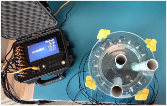
Figure 5. Measuring station with SmartEIT tomograph and physical model of the tank with electrodes and tubes immersed in water.

Several tens of measurements were made on such a physical model, adjusting the parameters of the mathematical model based on the generalized Laplace equation, which correctly generated measurement values based on a dense finite element mesh. Based on this model, a set of 50,000 cases containing both the measurements and the corresponding conductivity distributions was generated. In addition, Gaussian noise with standard deviation was added to each measurement value. Reference measurements were made several times with the tomograph. By analyzing the signals obtained from the electrodes, the noise was estimated, which averaged about 4% of the standard deviation of the reference measurements. Therefore, for reference, Gaussian white noise was added to the sonde generated from the electrodes in EIDORS, and then reconstructions were determined for the noisy signal using logistic regression models.

The basic properties of the reference model describe the field of view: number of electrodes: 16; type of electrodes: linear; number of nodes: 1338; number of finite elements: 2502. There are different types of wavelets. In this paper, we present the applications of the following wavelets: Daubechies ‘db1’, ‘db2’, ‘db7’; Coiflets, ‘coif1’, ‘coif2’; Symlets ‘sym1’, ‘sym2’); Biorthogonal ‘bior1.1’, ‘bior1.5’, ‘bior2.2’. Each finished element is a pixel of the tomographic image. The output image is, in fact, an illustration of the conductivity distribution of the individual mesh elements.

To assess the quality of the visual area reconstruction, below we present some basic Receiver Operating Characteristic (ROC) analyses [27]. For this purpose, the finite element that does not belong to the inclusions is described as a negative case (N) and interpreted as an element that belongs to the background. On the other hand, the finite element that belongs to the inclusions is taken as the positive case (P). Therefore, to determine the basic characteristics, the confusion matrix is first determined in the following way: TP (True Positive)—denotes the finite elements that correctly belong to the inclusion area; TN (True Negative)—the number of finite elements that are correctly recognized as belonging to the background; FP (False Positive)—the number of finite elements belonging to the background that are recognized as having belonged to the inclusion area (false alarm); FN (False Negative)—the number of finite elements belonging to the inclusion area but recognized as background.

We determine the basic coefficients as follows [27]:

$$\begin{array}{c}Accuracy=\frac{TP+TN}{TP+TN+FP+FN},\hfill \\ Sensivity=\frac{TP}{TP+FN},\hfill \\ Specificity=\frac{TN}{TN+FP},\hfill \\ PositivePredictiveValue=\frac{TP}{TP+FP},\hfill \\ NegativePredictiveValue=\frac{TN}{TN+FN},\hfill \\ DetectionRate=\frac{TP}{TP+TN+FP+FN}, \hfill \end{array}$$

To determine the ability of a classifier based on the use of logistic regression [15], we determine a curve describing the Receiver Operating Characteristic (ROC) curve [27]. The ROC curve shows the relationship between True Positive Rate (sensitivity on the Y-axis) and False Positive Rate (1-specificity on the X-axis) for different settings of cut-off levels (levels of class membership discrimination). Using logistic regression in EIT, the ROC curve shows the detection ability of a binary classifier that determines the affiliation of finite elements to the region of the inclusion for different settings of probability levels. The most optimal models can be determined by analyzing the class of models (a set of classifiers) using the ROC analysis (characterized by a higher TPR value for each established FPR). In some cases, when analyzing the ROC curves, determining the optimal classifier is quite difficult, while as the optimal classifier, we choose the one for which the Area under the Curve (AUC) is the greatest. This quantity is also included in Table 1, Table 2 and Table 3 describing the reconstructions.

Table 1. Summary of reconstruction of pattern presented in Figure 6.

	Elastic Net	db1	db2	db7	coif1	coif2	sym1	sym2	bior1.1	bior1.5	bior2.2
Accuracy	0.984	0.962	0.967	0.968	0.962	0.970	0.962	0.967	0.962	0.966	0.960
Sensitivity	0.830	0.528	0.651	0.368	0.472	0.462	0.528	0.651	0.528	0.481	0.453
Specificity	0.990	0.981	0.981	0.995	0.984	0.992	0.981	0.981	0.981	0.987	0.982
Pos Pred Value	0.793	0.549	0.605	0.750	0.568	0.731	0.549	0.605	0.549	0.622	0.527
Neg Pred Value	0.992	0.979	0.985	0.973	0.977	0.977	0.979	0.985	0.979	0.977	0.976
Detection Rate	0.035	0.022	0.028	0.016	0.020	0.020	0.022	0.028	0.022	0.020	0.019
AUC	0.990	0.827	0.905	0.757	0.777	0.781	0.827	0.905	0.827	0.796	0.780
$\kappa$	0.802	0.518	0.610	0.479	0.496	0.552	0.518	0.610	0.518	0.525	0.466
${\chi }^2$	0.390	0.094	0.598	35.112	3.074	19.253	0.094	0.598	0.094	6.151	1.941
p-value	0.532	0.759	0.440	0.000	0.080	0.000	0.759	0.440	0.759	0.013	0.164

Table 2. Summary of reconstruction of pattern presented in Figure 8.

	Elastic Net	db1	db2	db7	coif1	coif2	sym1	sym2	bior1.1	bior1.5	bior2.2
Accuracy	0.992	0.994	0.993	0.979	0.994	0.982	0.994	0.993	0.994	0.993	0.990
Sensitivity	0.940	0.867	0.855	0.386	0.904	0.470	0.867	0.855	0.867	0.819	0.843
Specificity	0.994	0.999	0.998	1.000	0.997	0.999	0.999	0.998	0.999	0.999	0.995
Pos Pred Value	0.839	0.960	0.922	0.970	0.915	0.951	0.960	0.922	0.960	0.958	0.864
Neg Pred Value	0.998	0.995	0.995	0.979	0.997	0.982	0.995	0.995	0.995	0.994	0.995
Detection Rate	0.031	0.029	0.028	0.013	0.030	0.016	0.029	0.028	0.029	0.027	0.028
AUC	0.999	1.000	0.999	0.991	0.999	0.992	1.000	0.999	1.000	0.999	0.999
$\kappa$	0.882	0.909	0.884	0.543	0.906	0.621	0.909	0.884	0.909	0.879	0.849
${\chi }^2$	4.050	3.500	1.389	46.173	0.000	36.543	3.500	1.389	3.500	6.722	0.042
p-value	0.044	0.061	0.239	0.000	1.000	0.000	0.061	0.239	0.061	0.010	0.838

Table 3. Summary of reconstruction of pattern presented in Figure 10.

	Elastic Net	db1	db2	db7	coif1	coif2	sym1	sym2	bior1.1	bior1.5	bior2.2
Accuracy	0.961	0.940	0.931	0.926	0.939	0.904	0.940	0.931	0.940	0.937	0.941
Sensitivity	0.662	0.505	0.354	0.192	0.444	0.212	0.505	0.354	0.505	0.495	0.465
Specificity	0.987	0.977	0.981	0.989	0.982	0.964	0.977	0.981	0.977	0.975	0.982
Pos Pred Value	0.814	0.654	0.614	0.594	0.677	0.336	0.654	0.614	0.654	0.632	0.692
Neg Pred Value	0.971	0.958	0.946	0.934	0.954	0.934	0.958	0.946	0.958	0.957	0.955
Detection Rate	0.052	0.040	0.028	0.015	0.035	0.017	0.040	0.028	0.040	0.039	0.037
AUC	0.987	0.932	0.913	0.854	0.936	0.755	0.932	0.913	0.932	0.936	0.938
$\kappa$	0.786	0.566	0.424	0.333	0.486	0.207	0.566	0.424	0.566	0.532	0.474
${\chi }^2$	0.203	0.025	0.043	23.338	17.128	1.308	0.025	0.043	0.025	0.729	4.380
p-value	0.653	0.873	0.835	0.000	0.000	0.253	0.873	0.835	0.873	0.393	0.036

To assess the reliability of reconstruction (agreement between pattern and reconstruction), we estimate Cohen’s kappa ratio as follows:

$$\kappa =\frac{2\left(TP·TN-FN·FP\right)}{\left(TP+FP\right)\left(FP+TN\right)+\left(TP+FN\right)\left(FN+TN\right)}.$$

Generally, $\kappa \in \left[0,1\right]$. When kappa has the higher value, the agreement between pattern and reconstruction is higher, and when there is complete agreement $\kappa =1$.

To verify whether there is a significant disagreement between pattern and reconstruction, we apply McNemar’s test. This test compares the sensitivity and specificity of reconstruction. The McNemar’s test statistic is defined as follows:

$${\chi }^2=\frac{{\left(FP-FN\right)}^2}{FN+FP}$$

and has ${\chi }^2$ distribution with 1 degree of freedom.

Three patterns are shown below with their reconstructions. The patterns were simulated in MATLAB, and signals were determined as voltage vectors from the electrodes using EIDORS. Figure 6, Figure 7, Figure 8, Figure 9, Figure 10 and Figure 11 summary the image reconstruction for the example 1. Figure 6, Figure 8 and Figure 10 show the results of these reconstructions, but Figure 7, Figure 9 and Figure 11 show the ROC curve for reconstructions presented in Figure 6, Figure 8 and Figure 10. Table 1, Table 2 and Table 3 present the basic coefficient of ROC analysis, Cohen’s kappa, McNemar’s test statistic and p-value.

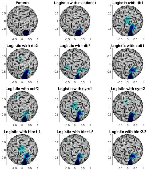
Figure 6. Image reconstruction for one object—example 1.

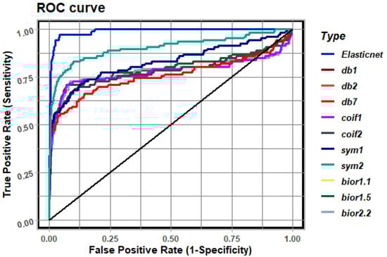
Figure 7. ROC analysis for example 1.

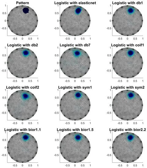
Figure 8. Image reconstruction for one object—example 2.

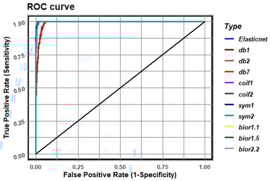
Figure 9. ROC analysis for example 2.

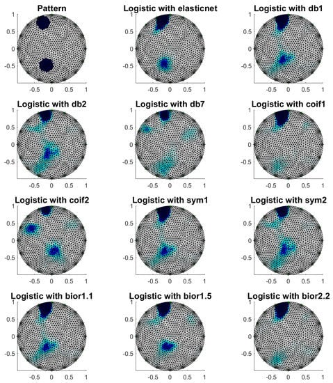
Figure 10. Image reconstruction for two objects—example 3.

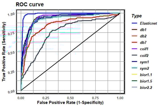
Figure 11. ROC analysis for example 3.

In order to verify the performed numerical tests, measurements were made on a laboratory tank. The image reconstruction results based on logistic regression with elastic net and different wavelets decompositions are shown in Figure 12, Figure 13, Figure 14, Figure 15, Figure 16, Figure 17, Figure 18, Figure 19 and Figure 20.

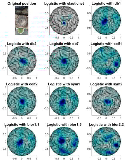
Figure 12. Image reconstruction with the centrally placed phantom.

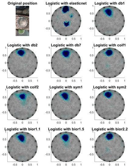
Figure 13. Image reconstruction with a phantom at electrode 1.

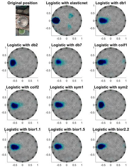
Figure 14. Image reconstruction with a phantom at electrode 13.

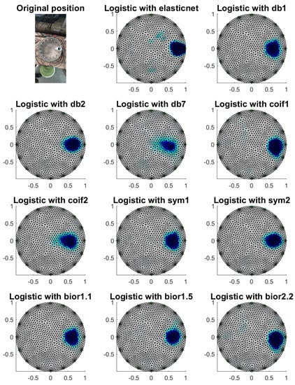
Figure 15. Image reconstruction with a phantom at electrode 5.

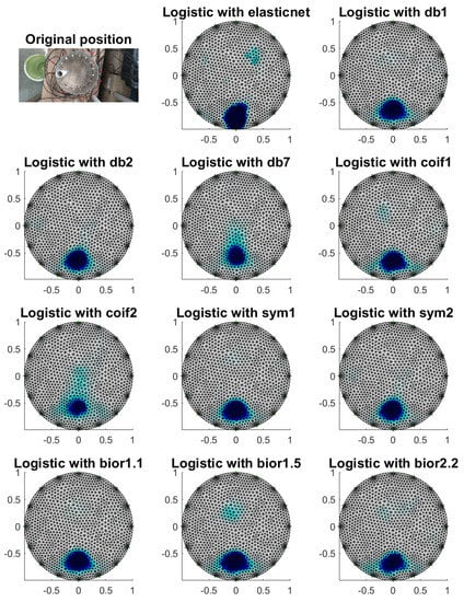
Figure 16. Image reconstruction with a phantom at electrode 9.

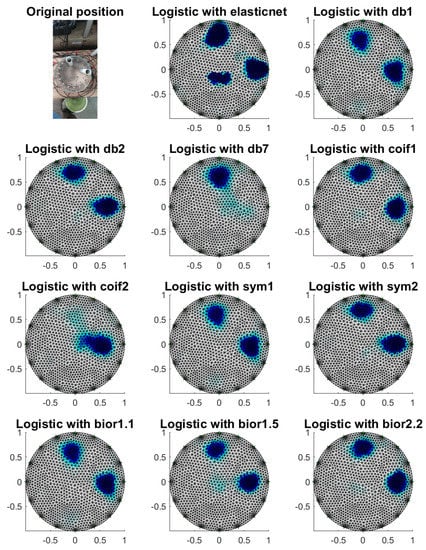
Figure 17. Image reconstruction with phantoms at electrodes 1 and 5.

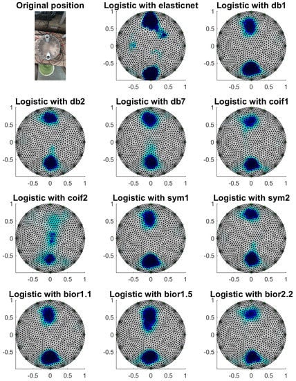
Figure 18. Image reconstruction with phantoms at electrodes 1 and 9.

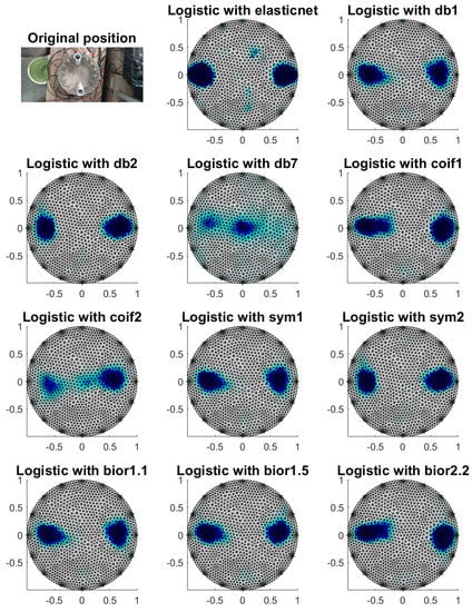
Figure 19. Image reconstruction with phantoms at electrodes 5 and 13.

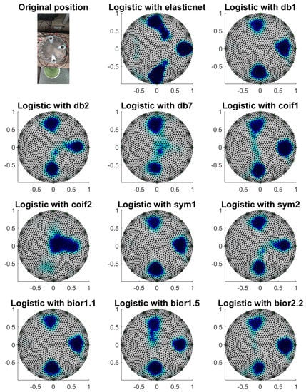
Figure 20. Image reconstruction with phantoms at electrodes 1, 5 and 9.

4. Discussion

The monitoring system presented is designed to automate, analyze and optimize processes using industrial tomography to analyze without disturbing its interior. This solution allows for better monitoring and control of processes. The system was designed using electrical tomography, which is used to study technological processes. An image reconstruction algorithm then processes the collected data. The main challenge in electrical tomography is the construction of precise measurement devices and image reconstruction methods. The idea of the measurement system was based on tomographic sensors for data collection and gathering and through appropriate communication protocols for processing in the computing cloud.

One of the problems in EIT image reconstruction using binary classifiers is the selection of variables that significantly influence the classifier’s result. In this study, the elastic net technique and wavelet decomposition were used to reduce the dimensions of the signal obtained from the electrodes. To answer the question of which method gives the best reconstruction, the same patterns were simulated at the beginning. Next, the reconstructed images have been compared with the patterns. Since visual assessment is not objective enough, popular quantitative Receiver Operating Characteristics were estimated: Accuracy, Sensitivity, Specificity, Positive Predictive Value, Negative Predictive Value, Detection Rate and AUC. Additionally, the assessments described the reliability of reconstructions (Cohen’s kappa) and the tests of disagreement between pattern and reconstruction (McNemar’s test) were provided.

Analyzing such characteristics as accuracy (the proportion of the visual area that the model correctly recognized) and specificity (the proportion of correctly recognized finite elements belonging to the background) is quite accurate. Thus, the quality of reconstruction is quite good. Nevertheless, from sensitivity (the proportion of correctly recognized finite elements belonging to the inclusion) analysis, we see that the best reconstructions were obtained by applying “db1”, “db2”, “sym1”, “sym2” and “bior1.1” wavelet decompositions. An identical result is obtained by analyzing the values of Cohen’s kappa. Quite good reliability of reconstructions was obtained for “db1”, “db2”, “sym1”, “sym2” and “bior1.1” wavelet decompositions too. By analyzing the AUC values, the best reconstructions are obtained for the dimension reduction techniques: elastic net and signal decomposition using “db1”, “db2”, “coif1”, “sym1” and “bior1.1”.

Based on McNemar’s test, we can conclude that for examples 1–2 at a significance level of 0.05, the null hypothesis (pattern and reconstruction are consistent or disagreement is irrelevant) is rejected in favor of the alternative hypothesis (disagreement between pattern and reconstruction is significant) for “db7”, “coif2” and “bior1.5” wavelet decompositions, and “db7” and “coif1” wavelet decompositions for example 3.

When reconstructing for real data, visually satisfactory results were obtained for signal decomposition using wavelets “db1”, “db2”, “coif1”, “sym1”, “sym2”, “bior1.1” and “bior1.5”. Quite poor reconstructions for cases where more than one object in the visual area were obtained for decomposition using “coif2”.

5. Conclusions

This study aimed to develop algorithms based on Logistic Regression and Wavelet Preprocessing methods to solve the inverse problem in EIT. The research focused on the development and comparison of algorithms and models for image reconstruction. All the algorithms presented are well suited to practical implementations in EIT. Depending on the number of measuring sensors used and the analyzed patterns, the obtained quality of the reconstructed images varies in different methods. To perform the reconstruction in EIT, we estimate the conductance for each finite element typically. In the presented case, we calculate the probability that a finite element belongs to an inclusion. For this purpose, we create a logistic regression model for each finite element. In this way, a logistic regression-based reconstruction is defined as a set of logistic regression models resting on the finite elements.

The use of logistic regression for image reconstruction in EIT should be preceded by selecting independent variables for each finite element separately. In order to reduce the dimensions of the independent variables, the elastic net technique was used in this work, as well as wavelet decomposition of signals, which is a good alternative tool to the elastic net. However, in the case of several objects in the field of view, objects located in the center are recognized poorly.

Further work could focus on ROC analysis for finite elements located in the center of the field of view, determining the thresholding for binary classifiers for finite elements depending on the position of the element in the field of view, and improving reconstruction in the center of the field of view (improving classifiers for finite elements further away from the electrodes). For further research and analysis, the decompositions “db1”, “db2”, “coif1”, “sym1”, “sym2” and “bior1.1” will be used to reduce the over dimensionality of independent variables in logistic regression models. Additionally, we investigated the dependence of the fit quality of logistic models (e.g., using the Hosmer–Lemeshow test) at different locations in the field of view. It could be the subject of a larger study to improve the quality of the reconstruction further.

Thus, the presented research results contain essential information that may accelerate the development of machine learning methods in industrial tomography. Furthermore, the research contributes to improving the efficiency of tomographic imaging with the use of electrical properties.

References

- Wajman, R.; Banasiak, R.; Babout, L. On the Use of a Rotatable ECT Sensor to Investigate Dense Phase Flow: A Feasibility Study. Sensors 2020, 20, 4854. [Google Scholar] [CrossRef] [PubMed]
- Rybak, G.; Strzecha, K. Short-Time Fourier Transform Based on Metaprogramming and the Stockham Optimization Method. Sensors 2021, 21, 4123. [Google Scholar] [CrossRef]
- Rymarczyk, T.; Kłosowski, G.; Hoła, A.; Sikora, J.; Wołowiec, T.; Tchórzewski, P.; Skowron, S. Comparison of Machine Learning Methods in Electrical Tomography for Detecting Moisture in Building Walls. Energies 2021, 14, 2777. [Google Scholar] [CrossRef]
- Rymarczyk, T.; Nita, P.; Vejar, A.; Woś, M.; Stefaniak, B.; Adamkiewicz, P. Wearable mobile measuring device based on electrical tomography. Prz. Elektrotech. 2019, 95, 211–214. [Google Scholar]
- Romanowski, A.; Chaniecki, Z.; Koralczyk, A.; Wozniak, M.; Nowak, A.; Kucharski, P.; Jaworski, T.; Malaya, M.; Rozga, P.; Grudzien, K. Interactive Timeline Approach for Contextual Spatio-Temporal ECT Data Investigation. Sensors 2020, 20, 4793. [Google Scholar] [CrossRef] [PubMed]
- Mosorov, V.; Rybak, G.; Sankowski, D. Plug Regime Flow Velocity Measurement Problem Based on Correlability Notion and Twin Plane Electrical Capacitance Tomography: Use Case. Sensors 2021, 21, 2189. [Google Scholar] [CrossRef] [PubMed]
- Voss, A.; Pour-Ghaz, M.; Vauhkonen, M.; Seppanen, A. Retrieval of the saturated hydraulic conductivity of cement-based materials using electrical capacitance tomography. Cem. Concr. Compos. 2020, 112, 103639. [Google Scholar] [CrossRef]
- Shi, X.W.; Tan, C.; Dong, F.; dos Santos, E.N.; da Silva, M.J. Conductance Sensors for Multiphase Flow Measurement: A Review. IEEE Sens. J. 2021, 21, 12913–12925. [Google Scholar] [CrossRef]
- Midura, M.; Wróblewski, P.; Wanta, D.; Domański, G.; Stosio, M.; Kryszyn, J.; Smolik, W.T. The system for complex magnetic susceptibility measurement of nanoparticles with 3d printed carcass for integrated receive coils. Inform. Autom. Pomiary W Gospod. I Ochr. Śr. 2021, 11, 4–9. [Google Scholar] [CrossRef]
- Rymarczyk, T.; Kłosowski, G.; Tchórzewski, P.; Cieplak, T.; Kozłowski, E. Area monitoring using the ERT method with multisensor electrodes. Prz. Elektrotech. 2019, 95, 153–156. [Google Scholar] [CrossRef] [Green Version]
- Chen, B.; Abascal, J.; Soleimani, M. Extended Joint Sparsity Reconstruction for Spatial and Temporal ERT Imaging. Sensors 2018, 18, 4014. [Google Scholar] [CrossRef] [PubMed] [Green Version]
- Ratheesh, K.M.; Seah, L.K.; Murukeshan, V.M. Spectral phase-based automatic calibration scheme for swept source-based optical coherence tomography systems. Phys. Med. Biol. 2016, 61, 7652. [Google Scholar] [CrossRef]
- Koulountzios, P.; Aghajanian, S.; Rymarczyk, T.; Koiranen, T.; Soleimani, M. An Ultrasound Tomography Method for Monitoring CO2 Capture Process Involving Stirring and CaCO3 Precipitation. Sensors 2021, 21, 6995. [Google Scholar] [CrossRef] [PubMed]
- Koulountzios, P.; Rymarczyk, T.; Soleimani, M. A triple-modality ultrasound computed tomography based on full-waveform data for industrial processes. IEEE Sens. J. 2021, 21, 20896–20909. [Google Scholar] [CrossRef]
- Dusek, J.; Mikulka, J. Measurement-Based Domain Parameter Optimisation in Electrical Impedance Tomography Imaging. Sensors 2021, 21, 2507. [Google Scholar] [CrossRef] [PubMed]
- Rymarczyk, T.; Kozłowski, E.; Kłosowski, G. Electrical impedance tomography in 3D flood embankments testing—Elastic net approach. Trans. Inst. Meas. Control. 2020, 42, 680–690. [Google Scholar] [CrossRef]
- Dušek, J.; Hladký, D.; Mikulka, J. Electrical Impedance Tomography Methods and Algorithms Processed with a GPU. In Proceedings of the 2017 Progress in Electromagnetics Research Symposium—Spring (PIERS), St. Petersburg, Russia, 22–25 May 2017; pp. 1710–1714. [Google Scholar]
- Liu, S.H.; Huang, Y.M.; Wu, H.C.; Tan, C.; Jia, J.B. Efficient Multitask Structure-Aware Sparse Bayesian Learning for Frequency-Difference Electrical Impedance Tomography. IEEE Trans. Ind. Inform. 2021, 17, 463–472. [Google Scholar] [CrossRef] [Green Version]
- Adler, A.; Lionheart, W.R. Uses and abuses of EIDORS: An extensible software base for EIT. Physiol. Meas. 2006, 27, 25–42. [Google Scholar] [CrossRef] [Green Version]
- Kozłowski, E.; Mazurkiewicz, D.; Żabiński, T.; Prucnal, S.; Sęp, J. Assessment model of cutting tool condition for real-time supervision system. Eksploat. I Niezawodn. 2019, 21, 679–685. [Google Scholar] [CrossRef]
- Sekulska-Nalewajko, J.; Gocławski, J.; Korzeniewska, E. A method for the assessment of textile pilling tendency using optical coherence tomography. Sensors 2020, 20, 3687. [Google Scholar] [CrossRef] [PubMed]
- Szczesny, A.; Korzeniewska, E. Selection of the method for the earthing resistance measurement. Prz. Elektrotech. 2018, 94, 178–181. [Google Scholar]
- Daniewski, K.; Kosicka, E.; Mazurkiewicz, D. Analysis of the correctness of determination of the effectiveness of maintenance service actions. Manag. Prod. Eng. Rev. 2018, 9, 20–25. [Google Scholar]
- Kłosowski, G.; Rymarczyk, T.; Wójcik, D.; Skowron, S.; Adamkiewicz, P. The Use of Time-Frequency Moments as Inputs of LSTM Network for ECG Signal Classification. Electronics 2020, 9, 1452. [Google Scholar] [CrossRef]
- Fiala, P.; Bartušek, K.; Dědková, J.; Dohnal, P. EMG field analysis in dynamic microscopic/nanoscopic models of matter. Inform. Autom. Pomiary W Gospod. I Ochr. Sr. 2019, 9, 4–10. [Google Scholar] [CrossRef]
- Rzasa, M.R.; Czapla-Nielacna, B. Analysis of the Influence of the Vortex Shedder Shape on the Metrological Properties of the Vortex Flow Meter. Sensors 2021, 21, 4697. [Google Scholar] [CrossRef]
- Fawcett, T. An Introduction to ROC Analysis. Pattern Recognit. Lett. 2006, 27, 861–874. [Google Scholar] [CrossRef]
- Yan, X.; Su, X.G. Linear Regression Analysis; World Scientific Publishing Co.: Singapore, 2009. [Google Scholar]
- Kuhn, M.; Johnson, K. Applied Predictive Modelling; Springer: Berlin/Heidelberg, Germany, 2016. [Google Scholar]
- Schonlau, M.; Zou, R.Y. The random forest algorithm for statistical learning. Stata J. 2020, 20, 3–29. [Google Scholar] [CrossRef]
- Ayyadevara, V.K. Gradient Boosting Machine. In Pro Machine Learning Algorithms; Apress: Berkeley, CA, USA, 2018. [Google Scholar]
- Urbanski, P. Principal component and partial least squares regressions in the calibration of nucleonic gauges. Appl. Radiat. Isot. 1994, 45, 659–667. [Google Scholar] [CrossRef]
- Liu, S.; Wu, H.; Huang, Y.; Yang, Y.; Jia, J. Accelerated Structure-Aware Sparse Bayesian Learning for 3D Electrical Impedance Tomography. IEEE Trans. Ind. Inform. 2019, 15, 5033–5041. [Google Scholar] [CrossRef]
- Walnut, D.F. An Introduction to Wavelet Analysis; Springer Science & Business Media: Berlin/Heidelberg, Germany, 2002. [Google Scholar]
- Daubechies, I. Orthonormal Bases of Compactly Supported Wavelets. Commun. Pure Appl. Math. 1992, 41, 909–996. [Google Scholar] [CrossRef] [Green Version]
- Percival, D.B.; Walden, A. Wavelet Methods for Time Series Analysis; Cambridge University Press: Cambridge, UK, 2000; Volume 4. [Google Scholar]
Publisher’s Note: MDPI stays neutral with regard to jurisdictional claims in published maps and institutional affiliations. |
© 2021 by the authors. Licensee MDPI, Basel, Switzerland. This article is an open access article distributed under the terms and conditions of the Creative Commons Attribution (CC BY) license (https://creativecommons.org/licenses/by/4.0/).