
Forecasting Brazilian Ethanol Spot Prices Using LSTM

 , , and
Abstract
1. Introduction
2. Related Work
3. Methodology
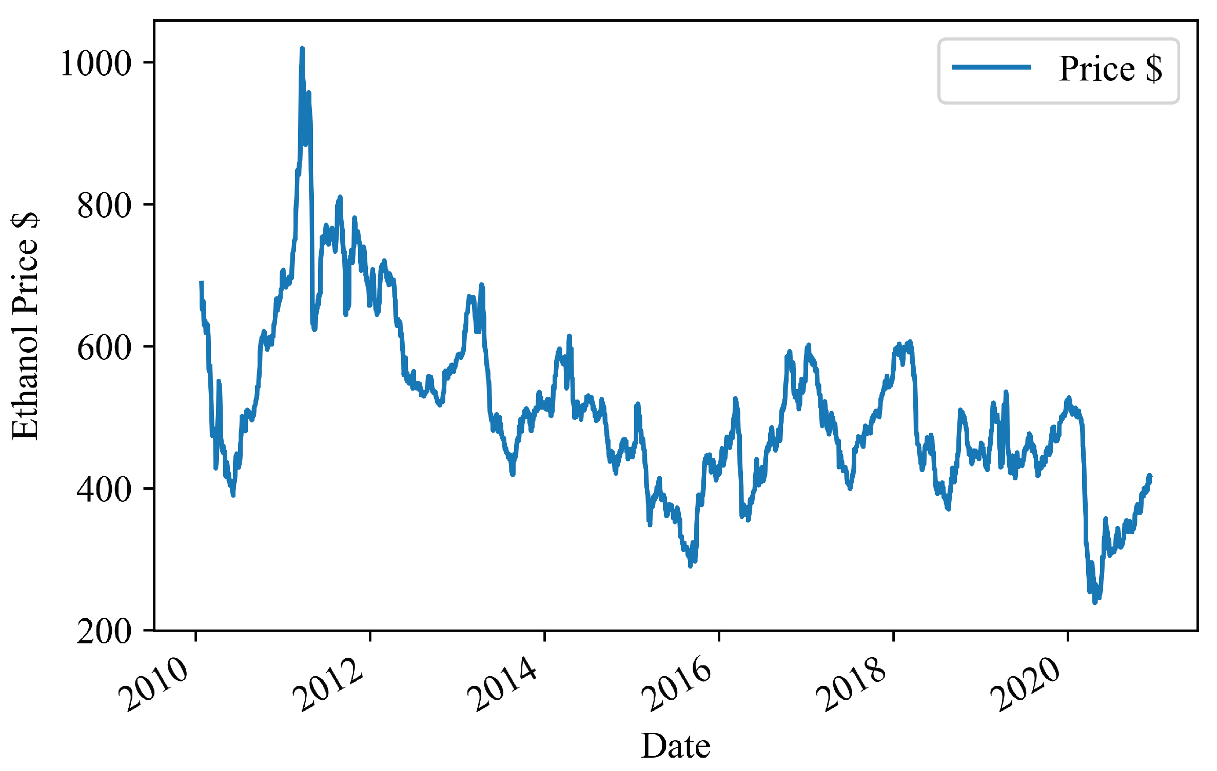
3.1. Data
Data Pre-Processing
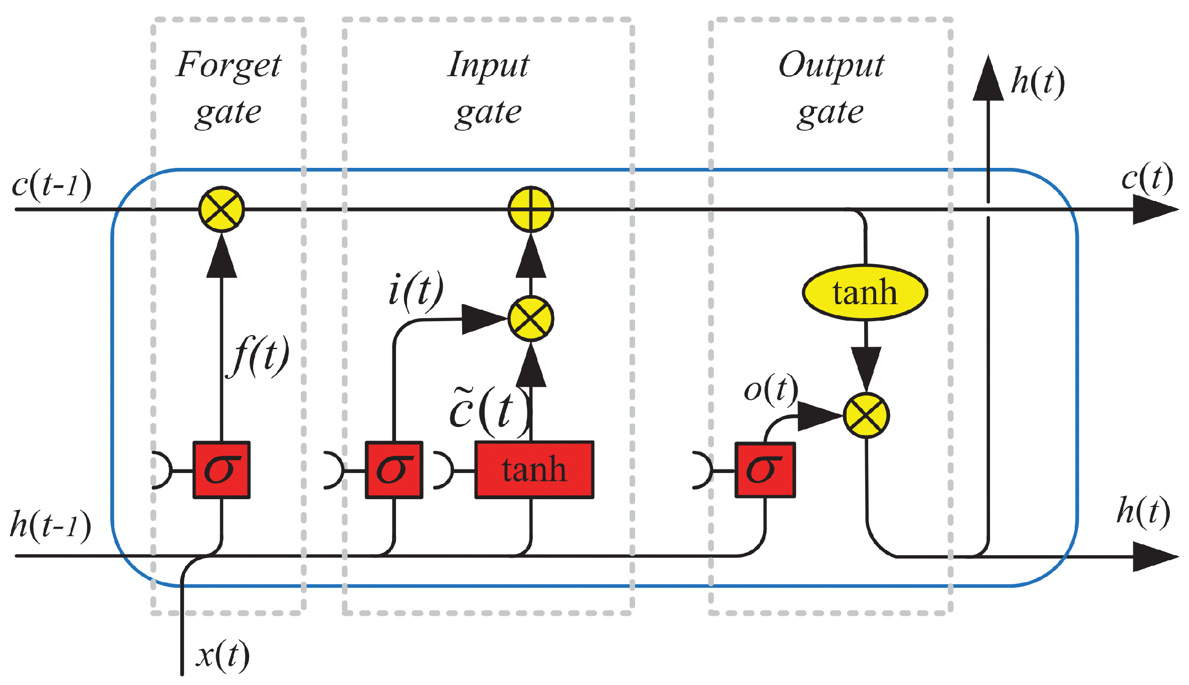
3.2. LSTM Networks
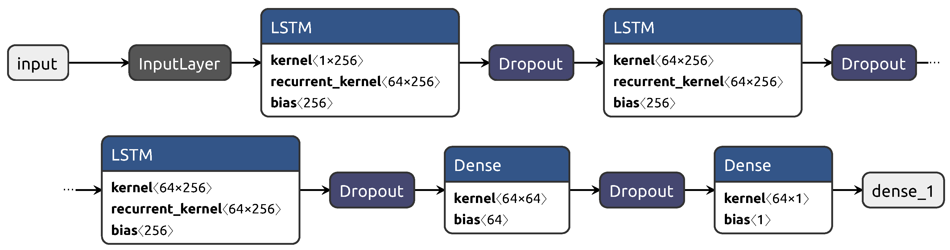
3.3. Proposed Model and Benchmarks
4. Results and Discussions
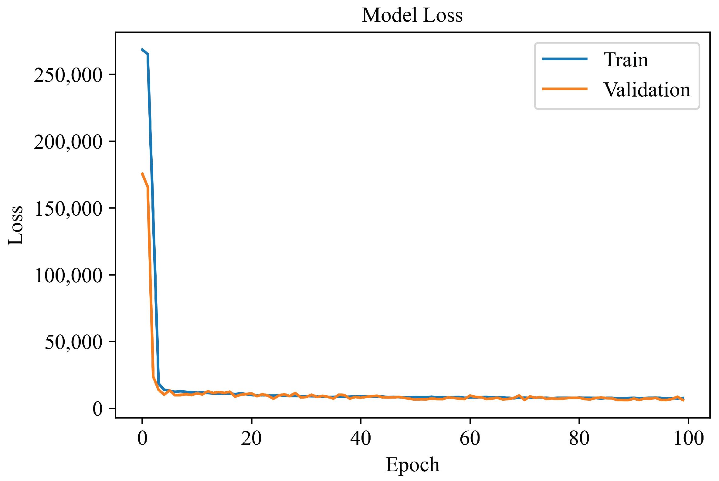
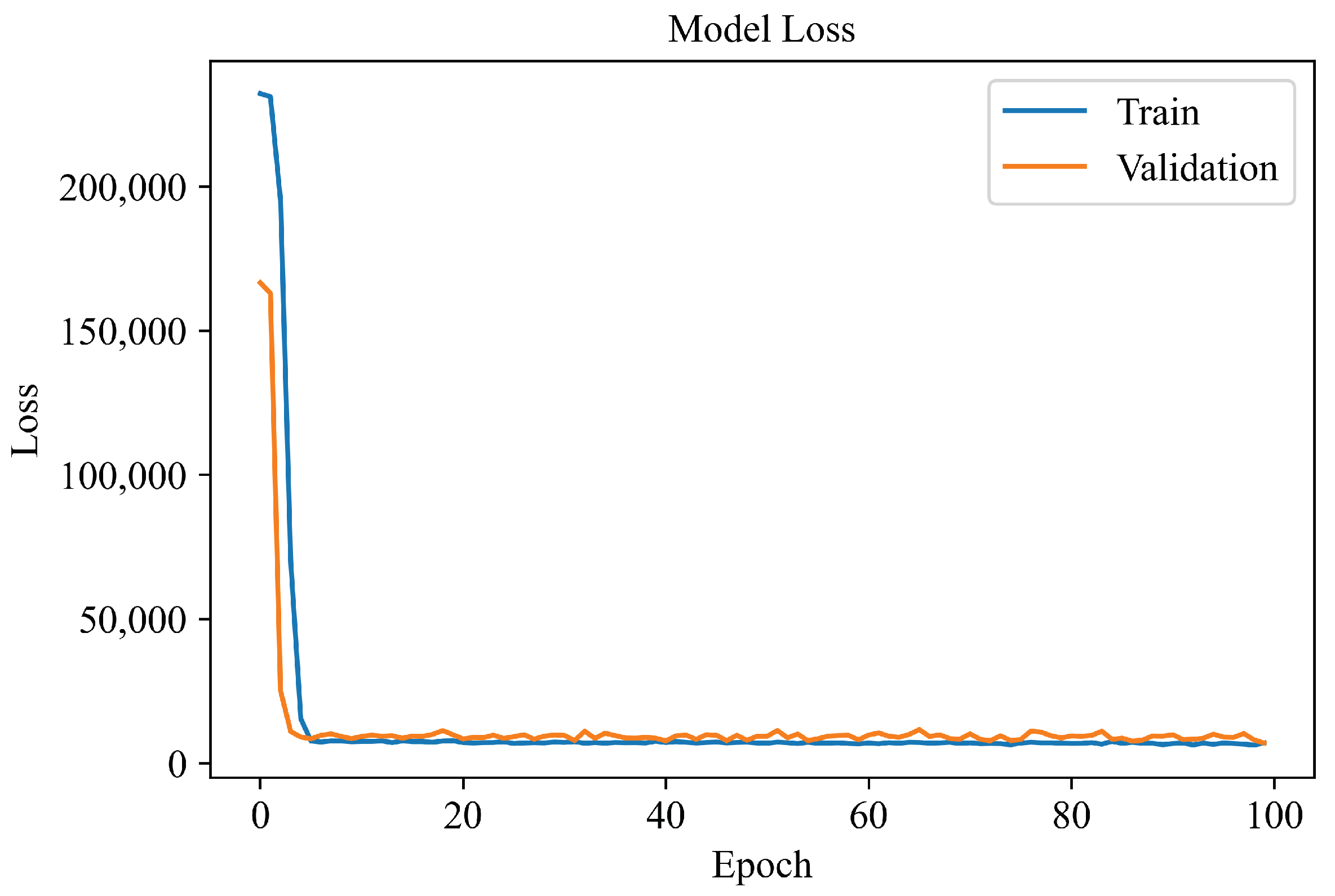
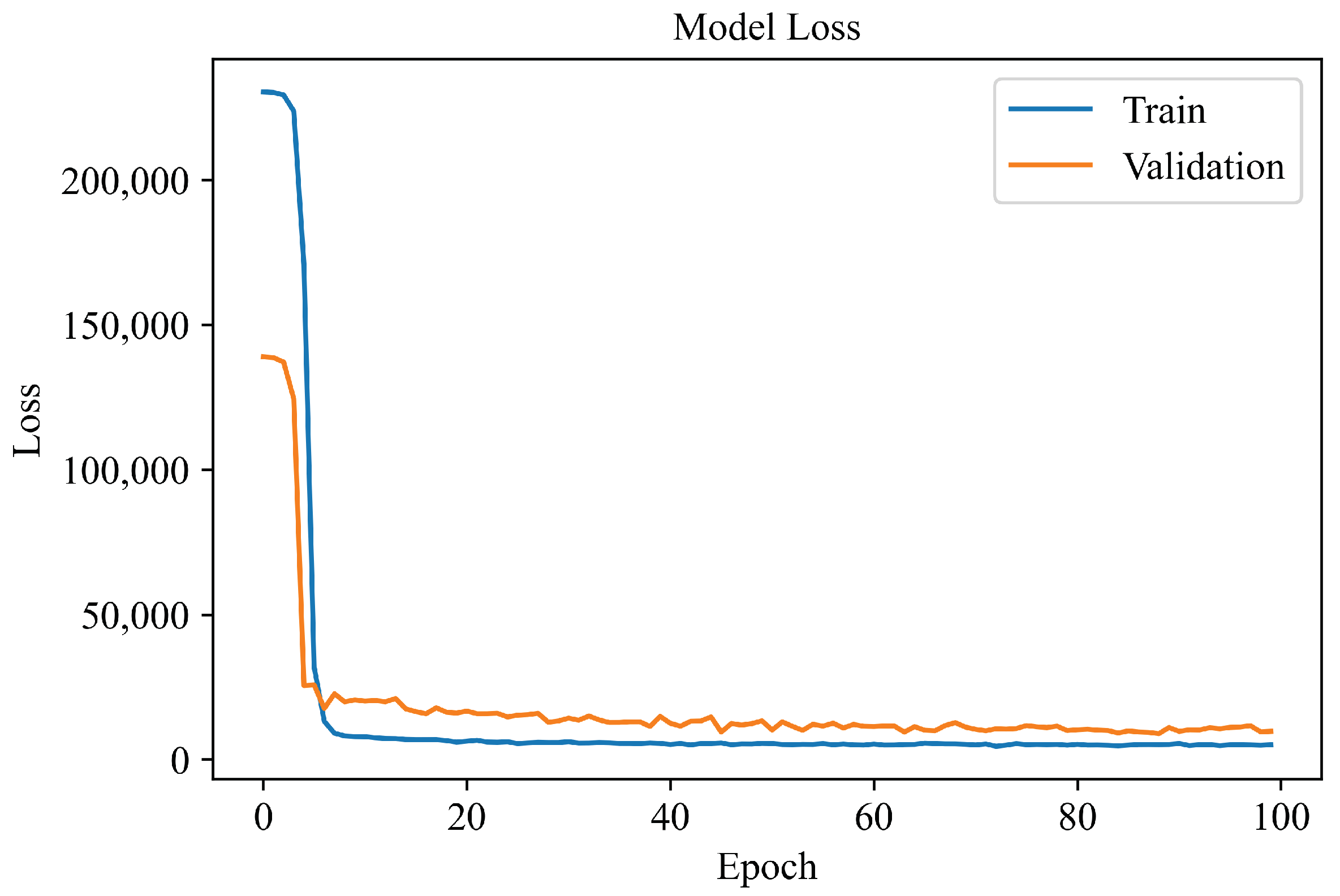
4.1. Learning Curves
4.2. Forecasting Results
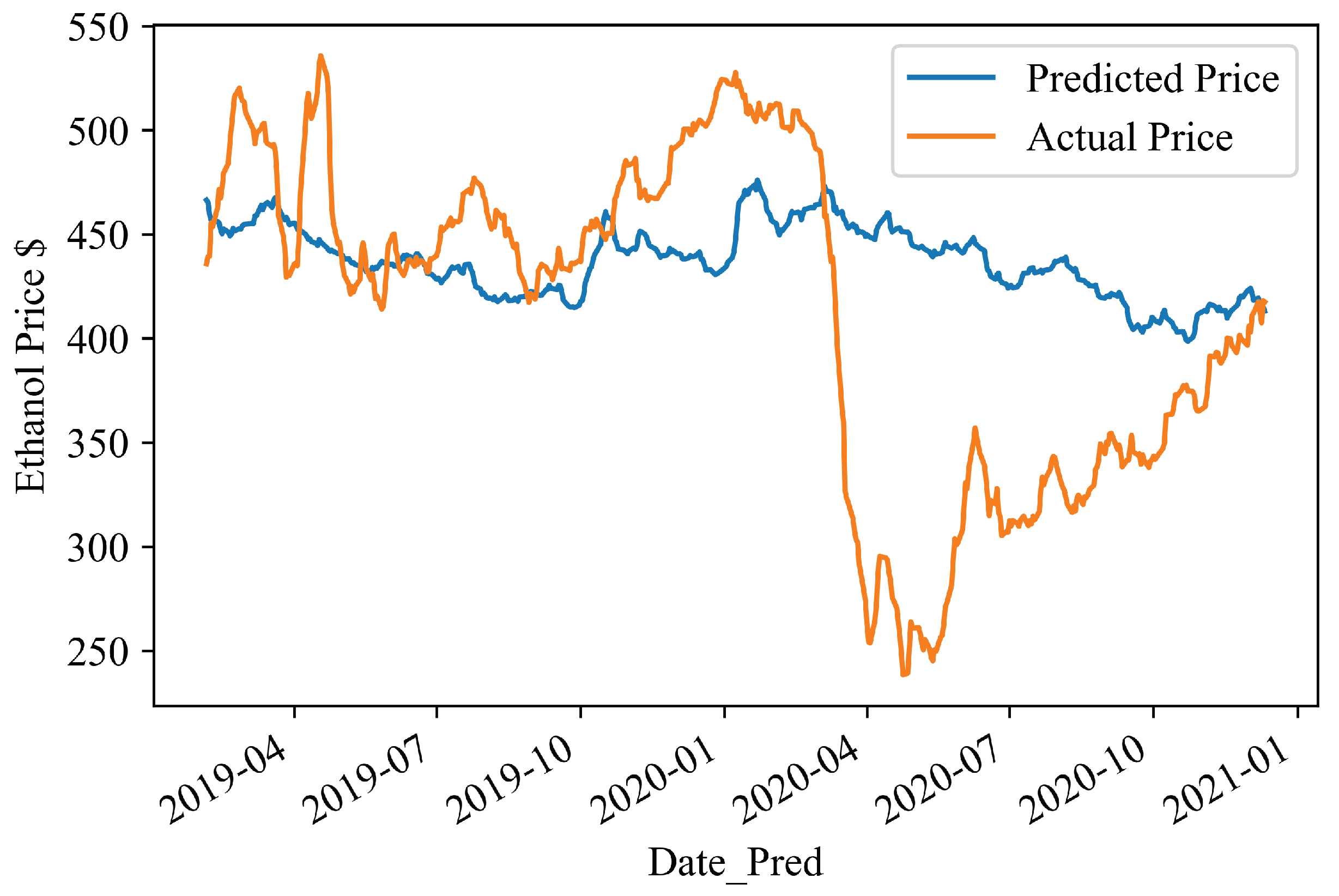
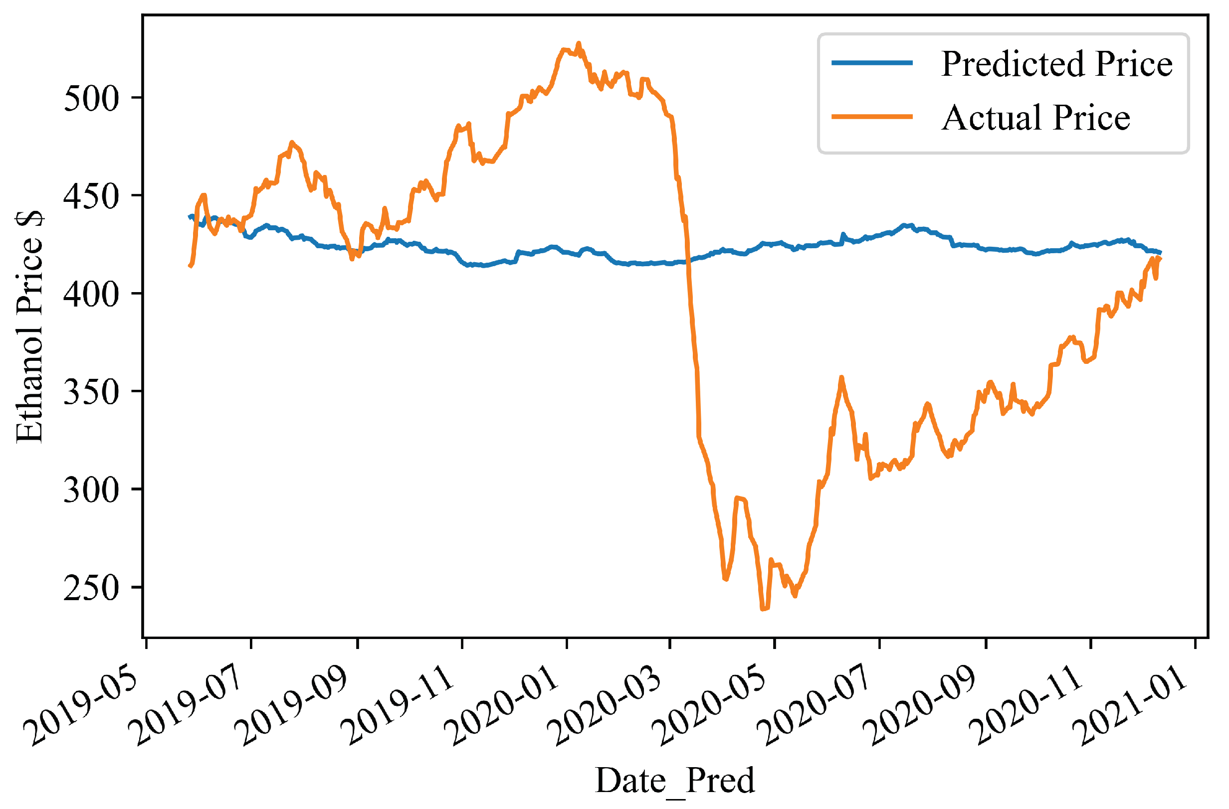
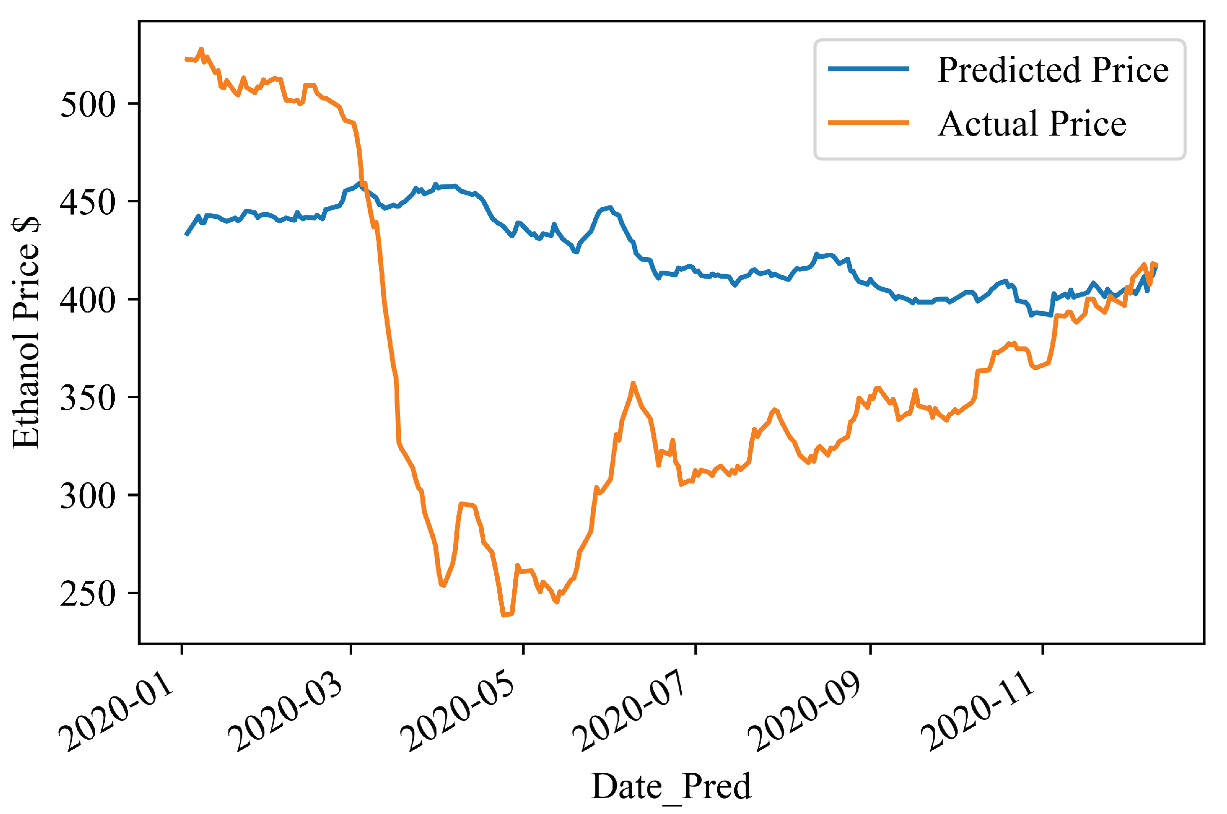
4.3. Visualising the Predictions
5. Conclusions
Author Contributions
Funding
Institutional Review Board Statement
Informed Consent Statement
Data Availability Statement
Conflicts of Interest
References
- Goldemberg, J. The ethanol program in Brazil. Environ. Res. Lett. 2006, 1, 014008. [Google Scholar] [CrossRef]
- Silva, G.P.D.; Araújo, E.F.D.; Silva, D.O.; Guimarães, W.V. Ethanolic fermentation of sucrose, sugarcane juice and molasses by Escherichia coli strain KO11 and Klebsiella oxytoca strain P2. Braz. J. Microbiol. 2005, 36, 395–404. [Google Scholar] [CrossRef]
- Lopes, M.L.; de Lima Paulillo, S.C.; Godoy, A.; Cherubin, R.A.; Lorenzi, M.S.; Giometti, F.H.C.; Bernardino, C.D.; de Amorim Neto, H.B.; de Amorim, H.V. Ethanol production in Brazil: A bridge between science and industry. Braz. J. Microbiol. 2016, 47, 64–76. [Google Scholar] [CrossRef] [PubMed]
- Ministry of Agriculture, Fisheries and Supply—Ethanol Archives. Available online: https://www.gov.br/agricultura/pt-br/assuntos/sustentabilidade/agroenergia/arquivos-etanol-comercio-exterior-brasileiro/ (accessed on 11 November 2021).
- Carpio, L.G.T. The effects of oil price volatility on ethanol, gasoline, and sugar price forecasts. Energy 2019, 181, 1012–1022. [Google Scholar] [CrossRef]
- EIA—Today in Energy. Available online: https://www.eia.gov/todayinenergy/detail.php?id=47956 (accessed on 11 October 2021).
- Hira, A.; de Oliveira, L.G. No substitute for oil? How Brazil developed its ethanol industry. Energy Policy 2009, 37, 2450–2456. [Google Scholar] [CrossRef]
- David, S.A.; Inácio, C.; Tenreiro Machado, J.A. Quantifying the predictability and efficiency of the cointegrated ethanol and agricultural commodities price series. Appl. Sci. 2019, 9, 5303. [Google Scholar] [CrossRef]
- David, S.; Quintino, D.; Inacio, C.; Machado, J. Fractional dynamic behavior in ethanol prices series. J. Comput. Appl. Math. 2018, 339, 85–93. [Google Scholar] [CrossRef]
- Tapia Carpio, L.G.; Simone de Souza, F. Competition between second-generation ethanol and bioelectricity using the residual biomass of sugarcane: Effects of uncertainty on the production mix. Molecules 2019, 24, 369. [Google Scholar] [CrossRef] [PubMed]
- Herrera, G.P.; Constantino, M.; Tabak, B.M.; Pistori, H.; Su, J.J.; Naranpanawa, A. Long-term forecast of energy commodities price using machine learning. Energy 2019, 179, 214–221. [Google Scholar] [CrossRef]
- de Araujo, F.H.A.; Bejan, L.; Rosso, O.A.; Stosic, T. Permutation entropy and statistical complexity analysis of Brazilian agricultural commodities. Entropy 2019, 21, 1220. [Google Scholar] [CrossRef]
- Barboza, F.; Kimura, H.; Altman, E. Machine learning models and bankruptcy prediction. Expert Syst. Appl. 2017, 83, 405–417. [Google Scholar] [CrossRef]
- Alameer, Z.; Fathalla, A.; Li, K.; Ye, H.; Jianhua, Z. Multistep-ahead forecasting of coal prices using a hybrid deep learning model. Resour. Policy 2020, 65, 101588. [Google Scholar] [CrossRef]
- Sun, W.; Zhang, J. Carbon Price Prediction Based on Ensemble Empirical Mode Decomposition and Extreme Learning Machine Optimized by Improved Bat Algorithm Considering Energy Price Factors. Energies 2020, 13, 3471. [Google Scholar] [CrossRef]
- Bouri, E.; Dutta, A.; Saeed, T. Forecasting ethanol price volatility under structural breaks. Biofuels Bioprod. Biorefining 2021, 15, 250–256. [Google Scholar] [CrossRef]
- Pokrivčák, J.; Rajčaniová, M. Crude oil price variability and its impact on ethanol prices. Agric. Econ. 2011, 57, 394–403. [Google Scholar] [CrossRef]
- Bastianin, A.; Galeotti, M.; Manera, M. Ethanol and field crops: Is there a price connection? Food Policy 2016, 63, 53–61. [Google Scholar] [CrossRef]
- Bildirici, M.; Guler Bayazit, N.; Ucan, Y. Analyzing Crude Oil Prices under the Impact of COVID-19 by Using LSTARGARCHLSTM. Energies 2020, 13, 2980. [Google Scholar] [CrossRef]
- Ding, S.; Zhang, Y. Cross market predictions for commodity prices. Econ. Model. 2020, 91, 455–462. [Google Scholar] [CrossRef]
- Kulkarni, S.; Haidar, I. Forecasting model for crude oil price using artificial neural networks and commodity futures prices. arXiv 2009, arXiv:0906.4838. [Google Scholar]
- Liu, Y.; Yang, C.; Huang, K.; Gui, W. Non-ferrous metals price forecasting based on variational mode decomposition and LSTM network. Knowl.-Based Syst. 2020, 188, 105006. [Google Scholar] [CrossRef]
- Hu, Y.; Ni, J.; Wen, L. A hybrid deep learning approach by integrating LSTM-ANN networks with GARCH model for copper price volatility prediction. Phys. A Stat. Mech. Its Appl. 2020, 557, 124907. [Google Scholar] [CrossRef]
- Zhou, B.; Zhao, S.; Chen, L.; Li, S.; Wu, Z.; Pan, G. Forecasting Price Trend of Bulk Commodities Leveraging Cross-Domain Open Data Fusion. ACM Trans. Intell. Syst. Technol. 2020, 11, 1–26. [Google Scholar] [CrossRef]
- Ouyang, H.; Wei, X.; Wu, Q. Agricultural commodity futures prices prediction via long- and short-term time series network. J. Appl. Econ. 2019, 22, 468–483. [Google Scholar] [CrossRef]
- CEPEA—Center for Advanced Studies on Applied Economics. Available online: https://www.cepea.esalq.usp.br/en/cepea-1.aspx (accessed on 13 January 2021).
- Ariyawansha, T.; Abeyrathna, D.; Kulasekara, B.; Pottawela, D.; Kodithuwakku, D.; Ariyawansha, S.; Sewwandi, N.; Bandara, W.; Ahamed, T.; Noguchi, R. A novel approach to minimize energy requirements and maximize biomass utilization of the sugarcane harvesting system in Sri Lanka. Energies 2020, 13, 1497. [Google Scholar] [CrossRef]
- Franken, J.R.; Parcell, J.L. Cash Ethanol Cross-Hedging Opportunities. J. Agric. Appl. Econ. 2003, 35, 510–516. [Google Scholar] [CrossRef][Green Version]
- Uhrig, R.E. Introduction to artificial neural networks. In Proceedings of the IECON’95-21st Annual Conference on IEEE Industrial Electronics, Orlando, FL, USA, 6–10 November 1995; Volume 1, pp. 33–37. [Google Scholar]
- Nakisa, B.; Rastgoo, M.N.; Rakotonirainy, A.; Maire, F.; Chandran, V. Long Short Term Memory Hyperparameter Optimization for a Neural Network Based Emotion Recognition Framework. IEEE Access 2018, 6, 49325–49338. [Google Scholar] [CrossRef]
- Breuel, T.M. Benchmarking of LSTM Networks. arXiv 2015, arXiv:1508.02774. [Google Scholar]
- Hochreiter, S.; Schmidhuber, J. Long Short-Term Memory. Neural Comput. 1997, 9, 1735–1780. [Google Scholar] [CrossRef]
- Gers, F.A.; Schmidhuber, J.; Cummins, F. Learning to Forget: Continual Prediction with LSTM. Neural Comput. 2000, 12, 2451–2471. [Google Scholar] [CrossRef]
- Yu, Y.; Si, X.; Hu, C.; Zhang, J. A Review of Recurrent Neural Networks: LSTM Cells and Network Architectures. Neural Comput. 2019, 31, 1235–1270. [Google Scholar] [CrossRef]
- Greff, K.; Srivastava, R.K.; Koutník, J.; Steunebrink, B.R.; Schmidhuber, J. LSTM: A Search Space Odyssey. IEEE Trans. Neural Netw. Learn. Syst. 2017, 28, 2222–2232. [Google Scholar] [CrossRef] [PubMed]
- Graves, A.; Fernández, S.; Schmidhuber, J. Bidirectional LSTM Networks for Improved Phoneme Classification and Recognition. In Artificial Neural Networks: Formal Models and Their Applications—ICANN 2005; Duch, W., Kacprzyk, J., Oja, E., Zadrożny, S., Eds.; Springer: Berlin/Heidelberg, Germany, 2005; pp. 799–804. [Google Scholar]
- Habibi, M.; Weber, L.; Neves, M.; Wiegandt, D.L.; Leser, U. Deep learning with word embeddings improves biomedical named entity recognition. Bioinformatics 2017, 33, i37–i48. [Google Scholar] [CrossRef] [PubMed]
- Zhou, C.; Sun, C.; Liu, Z.; Lau, F. A C-LSTM neural network for text classification. arXiv 2015, arXiv:1511.08630. [Google Scholar]
- Zhou, P.; Qi, Z.; Zheng, S.; Xu, J.; Bao, H.; Xu, B. Text classification improved by integrating bidirectional LSTM with two-dimensional max pooling. arXiv 2016, arXiv:1611.06639. [Google Scholar]
- Liu, G.; Guo, J. Bidirectional LSTM with attention mechanism and convolutional layer for text classification. Neurocomputing 2019, 337, 325–338. [Google Scholar] [CrossRef]
- Sachan, D.S.; Zaheer, M.; Salakhutdinov, R. Revisiting lstm networks for semi-supervised text classification via mixed objective function. In Proceedings of the AAAI Conference on Artificial Intelligence, Honolulu, HI, USA, 27 January–1 February 2019; Volume 33, pp. 6940–6948. [Google Scholar]
- Bao, W.; Yue, J.; Rao, Y. A deep learning framework for financial time series using stacked autoencoders and long-short term memory. PLoS ONE 2017, 12, e0180944. [Google Scholar] [CrossRef]
- Siami-Namini, S.; Tavakoli, N.; Namin, A.S. A comparison of ARIMA and LSTM in forecasting time series. In Proceedings of the 2018 17th IEEE International Conference on Machine Learning and Applications (ICMLA), Orlando, FL, USA, 17–20 December 2018; pp. 1394–1401. [Google Scholar]
- Moghar, A.; Hamiche, M. Stock market prediction using LSTM recurrent neural network. Procedia Comput. Sci. 2020, 170, 1168–1173. [Google Scholar] [CrossRef]
- Tong, G.; Yin, Z. Adaptive Trading System of Assets for International Cooperation in Agricultural Finance Based on Neural Network. Comput. Econ. 2021, 1–20. [Google Scholar] [CrossRef]
- Karim, F.; Majumdar, S.; Darabi, H.; Chen, S. LSTM Fully Convolutional Networks for Time Series Classification. IEEE Access 2018, 6, 1662–1669. [Google Scholar] [CrossRef]
- Mahasseni, B.; Lam, M.; Todorovic, S. Unsupervised video summarization with adversarial lstm networks. In Proceedings of the IEEE conference on Computer Vision and Pattern Recognition, Honolulu, HI, USA, 21–26 July 2017; pp. 202–211. [Google Scholar]
- Sønderby, S.K.; Sønderby, C.K.; Nielsen, H.; Winther, O. Convolutional LSTM networks for subcellular localization of proteins. In International Conference on Algorithms for Computational Biology; Springer: Cham, Switzerland, 2015; pp. 68–80. [Google Scholar]
- Trinh, H.D.; Giupponi, L.; Dini, P. Mobile traffic prediction from raw data using LSTM networks. In Proceedings of the 2018 IEEE 29th Annual International Symposium on Personal, Indoor and Mobile Radio Communications (PIMRC), Bologna, Italy, 9–12 September 2018; pp. 1827–1832. [Google Scholar]
- Ycart, A.; Benetos, E. A Study on LSTM Networks for Polyphonic Music Sequence Modelling. In Proceedings of the International Society for Music Information Retrieval Conference (ISMIR), Suzhou, China, 23–28 October 2017. [Google Scholar]
- Srivastava, N.; Hinton, G.; Krizhevsky, A.; Sutskever, I.; Salakhutdinov, R. Dropout: A simple way to prevent neural networks from overfitting. J. Mach. Learn. Res. 2014, 15, 1929–1958. [Google Scholar]
- Gers, F.A.; Schmidhuber, E. LSTM recurrent networks learn simple context-free and context-sensitive languages. IEEE Trans. Neural Netw. 2001, 12, 1333–1340. [Google Scholar] [CrossRef]
- Herrera, G.P.; Constantino, M.; Tabak, B.M.; Pistori, H.; Su, J.J.; Naranpanawa, A. Data on forecasting energy prices using machine learning. Data Brief 2019, 25, 104122. [Google Scholar] [CrossRef] [PubMed]
- Carrasco, M.; López, J.; Maldonado, S. Epsilon-nonparallel support vector regression. Appl. Intell. 2019, 49, 4223–4236. [Google Scholar] [CrossRef]
- Wang, X.; Zhou, T.; Wang, X.; Fang, Y. Harshness-aware sentiment mining framework for product review. Expert Syst. Appl. 2022, 187, 115887. [Google Scholar] [CrossRef]
- Zhang, P.; Yin, Z.Y.; Zheng, Y.; Gao, F.P. A LSTM surrogate modelling approach for caisson foundations. Ocean Eng. 2020, 204, 107263. [Google Scholar] [CrossRef]


| Forecast Horizon (Days) | Feature 1 | Feature 2 | Feature 3 | Feature 4 | Feature 5 | Feature 6 |
|---|---|---|---|---|---|---|
| 63 | C | C | C | C | C | C |
| 126 | C | C | C | C | C | C |
| 252 | C | C | C | C | C | C |
| 63 Days Ahead | 126 Days Ahead | 252 Days Ahead | ||||
|---|---|---|---|---|---|---|
| Model | MAPE | RMSE | MAPE | RMSE | MAPE | RMSE |
| LSTM | 17.23 | 78.53 | 19.91 | 83.38 | 26.15 | 98.69 |
| RF | 21.49 | 94.48 | 22.28 | 95.78 | 32.12 | 127.26 |
| SVML | 17.24 | 86.12 | 22.58 | 97.55 | 26.58 | 98.58 |
| SVMR | 20.65 | 92.62 | 23.32 | 98.00 | 33.72 | 120.22 |
| Model–Trend | Precision | Recall | Support | Accuracy | |
|---|---|---|---|---|---|
| LSTM–Downtrend | 0.59 | 0.88 | 173 | 72% | |
| LSTM–Uptrend | 0.90 | 0.63 | 291 | ||
| RF–Downtrend | 0.80 | 0.65 | 173 | 81% | |
| RF–Uptrend | 0.81 | 0.90 | 291 | ||
| SVML–Downtrend | 0.68 | 0.60 | 173 | 74% | |
| SVML–Uptrend | 0.78 | 0.86 | 291 | ||
| SVMR–Downtrend | 0.74 | 0.84 | 173 | 83% | |
| SVMR–Uptrend | 0.90 | 0.82 | 291 | ||
| Model–Trend | Precision | Recall | Support | Accuracy | |
|---|---|---|---|---|---|
| LSTM–Downtrend | 0.70 | 0.93 | 201 | 74% | |
| LSTM–Uptrend | 0.86 | 0.52 | 187 | ||
| RF–Downtrend | 0.95 | 0.71 | 201 | 83% | |
| RF–Uptrend | 0.76 | 0.96 | 187 | ||
| SVML–Downtrend | 0.84 | 0.78 | 201 | 81% | |
| SVML–Uptrend | 0.78 | 0.83 | 187 | ||
| SVMR–Downtrend | 0.83 | 0.84 | 201 | 83% | |
| SVMR–Uptrend | 0.83 | 0.81 | 187 | ||
| Model–Trend | Precision | Recall | Support | Accuracy | |
|---|---|---|---|---|---|
| LSTM–Downtrend | 0.88 | 0.88 | 200 | 80% | |
| LSTM–Uptrend | 0.35 | 0.35 | 37 | ||
| RF–Downtrend | 0.87 | 0.40 | 200 | 44% | |
| RF–Uptrend | 0.17 | 0.68 | 37 | ||
| SVML–Downtrend | 0.94 | 0.89 | 200 | 86% | |
| SVML–Uptrend | 0.53 | 0.70 | 37 | ||
| SVMR–Downtrend | 0.97 | 0.50 | 200 | 57% | |
| SVMR–Uptrend | 0.25 | 0.92 | 37 | ||
Publisher’s Note: MDPI stays neutral with regard to jurisdictional claims in published maps and institutional affiliations. |
© 2021 by the authors. Licensee MDPI, Basel, Switzerland. This article is an open access article distributed under the terms and conditions of the Creative Commons Attribution (CC BY) license (https://creativecommons.org/licenses/by/4.0/).
Share and Cite
Santos, G.C.; Barboza, F.; Veiga, A.C.P.; Silva, M.F. Forecasting Brazilian Ethanol Spot Prices Using LSTM. Energies 2021, 14, 7987. https://doi.org/10.3390/en14237987
Santos GC, Barboza F, Veiga ACP, Silva MF. Forecasting Brazilian Ethanol Spot Prices Using LSTM. Energies. 2021; 14(23):7987. https://doi.org/10.3390/en14237987
Chicago/Turabian StyleSantos, Gustavo Carvalho, Flavio Barboza, Antônio Cláudio Paschoarelli Veiga, and Mateus Ferreira Silva. 2021. "Forecasting Brazilian Ethanol Spot Prices Using LSTM" Energies 14, no. 23: 7987. https://doi.org/10.3390/en14237987
APA StyleSantos, G. C., Barboza, F., Veiga, A. C. P., & Silva, M. F. (2021). Forecasting Brazilian Ethanol Spot Prices Using LSTM. Energies, 14(23), 7987. https://doi.org/10.3390/en14237987