A Generic Pipeline for Machine Learning Users in Energy and Buildings Domain

Abstract

One of the biggest problems in applying machine learning (ML) in the energy and buildings field is the lack of experience of ML users in implementing each ML algorithm in real-life applications the right way, because each algorithm has prerequisites to be used and specific problems or applications to be implemented. Hence, this paper introduces a generic pipeline to the ML users in the specified field to guide them to select the best-fitting algorithm based on their particular applications and to help them to implement the selected algorithm correctly to achieve the best performance. The introduced pipeline is built on (1) reviewing the most popular trails to put ML pipelines for the energy and building, with a declaration for each trial drawbacks to avoid it in the proposed pipeline; (2) reviewing the most popular ML algorithms in the energy and buildings field and linking them with possible applications in the energy and buildings field in one layout; (3) a full description of the proposed pipeline by explaining the way of implementing it and its environmental impacts in improving energy management systems for different countries; and (4) implementing the pipeline on real data (CBECS) to prove its applicability.

1. Introduction

Building energy benchmarking and prediction is a complex (i.e., multi-variant and nonlinear) problem. Building energy demands depend on many features such as climate conditions, characteristics of a building, and the type of equipment in the building. The demands include electrical and thermal (heating and cooling) loads. ML algorithms can solve this type of problem as they automatically derive hidden patterns in the collected data. The patterns are then used to create the ML model, which generalizes real-life problems to provide more well-informed and adaptive results.

There are a lot of ML algorithms that are used in the energy and buildings field, but this paper explains the most popular algorithms that have dynamic behavior and are widely used in the field. Dynamic behavior means the ability of an algorithm to solve different problems in different applications, and the ability of algorithm integration with other algorithms to improve overall performance. The paper focuses on four ML algorithms: (1) artificial neural networks (ANNs), (2) support vector machine (SVM), (3) Gaussian process regression (GPR) or Gaussian mixture models (GMM), and (4) clustering (such as k-means and k-shape clustering algorithms).

To identify the essential steps required for implementing the ML concepts in the energy and buildings field, previous trials must be reviewed. In 2014, Zhao mentioned a pipeline for prediction energy values by split data into two data sets: (1) a training set that adjusts the weights of the ML model and (2) a test set to evaluate the trained ML model, without any data preprocessing. This technique is not enough to overcome drawbacks of (1) data quality such as missing values or outliers or noisy, and (2) overfitting training data because of adjusting ML model on the same data set, as well as the loss of some data in the test set not seen by the ML model [1]. In 2019, Tabrizchi, Javidi, and Amirzadeh Kim presented a prediction pipeline depending on the same two data sets but applying a cross-validation technique on the training data set to overcome the problem of overfitting. They proposed a pipeline depending on the feedback or results from the model evaluation process to make an optimization process for model parameters and a feature selection process, which help to reduce problem dimensionality without reducing ML model performance [2]. In 2019, Cai et al. declared the process of feature selection through a pipeline for the classification process in a layer called feature engineering which has also feature an extraction process, and dealing with missing data and outliers’ values is also explained as a preprocessing layer [3]. The importance of the feature selection process and the case that is used in to be effective, is declared in the pipeline proposed in 2020 by Seyedzadeh et al., in addition to an explanation of the feature extraction process, which is very important when the algorithm cannot perform automatic feature extraction during training [4].

On other hand, Somu, Raman, and Ramamritham, in 2021, mentioned adding a third data set called the validation data set that is used to overcome the overfitting problem of ML models, but the problem of losing some data points while making the test data set remains. In addition to adding a preprocess layer containing processes of increasing data quality such as clean data from noise, missing values imputation, outlier detection, and data normalization, the authors also mentioned different evaluation methods for prediction problems such as mean square error (MSE), root mean square error (RMSE), mean absolute error (MAE), or mean absolute percentage error (MAPE). However, they added a benchmarking process as a feature extraction preprocess that integrates the clustering layer with the prediction pipeline to decrease the complexity of the prediction process [5]. The preprocess layer and evaluation layer were proposed before by Fayaz and Kim in 2018, but not in depth [6].

One of the trials of a general pipeline of ML algorithms was carried out by Liu et al. in 2019. The paper proposes different structures of pipelines, each one depending on the ML algorithm used inside. The layers of the proposed pipelines are data collection and preprocessing, training and evaluating models, and determining the best model parameters and structure. The authors mentioned a very important layer that must be found in the pipeline, especially in the implementation of a real-life problem. This layer is called the verification layer, which is very important to measure the trained model’s robustness during operation. The weakness point of the proposed pipelines is that the authors cannot make a general pipeline cover all the requirements of different algorithms in different cases [7]. The trial of generating a general pipeline that suitable with different ML algorithms was performed by El-Gohary et al. in 2018. The pipeline deals with four ML algorithms: Naive Bayes, SVM, Decision Trees, and Random Forest. The pipeline depends on layers of data preprocessing, feature extraction, principal component analysis, and an evaluation layer. The main drawback of this pipeline is that it depends on only one path for any real-life problem, which cannot be generalized in all cases, and the authors do not mention requirements or criteria of selecting each ML algorithm. In addition, putting the classification process as a preprocessing layer to decrease prediction complexity means that the classification is an essential step [8]. In 2018, Saleh Seyedzadeh, Farzad Pour Rahimian, Ivan Glesk, and Marc Roper propose three pipelines: (1) a prediction pipeline depending on splitting data to train and test data which make a feature extraction process depending on the validation of model on test data, (2) a classification pipeline which depends on feature selection as a preprocessor process before classification, and (3) a pipeline to select the most appropriate ML algorithm (ANN, SVM, GPR or GMM, k-mean, and k-shape) depending on the data set and requirements of each algorithm. The drawbacks of pipelines are (1) neglecting the preprocessing process that must be performed to increase data quality, (2) depending on the simple technique of split data to train and test data, which cannot produce a general model solution, (3) the third pipeline does not cover all ML algorithms’ requirements or data set cases, and (4) the authors cannot integrate the three pipelines into one general pipeline [9].

After reviewing the previous trials to create a generic ML pipeline, the resultant pipeline consists of main three general steps: (1) the preprocessing steps, (2) the ML algorithm selection, and (3) the ML model creation and implementation scientifically in real life. The most complicated part of creating this pipeline is the interaction between these three general steps (the main interactions come during ML selection procedures), so the proposed pipeline overcomes all obstacles for ML users. The ML algorithm selection step represents the main source of interaction between the three main steps and is usually difficult (i.e., selecting the most appropriate ML algorithm for a specific application and implementing it in real life) because it depends on many factors related to applications (e.g., energy assessment and forecasting; prediction for buildings loads such as cooling or heating or electricity; classification for buildings depending on energy consumption; modeling solar radiation; modeling and forecasting loads for air conditioning systems; simulating and control for energy consumption systems; fault detection and diagnosis; and energy-saving, verification and retrofit studies) and factors related to data (e.g., data size, features size, data type (residential or non-residential data and time serious or not); degree of uncertainty in data; and degree of complexity in data). After solving all interactions between the three main steps, the final pipeline structure covers several factors including problem formulation, data collection and integration, data augmentation, feature engineering, data preprocessing and visualization, different machine learning approaches with requirements, model training, model validation and tuning, model evaluation, and model verification. The generic ML pipeline will enhance the performance and organization of the reviewed ML algorithms, because while working on ML problems, many steps are heavily repeated, and thus, putting these steps into one generic pipeline will ensure that the right algorithms are deployed seamlessly, reducing the complexity of transferring ML models to real life quickly and managing ML models easier.

The proposed paper consists of two main sections besides the introduction section. Section 2 explains each step of the proposed pipeline, with some previous cases demonstrated (i.e., the most popular ML algorithms and their applications used in the building energy field and how each one is used to have most benefits). Section 3 implements the pipeline on CBECS data as an example to help ML users in using it.

2. The Essential Steps and Potential Improvements in ML Algorithms Implementation

There is a huge effort in the ML field to produce a general pipeline that covers all steps needed for algorithm implementation, but these efforts did not produce a robust pipeline to be used flexibly with different cases of data size, features size, data type, uncertainty in data, and complexity in data. Therefore, this paper aims to produce a general pipeline suitable for benchmarking and prediction in the building energy field.

Depending on the review of different pipelines resulting from previous trials, the proposed machine learning pipeline overcomes the drawbacks of each reviewed pipeline, explaining how to select and implement each machine learning approach on building energy benchmarking and prediction problem in a sufficient way. There are essential steps that must be found in the pipeline, and these steps will be described one by one. In addition, each ML algorithm has requirements to be selected as a solution tool for a real-life problem. Based on results from existing works and reviewed pipelines for different applications, a Pipeline is proposed to select and implement ML algorithms on real-life problems of the energy and buildings field.

2.1. Problem Identification and Formulation

In the beginning, the real-life problem is identified as building energy consumption benchmarking and prediction. From there, we began problem formulation which includes articulating the problem and converting it into an ML problem. Converting it to a machine learning problem requires us to identify features that should be found in the data to predict accurate output [10].

2.2. Data Collection, Analysis, and Preprocessing

Data have two elements: (1) a feature, which is an attribute that is used to help extract patterns and predict future answers, and (2) a label, which is an answer that is wanted from the model to predict. The data are collected by answering problem formulation questions, then converting answers to features’ effect on output. After the problem is formulated, we need to ensure that the data are formulated correctly for the ML algorithm and cleaned up in a way that will maximize the performance of the model. Thus, the step of data collection, preparation, and preprocessing is very important [11].

This step includes the following. (1) Data collection and integration ensures that raw data are in one central, accessible place. The importance of this step appears when the results of the evaluation metric on training and test data are low because the learning algorithm did not have enough data to learn from. Thus, performance can be improved by using the data augmentation technique which increases the amount of data. (2) Data preprocessing involves transforming raw data into an understandable format and extracting important features from the data. (3) Data visualization entails several things including a programmatic analysis to give a quick sense of feature and label summaries, which is effectively helping understand the data [12].

There is a relation between the selection process of the appropriate ML algorithm and the nature of collected data. This relation depends on many factors: (1) data size, (2) features size, (3) data type (residential or non-residential data and time serious or not), (4) degree of uncertainty in data, and (5) degree of complexity in data.

The ANN is the most flexible algorithm in the popular ML algorithms. It has a high dynamic power that resulting from the flexibility in performance control by using different hyper-parameters values. The dynamics of ANN give this algorithm an advantage over other ML algorithms such as (1) handling huge data sizes in faster time with minimum computation power [13,14], (2) dealing with different data types by changing the type of ANN used (e.g., time serious data [13,15,16], annual commercial buildings’ data [17,18], and residential buildings’ data [19]), (3) it can overcome the complexity of data sets that have a lot of features because it gives high weights for important features during training, and it can be integrated with feature selection or feature extraction concepts [16,20,21], (4) it is integrated with other ML algorithms in different ways to increase performance [22], and (5) it can train on noisy data sets by changing the sensitivity of the trained model to changes of values [23] or use the Kalman filter [24] as preprocessing steps. The problems that keep ANN from an important role in the building energy field are that (1) ANN needs an experience to deal with the hyper-parameters tuning process to deliver the best performance [13,25], (2) the difficulty of identifying the most appropriate sample size that is suitable for real-life problems [25], and (3) decreasing prediction power with residential buildings’ data [18,26].

The ability of ANN algorithms to handle big data is declared in different applications. In 2010, Dombaycı et al. utilized a total of 35,070 hourly temperature data to estimate the hourly energy consumption of a model house designed in Denizli, Turkey’s Central Aegean Region, for selecting appropriate and efficient heating and cooling equipment, with 26,310 h used for training and 8760 h used for testing. (The ANN model was trained using heating energy consumption data from 2004 to 2007 and evaluated using heating energy consumption data from 2008.) The result states that energy consumption levels may be predicted with a high degree of accuracy and that the ANN is extremely successful with large data sets [13]. In 2015, Antanasijevi et al. developed a new approach for determining the accuracy of a GRNN (general regression neural network) model applied for the prediction of EC (energy consumption) and GHG intensity of energy consumption using historical data from 2004 to 2012 for a set of 26 European countries (EU Members). The result states that the GRNN GHG intensity model is more accurate than the MLR (multiple linear regression) and second-order and third-order non-linear MPR (multiple polynomial regression) models that were evaluated [14].

The importance of preprocessing steps declared in some previous papers, such as the complexity that results from increasing the number of features, was discussed in 2015 by Li et al. while improving short-term building hourly electricity consumption prediction. They utilized principal component analysis (PCA) as an automated approach to reduce the ML problem complexity, and they said that this technique was able to fulfill two goals (i.e., lowering ANN model complexity without compromising prediction accuracy) in only one automatic step [16]. In 2015, Platon, Dehkordi, and Martel used the same feature selection technique (PCA) to select the most significant features from all studied features (i.e., only 10 significant features were selected out of the 22 available features) to develop hourly electricity predictive models based on ANN [15]. In 2006, Karatasou, Santamouris, and Geros explained the ability to improve ANN performance by using statistical analysis (e.g., hypothesis testing and information criteria) as a preprocessing step before training to design an hourly building load predictor based on a feed-forward artificial neural network (FFANN) [21]. The concept of preprocessing steps for ANNs may depend on another ML concept that help in simplifying the process for complex problems. In 2014, Du et al. employed a clustering method to aid ANN algorithms in detecting abnormalities in air handling units, which are common in commercial buildings (e.g., fixed biases, drifting biases, and complete failure of the sensors and chilled water valve faults). For prior mistakes, the fault diagnosis tool for the HVAC system obtained good identification results [22].

The SVM algorithm is better than neural network algorithms, because of (1) the small number of parameters compared to ANN and genetic programming [27,28], (2) the SVM solution is unique and optimal because SVM can reach a global solution for problem [28,29], and (3) it can handle different types of data (e.g., time serious data [29], annual commercial buildings’ data [18], and residential buildings’ data [30]). On the other hand, the SVM algorithm cannot handle complex data that have too many features, so it is integrated with feature selection methods to decrease the number of problem dimension spaces by decreasing features [31]. In addition, it is not suitable for large data sets because the training process of SVM algorithms becomes very slow with a large amount of data, yet achieving good performance [28,29]. Sometimes, multi SVMs are used in parallel to reduce the computation time of large data [31,32].

The importance of preprocessing steps for SVM algorithms is greater than for ANN algorithms because it cannot handle the complex ML problems that have many features and nonlinear relations. Thus, in 2012, Zhao and Magoulès used correlation analysis for feature selection on complex data while assessing the energy demands of office buildings to reduce the number of features for suggested algorithms. By manually computing the linear correlation coefficients between characteristics and energy needs, the most significant features with significant correlations were chosen [31].

The GPR or GMM algorithms are the best ones to deal with noisy data or uncertainty in the data set. The reasons are as follows: (1) they overcome noisy measurements which come from sensors [33,34], (2) can extract complex patterns such as nonlinear and multivariate relations between features [33], (3) can be integrated with other ML algorithms as a preprocessing step to remove uncertainty in the data set [35], and (4) give very efficient and robust predictions results even if with a small size of data [33,34]. The main drawback of GPR or GMM algorithms is that they need high computation power and cost, especially with large data sizes [33].

Due to the ability of GPR and GMM algorithms to deal with complex ML problems and noisy data, the preprocessing steps do not have an essential role with these algorithms during their implementation in complex applications. In 2012, Heo and Zavala demonstrated that these algorithms could capture complicated behavior (i.e., nonlinearities, multivariable interactions, and time correlations). Furthermore, because they were created in a Bayesian environment, they have the potential to overcome problems of uncertainty, but require a lot of computing power to accomplish these findings in a short amount of time [33]. Moreover, the GPR and GMM algorithms can be used as a preprocessing step to filter noisy data. In 2012, using these algorithms, Heo, Choudhary, and Augenbroe detected uncertainty in buildings’ measurements to improve modeling and retrofit performance while creating a scalable, probabilistic methodology [35].

The clustering algorithms are very powerful because (1) they can handle different types of data [36,37,38] and (2) propose a very powerful tool when integrated with prediction algorithms that increase prediction performance [36,39]. However, they have drawbacks such as (1) falling into the local minimum solution, especially the k-means algorithm, so it is recommended to iterate the clustering process to obtain the general solution; (2) they are affected by high data complexity, so it is necessary to apply feature extraction, feature selection, and PCA as a preprocessing step [36,40]; (3) they are affected by data uncertainty, so it is necessary to integrate the Kalman filter or GPR or GMM as a preprocessing step [24]; and (4) as the data size increases, the time of the iteration processes increases, too [38,40].

For increasing clustering algorithms’ performance in obtaining global solutions, they can be integrated with preprocessing steps such as statistical analysis or feature selection in retrofit studies. In 2010, Gaitani et al. published an energy categorization tool for heating school buildings. Three steps were involved in the creation of the tool: (1) performing an extensive statistical analysis on the data, (2) applying PCA to select most significant features, and (3) using k-means clustering technique to classify. The conclusions declare that the proposed tool achieved very effective results because it used the two preprocessing methods with clustering for energy-saving techniques [40]. One of the big advantages of clustering algorithms is that they can be used as a preprocessing step for prediction models to increase performance. In 2017, Yang et al. demonstrated that combining the k-shape clustering technique with the SVR model as a feature extraction phase to produce new features from output clusters greatly improved the SVR model’s hourly and weekly energy consumption forecasting accuracy [36].

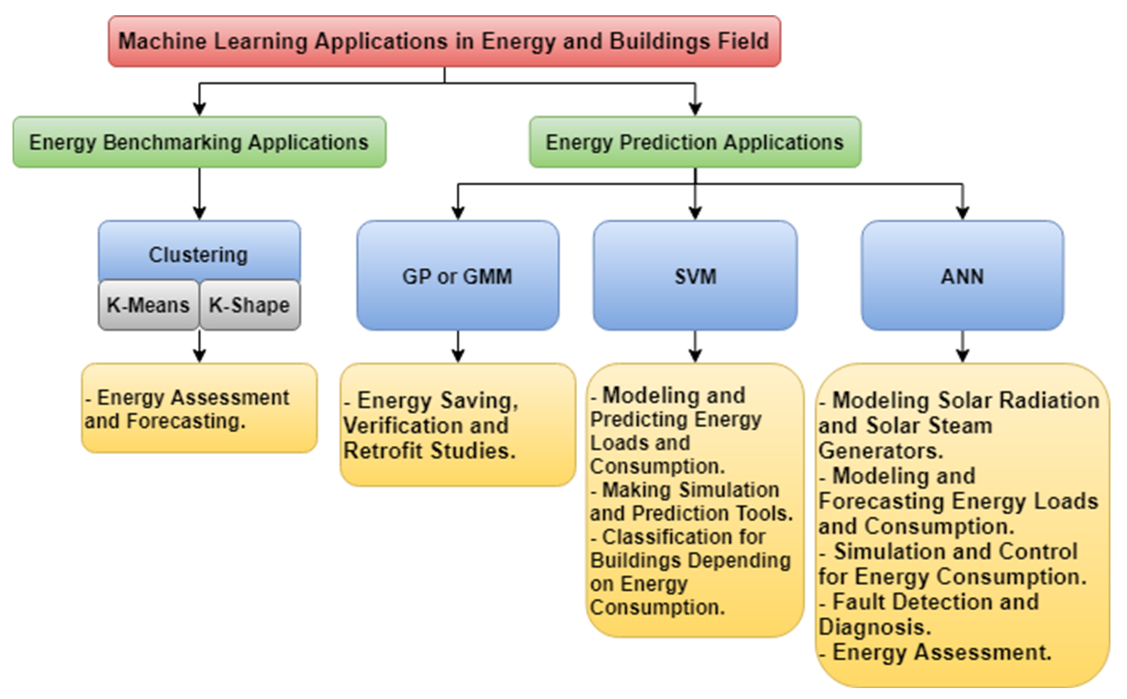
2.3. ML Algorithm Selection

In general, determining which machine learning algorithm is the best is difficult. As a result, it is critical to thoroughly examine the type of accessible or gathered data as well as the application to select the most appropriate model. The ML algorithm selection step depends on many factors such as (1) application-type factors and (2) data factors. In this section, applications of four ML algorithms (i.e., ANN, SVM, GPR or GMM, and Clustering K-Means or K-Shape) are explained to represent advantages, drawbacks, and potential improvements for each algorithm to help ML users in the selection process for the most appropriate algorithm during implementation in the field. After reviewing ML applications, the ML users in the energy and buildings field can deduce that (1) ANNs are a strong tool for modeling and reliable prediction of building energy. They do, however, need a careful selection of network topology and fine tweaking of their many hyper-parameters for training. Because ANN suffers from a local minimum issue, the models’ performance cannot be guaranteed. In addition, to obtain acceptable accuracy, ANN needs to be fed with a sufficient number of samples. Simple MLR models may be able to outperform them otherwise. As a result, ANN is best suited to engineers who are well-versed in deep learning and statistical modeling. We can also deduce that (2) SVM has been found to outperform ANN in load forecasting and can construct models from small data and (3) GPR is utilized for model training with uncertainty assessments among ML approaches and other black-box methods. Uncertainty and sensitivity analysis for various machine learning models have recently been presented and used. As a result, it is worthwhile to devote research resources to deploying these techniques for modeling construction under unclear data. Finally, we find that (4) in multi-dimensional energy assessment systems, k-means and k-shape are both highly efficient, with k-shape being used with time serious data and k-means being used with other data types. The popular applications of ML algorithms around the world in the field are explained in the following subsections and summarized in Figure 1.

2.3.1. Applications of ANN Algorithm

ANN algorithm represents a very powerful tool in the energy and buildings field because it can simulate the human brain by using nodes, weights, and layers to store information in parallel paths and it is extracted when necessary in a parallel way, too. This section demonstrates the ability of ANNs to be used in different applications of the energy and buildings field, with a description for implementation methods and contributions.

Modeling Solar Radiation and Solar Steam Generators

Kalogirou, in 1998, demonstrated several ANN applications in the field of solar energy. The author utilized artificial neural networks (ANNs) to predict solar radiation and a solar steam generator at varied incidence angles. ANN uses climatic parameters to estimate hourly solar irradiance in solar radiation modeling. ANN can forecast the collector intercept factor (i.e., the ratio of the energy absorbed by the receiver to the energy incident on the concentrator aperture) for solar steam generator design, as well as the radiation profile and the heat-up temperature response [41].

Modeling and Forecasting Energy Loads and Consumption

ANNs also take the place in energy simulation systems because they achieve fast computation time and performance in many applications. Olofsson et al. developed a long-term prediction and performance evaluation tool based on artificial neural networks (ANN) in 2001, using data from two to five weeks for six building families in Sweden built in 1970. The authors utilized the PCA approach to reduce the number of characteristics to only four (e.g., construction year, number of floors, framework, floor area, number of inhabitants, and ventilation system). The tool was created by using short-term data to evaluate performed retrofits and present conditions for improving the exited buildings, and made a long-term prediction for building energy consumption [20]. Ascione et al., in 2017, studied the ability to create a building energy prediction tool with low computational power and high accuracy. The tool was constructed using data from office buildings erected in southern Italy between 1920 and 1970. Based on the ANN algorithm, the authors presented two concepts of prediction tools: (1) used the existing data as it is, and (2) used the existing data but in the presence of energy retrofit measures. The proposed ANNs were optimized by “Simulation-based Large-scale sensitivity/uncertainty Analysis of Building Energy performance” (SLABE). The performances of the networks were estimated by using the distributions of the relative error to compare ANNs’ outputs with EnergyPlus program targets. The conclusion declares that the developed ANNs can replace standard building performance simulation tools, thereby reducing computational effort and time [42]. Beccali et al. studied EU non-residential building energy consumption in 2017 to develop an energy evaluation tool based on two artificial neural networks (ANNs), the first of which was used to forecast actual energy consumption and the second of which was used to assess economic indicators. The authors used 151 existent buildings in four locations of southern Italy to assess the two ANNs. The conclusion states that the decision support tool based on ANNs was able to forecast the energy performance of buildings quickly and accurately and that it was used to pick energy retrofit alternatives that can be implemented [43].

The ANNs’ flexibility is also declared in different applications when integrated with other optimization techniques to improve overall performance. Paudel et al. in 2014, integrated a pseudo-dynamic technique with an ANN model to make a daily short-term prediction for building heating demand. Because the hidden information in heating demand cannot be retrieved from climatic data by using ANN alone, the pseudo-dynamic approach improved the overall performance of the ANN model by aspects of operational heating power characteristics. The algorithm is used in the construction of French institutions. The created dynamic model is resilient, according to the conclusion, and may be utilized by energy service companies (ESCOs) in heat production dynamic control systems [44]. In 2017, Ascione et al. presented a detailed analysis and forecasting method based on ANN for cooling load of institutional building. For two years, data were collected from three institutional buildings. Due to the nature of vacation times and university timetables, the research reveals a large variance in daily cooling loads energy consumption. The authors proposed dividing the data into groups based on vacation times and university timetables to solve the problem of variation and examine it. The conclusion states that by adding categories’ numbers as a new input feature to the ANN algorithm, it was able to improve predicting accuracy. Furthermore, by utilizing the Bayesian regularization approach for the hyper-parameters automated tuning process, the performance of ANN can be most effective and rapid in computation time [45].

We can analyze the performance of the ANN algorithm declared in some previous papers to highlight the advantages and drawbacks by comparing it with other ML algorithms in the energy and buildings field. In 2015, Platon, Dehkordi, and Martel presented hourly electricity predictive models based on ANN and case-based reasoning (CBR) for an institutional building. The measured data from a Canadian institutional facility included elements, such as weather information, that are relevant to the building’s operation. To forecast power usage with a horizon of 1 to 6 h, the authors utilized principal component analysis to identify the most important characteristics (i.e., only 10 significant features were chosen out of 22 available features). The models’ prediction abilities were evaluated, and the ANN models regularly outperformed the CBR model, according to the results. Both the CBR and ANN models, on the other hand, had an error that was well within the ASHRAE limits. To improve the CBR model’s performance, different approaches were tried: (1) varying the case similarity criterion and the number of previous instances used for prediction and (2) using automated optimization techniques on values’ weight. However, none of these techniques had a substantial impact on the CBR models’ performance [15]. Edwards, New, and Parker, in 2012, sought to reduce difficulties such as a large number of features in the building characterization and prevent the problem of energy consumption in the predesign stage. The scientists used sensor-collected energy usage data to conduct statistical analysis using several machine learning methods (e.g., feed-forward neural network, support vector regression, least squares support vector machine, a hierarchical mixture of experts, and fuzzy c-means with feed-forward neural networks). To forecast next hour energy usage, researchers compared several machine learning algorithms on two types of data: (1) data on commercial building consumption gathered hourly and (2) data on residential building consumption collected every 15 min. According to the findings of this comparison, ANN-based techniques perform better on commercial structures. However, results show that these methods perform poorly on residential data and that least squares support vector machines perform best on both, but with high computation costs [18]. Kialashaki and Reisel, in 2013, created a hybrid method using artificial neural networks (ANN) and multiple linear regression techniques to forecast future energy consumption for residential buildings in the United States under various input scenarios (e.g., dwelling size, number of occupants, the efficiency of heating equipment and energy intensity). The authors describe how ANN’s effectiveness varies in residential structures in the United States, especially with test data. As the ANN model prediction is dependent on the cumulative trends of the various parameters, the reason for the variation in forecast energy was the fluctuation induced by the economic recession [19].

Simulation and Control for Energy Consumption

The energy consumption for buildings can be enhanced and controlled easily by using the ANN algorithm because it has the ability to deal with nonlinear equations in some applications. In 2015, Huang, Chen, and Hu proposed predictive control for an HVAC system to forecast an interior temperature by taking into account nonlinear building thermal dynamics (e.g., interaction between locations, noise in sensors, and delay time). Energy input from mechanical cooling, ventilation, weather, and convective heat transfers for thermal coupling between locations are all features of the ANN input. The suggested ANN model incorporates the thermal interaction between zones, resulting in more accurate prediction results than a single zone model, according to the conclusion. This management approach resulted in a high level of building energy consumption control [23]. In 2016, Benedetti et al. presented an automatic tool based on ANN to control building energy consumption and investigated the effect of the collected data period on the automatic utilization of such tools where a large amount of data is not always available in the real world, so the minimum and maximum period of required data were identified to achieve reliable results. To determine the optimal ANN design for an energy consumption management tool, the authors used three alternative ANN architectures. Furthermore, because a large quantity of data is not always present in practice, a method is presented for determining the minimum time of data collection required to achieve accurate findings and the maximum period of usefulness [46]. In 2017, Ahn, Cho, and Chung presented a hybrid control approach on mass and temperature for supply air of heating system to minimize energy consumption. To understand the nonlinear relations between features and forecast or assess precise thermal, the suggested technique uses a mix of fuzzy inference systems and ANN. To assess supply air conditions for a heating season, the suggested technique was compared to a basic thermostat on/off controller, and it was discovered that the ANN controller can reduce energy usage when compared to a simple thermostat on/off controller [47].

Fault Detection and Diagnosis

Time consumption problems during energy assessment and retrofit studies for buildings vanish in some studies. Kalogirou et al. proposed a fault diagnostic prediction system in 2008 that used temperature readings to identify problems in solar water heater components and forecast mistakes in collectors or pipe insulation. There were four elements to the problem diagnosis system: (1) a data acquisition system measured temperatures in four locations of the solar water heater system and the mean value for a storage tank; (2) a prediction module based on an artificial neural network (ANN) that was trained with fault-free system values obtained from a TRNSYS under the same meteorological conditions (e.g., Nicosia, Cyprus, and Paris, France), (3) the residual calculator takes measurement data from the data collection system as well as error-free predictions from the prediction module, and (4) the diagnosis module detects a variety of defects, including collector faults and insulation failures in the pipes linking the collection to the storage tank [48].

Energy Assessment

In 2013, Hong et al. studied the energy performance of schools (from 2008 to 2011) to create energy evaluations by combining statistical analysis with artificial neural networks (ANN) to evaluate the influence of each feature on energy and the relationship between them. About 7700 schools were utilized in a rapid statistical study, and 465 schools were investigated in depth using ANN to find variables that influenced school energy usage patterns. The results declared that the non-domestic buildings must be re-classified because of different reasons: (1) changes in the energy use pattern and (2) differences in energy performance between primary and secondary schools such as a gradual increase in electricity consumption and a decrease in heating consumption in both. By comparing simulation and engineering calculations, the authors noted the ability of ANN in energy assessment and the limitation in prediction [49]. Buratti, Barbanera, and Palladino developed a verification tool based on ANN in 2014 to forecast energy consumption and assess building performance by comparing it to energy certificates. The Umbria Region (central Italy) acquired around 6500 energy certificates (2700 of which were self-declarations). To train the ANN, the authors utilized only right certificates recognized by comparing them to energy standards, and they created a new index called the neural energy performance index to describe the degree of accuracy and to identify the certificate’s precise control needs (NEPI) [50].

2.3.2. Applications of SVM Algorithm

The SVM algorithm represents the best alternative solution for the ANN algorithm in many applications of the energy and buildings field. SVMs have a low number of hyper-parameters compared to ANN models, so they are easier to control and can be trained with small data sizes.

Modeling and Predicting Energy Loads and Consumption

The power and drawbacks of the SVM algorithm appeared in many applications of the field by comparing it with ANN models to solve the same problems. By using the SVM method for hourly cooling load forecast of an office building in Guangzhou, China, Li et al. demonstrated in 2009 that it is extremely successful, even with small data sets. The findings were compared to those of backpropagation ANN to indicate that SVM outperformed ANN in terms of accuracy and global solution. The input features were (1) outdoor dry bulb temperature of the past 2 h and (2) solar radiation intensity of the past 1 h. The result states that the SVM algorithm performed as well as the ANN method in terms of speed and accuracy, but with fewer data samples [28]. Using the least square support vector machine, Xuemei et al. increased the time efficiency required for hourly cooling load forecast in 2009 (LSSVM). The authors compared the proposed approach to backpropagation ANNs to assess its performance. In the end, LSSVM outperformed backpropagation ANN in terms of accuracy and global solution, especially when the available training set is restricted. As a result, LSSVM might be a viable option for predicting the cooling demand in a building [29].

After proofing the ability of SVM to replace ANN in different applications of the same field, there are different papers applied the algorithm with some adjustments to overcome drawbacks such as high time consumption when used with large data size. Hai Xiang Zhao et al. in 2009, studied the ability of SVM with the Gaussian kernel algorithm to deal with large time series datasets and reduce the training time of predicting energy models by using a concept of parallel SVM algorithms. Results showed very good performance in the prediction of energy consumption in multiple buildings based on large time series datasets [32]. Zhao and Magoulès, in 2012, studied the ability to reduce time consumption in SVM training with large data size by using radial and polynomial functions as a kernel for parallel SVM algorithms to predict the energy consumption of office buildings. The algorithm feature selection is implemented on data by using correlation analysis for features. Using correlation analysis for features, the algorithm feature selection is implemented on data. To compute the energy demands, the authors utilized simulated data from EnergyPlus software and manually selected features by computing correlation coefficients to reduce the number of features for the proposed algorithms [31].

Making Simulation and Prediction Tools

SVM algorithms can also outperform the ANN algorithm in dealing with residential buildings data for many cases such as energy prediction and creating tools. Jain et al., in 2014, used a support vector regression (SVR) algorithm with sensor measurements from residential buildings to make energy predictions. The inputs feature during training were (e.g., weather, time of day, and previous energy consumption) from multi-family residential building data in New York City. The authors mentioned a paucity of research applying multi-family residential buildings. Thus, he expanded the study-to-study algorithm limitations by examining different time steps (i.e., 10 min, daily, and hourly) and different spatial categories (i.e., by unit, by floor, and whole building). The conclusion declares that the SVR could be used in energy prediction for residential buildings and the best prediction results occurred at floor level in hourly intervals [30]. In 2008, Lai, Magoulès, and Lherminier utilized SVM to develop a simple and rapid method for predicting the electric energy consumption of residential buildings. The data include daily electricity usage for a year and three months, as well as climatic data such as temperatures and humidity. For the learning stage, the authors utilized a year and two months, and for the prediction step, the authors used the last month. The findings demonstrate that the model has high performance and that the SVM tool may be utilized to conduct predictive modeling [51].

Classification for Buildings Depending on Energy Consumption

The SVM algorithm is very flexible to be integrated into existing systems on building energy management. In 2010, Li, Bowers, and Schnier developed a daily power consumption management system for buildings based on detecting abnormal energy behavior and providing the capacity to handle problems in real time to enable prediction and detection of abnormal energy usage. The system consisted of the following steps: (1) outliers’ detection in real time to identify abnormal energy use and delete it from further analysis, and (2) classifying based on the SVM-predicted daily electricity profile. The suggested system was computationally efficient and resilient enough to be incorporated into current building energy management and alarm systems [52].

2.3.3. Applications of GPR or GMM Algorithm

Energy Saving Verification and Retrofit Studies

Although the Gaussian-based algorithms need high computation power resources, they have a lot of advantages declared through implementation in some complicated applications which make them used in the field. In 2012, Heo and Zavala investigated the possibility of the GPR model to substitute a linear regression approach in energy savings, uncertainty measurements, and verification problems since it is highly powerful in prediction, particularly with noisy data. The conclusion asserts that generalized linear models (GPR models) can represent complicated behavior (i.e., nonlinearities, multivariable interactions, and time correlations). Furthermore, because they were created in a Bayesian environment, they can overcome difficulties of uncertainty [33].

These solution algorithms are best in the case of noisy data or probabilities and retrofit studies to help decision makers in taking steps in improving countries. Furthermore, in 2012, Heo, Choudhary, and Augenbroe presented a scalable, probabilistic methodology for energy modeling based on Bayesian calibration (the same base for Gaussian models) to improve modeling by detecting uncertainty in buildings models and aid in studying the probability of building energy consumption improvements and retrofit performance. The suggested technique, according to the conclusion, may accurately assess energy retrofit choices and promote risk-aware decision-making by clearly inspecting risks associated with each retrofit option [35].

The GPR and GMM algorithms can be integrated with other models to improve performance even if the collected data are limited. In 2014 Burkhart, Heo, and Zavala utilized a GPR with a Monte Carlo expectation maximization (MCEM) model to cope with noisy data from sensors (e.g., weather, occupancy) and investigated the impact of the method on the quantity of necessary data from sensors during measurement and verification (M&V) stages. The GPR-MCEM model, according to the result, reached robust prediction levels when compared to conventional GPR alone, and may be utilized as a mechanism to decrease data collection and sensor installation costs in M&V processes since it provides high performance with fewer data [34].

2.3.4. Applications of Clustering Algorithms (K-Means and K-Shape)

Energy Assessment and Forecasting

The benchmarking process is very helpful in building energy assessment applications, especially when integrated with other algorithms to create energy assessment techniques. In 2007, Santamouris et al. developed an intelligent technique to cluster school buildings as the first step in energy assessment procedures. Then, the output clusters used in the energy performance studies specified the buildings’ rating and environmental impact of each cluster. The energy rating of the school buildings gives detailed information on their energy consumption and efficiency in comparison to other buildings of a similar kind, allowing for better intervention planning to enhance their energy performance. The authors created the technique in three steps: (1) energy consumption data were collected from 320 schools in Greece, (2) fuzzy clustering techniques were used to make the energy rating scheme, and (3) 10 schools were selected and detailed analysis was performed for energy efficiency, performance, and environmental impacts. The conclusion declares the ability of the used technique to identify and rate the existing school buildings and studied the potential for energy and environmental improvements [39]. Gaitani et al., in 2010, presented an energy classification tool for school buildings’ heating based on a k-means clustering technique with PCA to help decision makers in the schools rating process and study probabilities of energy savings. The data used consisted of 1100 cases from secondary education school buildings in Greece, which represented 33% of the total secondary school sector, and included information such as energy consumption for space heating and lighting, building area, number of students and professors, a boiler installed power, building manufacturing year, and operation schedule. The tool was created in three steps: (1) an extensive statistical analysis on the data was performed, (2) PCA was applied to select the most significant features, and (3) a k-means clustering technique was used to classify. The results state that the categorization may be used to aid decision makers’ energy-saving strategies [40]. In 2017, Yang et al. proposed an energy clustering method based on the k-shape algorithm for time series data, which can recognize patterns in time series data and categorize them using multi-dimensional space. The clustering was performed on data from 10 institutional buildings’ hourly and weekly energy usage using the k-shape method to find form patterns in time series data, which increased the accuracy of forecasting models. The conclusion declared that the proposed method could detect building energy usage patterns in different time intervals effectively and also proved that the forecasting accuracy of the SVR model is significantly improved by integrating the clustering method with the SVR model [36].

These clustering algorithms also prove efficiency as an alternative solution for software such as the Energy Star program. In 2014, Gao and Malkawi proposed a benchmarking technique based on the smart clustering concept, which classifies buildings’ energy based on all features that have a relationship with energy consumption and groups buildings with the most similarity of features into one cluster, implying that the problem of classifying is multi-dimensional. The proposed methodology contains four steps: (1) data collection, (2) feature identification and selection, (3) selection for clustering algorithm depending on collected data, and (4) buildings’ benchmarking concerning cluster group and centroid. The findings were compared to the Energy Star approach to show that the suggested strategy can give a more thorough approach to benchmarking, particularly with multi-dimensional challenges, inspiring a fresh viewpoint on building energy performance benchmarking [37].

The complexity of ML problems can be handled by the clustering algorithms, which convert the chaos data to more homogenous ones in simple iterative steps. Arambula Lara et al. in 2015, studied the European policy of energy saving and the Commission Delegated Regulation (EU) 244/2012, which gave recommendations for some reference buildings to make a compromise cost from expected improvements. The solution was found in the k-means clustering approach, which split huge data into tiny and homogeneous groups based on building characteristics’ similarity, decreasing the complexity of energy optimization and retrofits by reducing school buildings’ stock homogeneously. The data came from a sample of roughly 60 schools in the region of Treviso in northern Italy, collected between 2011 and 2012. The conclusion declares that this method could identify a small number of parameters to assess the energy consumption for air heating and hot water production [38].

2.4. Model Training, Validation, and Tuning

This is an iterative process during the conversion of a solution that can be performed many different times. Initially, upon training, the model will not achieve the results that are expected. Thus, the tuning process is very important to evaluate model performance under different values of hyper-parameters. During training, the machine learning algorithm updates a set of numbers known as parameters or weights. The goal is to update model parameters in the global solution direction which makes the predicted output as close as possible to the true output (as seen in the data). This cannot be achieved in one iteration, because the model has not yet learned; it watches the weights and outputs from previous iterations and shifts the weights to a direction that lowers the error in the generated output. If the error in the output gradually decreases with each successive iteration, the model is said to converge, and the training is considered successful. If, on the other hand, the errors either increase or change randomly between iterations, the hyper-parameters of the model need to be tuned [12].

The most important thing in model performance is overfitting and underfitting. The underfitting problem means that the model performance is very low on the training data, and thus, the training model is unable to represent the data correctly. In underfitting problems, the model could be very simple (the problem cannot be formulated well with enough features) to produce accurate outputs well, because of the inability to extract patterns or relationships between input and output features for data. To overcome the underfitting problem, there are different techniques: (1) reformulate the real-life problem by adding more effective features, (2) choose suitable preprocessing methods to solve data drawbacks of missing or outlier values, and (3) decrease or change amount or type of model regularization techniques such as dropout. The problem of overfitting is present when the model performance is very high on training data but low on the validation or test data. The reason for the overfitting problem is the inability of the model to attain the global solution of the problem to cover all data sets. With low performance for unseen data, it makes sense to use fewer feature combinations and increase the amount of regularization [53].

There are several techniques to overcome overfitting and maximizing generalization. The most popular one is simple Hold-Out Validation. The simple hold-out technique depends on splitting data into multiple sets for training, validating, and testing models. Training data, which include both features and labels, feed into the model. The model is then used to make predictions over the validation data set, which checks performance to tune and change the model’s weights. Then, test data that only include features are used to produce the labels. The performance of the model with the test data set is what we can reasonably expect to see in real life [13,54,55].

The problem of the hyper-parameters tuning process is mainly related to the ML algorithm type. For the ANN algorithm, many papers discussed this problem during the implementation of different real-life problems and recommended using an automatic technique in the tuning for a large number of ANN hyper-parameters because the ANN model has a lot of hyper-parameters.

González and Zamarreño, in 2005, studied the effect of hyper-parameters such as the number of neurons per layer and data size on the performance of ANN while creating an algorithm for short-term building load prediction. The authors mentioned difficulties in reaching the global solution because it related to large numbers of ANN hyper-parameters values [25]. Dombaycı et al. in 2010, studied the number of neurons per layer only as a hyper-parameter for an ANN model that was developed to make an hourly heating energy prediction in the design stage for a building to help in selecting appropriate and efficient heating and cooling equipment. The authors explained the complexity of tuning ANN hyper-parameters by using manual methods because of their large numbers [13]. One of the trials to overcome the problem of a large number of hyper-parameters was conducted in 2015 by Li et al., who used particle swarm optimization technique in automatic ANN hyper-parameters tuning while improving the short-term building hourly electricity consumption prediction and compared this method and simple ANN with manual tuning for hyper-parameters. The authors concluded that the automatic tuning process has a shorter training time and higher performance than the manual method and the hybrid genetic algorithm model [16]. In 2017, Ascione et al. presented a solution for the same problem using the Bayesian regularization technique for hyper-parameters’ automatic tuning while making a detailed analysis and forecasting method based on ANN for the cooling load of institutional buildings, and mentioned that the performance of ANN is the most effective and quick in computing time by using this tuning technique [45].

Otherwise, the SVM algorithms are easily tuned and manually optimized. These advantages appeared in many applications such as in 2009 when Zhijian Hou et al. studied the ability to replace huge numbers of trainable parameters for ANN by using radial function as a kernel for an SVM algorithm in an HVAC system energy prediction in Nanzhou. The paper proved that the algorithm has fewer parameters to tune compared with ANN and is better than the ANN algorithm in forecasting [27].

2.5. Model Evaluation

The model evaluation is performing using test data to make sure that the required goal is achieved and to overcome the problem of over-fitting and under-fitting for the trained model. If the trained model does not meet the required goal, it increases the required time to re-validate the model and achieve goal. In this step, the feature engineer takes the role to study data and features and find ways to improve the model, and the way that it is produced. Once the retraining happens and the required goal is achieved, the model is deployed to perform the best possible predictions on the unknown data to begin evaluating how the model responds in a non-training environment.

To evaluate the machine learning model, we need to know the type of ML problems, classification (such as benchmarking), or regression (such as prediction) problems. The type of machine learning problem will influence the type of metric used to evaluate the model. We can start by looking at classification problems metrics. There are different types of metrics to evaluate models: (1) accuracy, (2) precision, (3) recall, (4) F1 score (2*(recall*precision)/(recall + precision)), and (5) area under the curve-receiver operator curve (AUC-ROC). To implement this metric method on the trained model, the model predictions and the known target values are sent to the confusion matrix. A confusion matrix is the building block for running these types of model evaluations for classification problems. Then, the predictions are returned, compared with the values of ground truth. Finally, the evaluation metric between predicted values and ground truth values is computed [56].

It is recommended in classification problems to use F1 as an evaluation metric because the F1 score combines precision and recall together to give one number to quantify the overall performance of a particular ML algorithm. In addition, the F1 score should be used when the dataset has a class imbalance but we want to preserve the equality between precision and recall.

In regression problems, there are other common metrics that we can use to evaluate the model: (1) mean squared error and (2) R-squared. Mean squared error is very commonly used. The difference between the prediction and actual value is calculated, that difference is squared, and then all the squared differences for all the observations are summed up [16].

The other metric type is R-squared, which explains the fraction of variance accounted for by the model. It is like a percentage, reporting a number from 0 to 1. When R-squared is close to 1, this usually indicates that a lot of the variabilities in the data can be explained by the model itself. The threshold for a good R-squared value depends on your machine learning problem. In some machine learning problems, it is very difficult to achieve a high R-squared value. The high value of R-squared does not always represent strong model performance because R-squared is always increasing when more variables are added to the model, which sometimes leads to overfitting [13]. To counter this potential issue, there is another metric for model performance called the Adjusted R-squared value. The Adjusted R-squared has already taken care of the added effect for additional variables and it only increases when the added variables have significant effects on the prediction. The adjusted R-squared adjusts the final value based on two factors: (1) the number of features and (2) the number of data points in the data. A recommendation, therefore, is to look at both R-squared and Adjusted R-squared. This will ensure that the model is performing well but also that there is not too much overfitting.

In the building energy prediction field, it is preferred to evaluate ANN using mean absolute percentage error (MAPE) as a performance metric during model training. It is used in different applications in the same field and is proved to be very effective in the examination of model quality during the prediction process [25].

The most recommended evaluation technique is the cross-validation method that was used in 2006 by Karatasou, Santamouris, and Geros. They evaluated the hourly buildings load predictor based on feed-forward artificial neural network (FFANN) by splitting the data into many packages and looping them in the training process (i.e., each iteration in the training process carried out by using one of the packages as test data and others as training data to cover all data samples without overfitting problems). In addition, the authors discussed the cross-validation technique effect during training on the result of prediction and modeling and recommended this technique in such applications to achieve more robust models. The authors also discussed, the importance of attaining a more robust model by using different types of data sets in the evaluation process (i.e., the model performance was evaluated using two different data sets: (1) energy prediction shootout I contest and (2) an office building in Athens) [21]. Furthermore, one of the evaluation techniques was used by Dombaycı et al. in 2010 while developing an hourly heating energy prediction model based on ANN for building. The total data of 35,070 h were split into two packages to train and test the model: (1) the data from 2004 to 2007 (i.e., 26,310 data sample) used during model training, and (2) the data of the year 2008 (i.e., 87,60 data sample) used in model testing or evaluating. The authors mentioned the importance of using test or unseen data to improve model performance in real life [13].

2.6. Model Verification

The verification of machine learning models’ robustness refers to checking models deployed on a real-life problem to ensure that it adheres to these specifications and achieves the target for a long run. A variety of machine learning models are also assessed according to how robust they are proven to be. This step must be performed frequently to make sure that the system is still working in high performance.

The evaluation step represents the base for verification steps during model deployment. The more models are robust in the evaluation step, the easier the verification step, and results in real life will be better. The robustness or verification for any model is examined firstly during the evaluation step by using unseen data or new data that differed from training data. Different types of data packages in many applications are used in the ML model evaluation step, such as in the 2006 work Karatasou, Santamouris, and Geros, who evaluated the FFANN models by using two different data sets: (1) energy prediction shootout I contest, and (2) an office building in Athens. In addition, they trained models on different time steps to identify limitations for models and create a robust hourly buildings load predictor tool so that the FFANN can be deployed on different data sets and used for a long run [21]. Moreover, in 2015, Li et al. collected hourly data from two resources: (1) energy prediction shootout contest I, and (2) a campus building in east China; meaning that the data were collected from different locations all over the world to ensure the reliability and robustness of the model [16].

3. Discussion

As shown in Figure 2, the generic ML covers all required steps to use and deploy the ML algorithms (i.e., ANN, SVM, GPR or GMM, and k-mean or k-shape clustering) in the energy and buildings field. The pipeline starts with problem identification (i.e., identify application type and specify the benchmarking and prediction problems). Then, this real-life problem must be converted to an ML problem in the problem formulation step by identifying the related features. After that, the data scientists start in collecting the data depending on the related features identified in the previous step and make some statistical analysis and visualization to study the nature of collected data and their distribution (this step is very important to help data scientists in choosing the appropriate preprocessing techniques).

Thereby, the data preprocessing step starts with answering some questions: (1) are there too many features? If there are too many features, the features must be decreased by feature selection (i.e., keeping only the most significant features that have a high effect on the studied problem). If there are not too many features, the second question is (2) are there too few features? If the collected data have a small number of features that have nonlinear or deep interaction relationships, the data scientist must employ some feature extraction techniques to increase the number of features and help the algorithm reach for a global problem solution during training. The third question concerns (3) noisy data. If the data contain noise, the filtration must be carried out by Gaussian based models or the Kalman filter. The fourth question concerns (4) time series data. To identify the noise filter type, this question must be answered to select between Gaussian-based models or the Kalman filter. The final step in preprocessing steps is solving problems of outliers and missing values.

Then, the most appropriate ML model must be selected. The selection depends on the ML problem type (i.e., benchmarking or prediction) that is identified in the first step in the proposed pipeline. In addition, some questions must be answered to identify the algorithm type. The first question concerns (1) time series data. If the data are time series, the k-shape clustering algorithm is the best selection for benchmarking. If not, the k-means clustering algorithm is better. The second question concerns (2) very big data. If the data are very big, the ANN algorithm is the best solution for prediction problems. If not, the next question concerns (3) complex systems. If the data have nonlinear or deep interaction relationships between features, the GPR or GMM are the best solution models for prediction problems. If not, the SVM model is better. After that, the labels from clustering is appended to the data in benchmarking to analyze the result, and the data must be normalized before training in prediction problems.

Then, the model is trained, validated, tuned, and evaluated by using the cross-validation technique to create a robust model. Finally, if the evaluation results achieve the model goal, the model is deployed in real-life applications and make verification processes regularly. If the results are bad, the feature engineering must be conducted to increase or decrease features more and more (i.e., feature selection or feature extraction) and return to the training step again, or the collected data are not enough and must be increased by a return to the problem formulation again.

The final ML pipeline is very important for ML users in the energy and buildings field because it abbreviates a high level of experience in one pipeline to avoid the time consumption from new ML users to learn the potential of each ML algorithm. For more demonstration, we explain some previous work in the field by using the proposed pipeline (in

Table 1. Review of some previous papers comparing them with the proposed ML pipeline.

Preprocessing Questions and Actions							Model Selection Questions and Actions						Model Creation
Too Many Features? or Too Few Features?	Extracted or Selected Features	Noisy Data?	Time Serious Data?	Kalman or Gaussian Filters	Outliers’ Values	Missing Values	Benchmarking or Prediction?	Time Serious Data?	Very Big Data?	Complex System?	Selected Algorithm?	Append Clusters Labels to Data? or Normalize Data?	Training, Validation and Tuning	Evaluation
Not asked	-----	×	√	-----	-----	removed	prediction	√	√	Not asked	ANN	normalized	Applied cross-validation on two data sets	Used two data sets and tried different samples steps	[21]
Not asked	-----	×	√	-----	-----	-----	prediction	√	√	Not asked	ANN	normalized	Split data to train and test sets	Used test data	[13]
Too many features	Selected features using correlation between features	√	√	-----	Keep as it	Keep as it	prediction	√	√	√	ANN	normalized	Split data to train, validate, and test sets with different samples steps	Used test data with different samples steps	[57]
Too many features	Selected features using PCA	×	√	-----	-----	-----	prediction	√	√	Not asked	ANN	normalized	Split data to train and test with automatic tuning (PSO)	Used test data	[16]
Too many features	Extracted features using k-shape clustering	√	√	-----	Filtered	Imputed	Benchmarking and prediction	√	Not asked	Not asked	k-shape and SVM	normalized and append cluster labels	Split data to train and test and applied cross-validation	Used test data with different samples steps	[36]
Not asked	-----	√	√	-----	-----	-----	prediction	√	√	√	GPR	normalized	Split data to train and test with different samples steps	Used test data with different samples steps	[33]
Too many features	Selected features using p-value	×	√	-----	-----	replaced	Benchmarking	×	√	Not asked	k-mean	normalized	Applied similarity measure on one package data	Compare results with EnergyStar software	[37]

and

Table 2. The details of the reviewed papers and the comments that result from comparison with the proposed ML pipeline.

Model Target	Data Source	Data Size	Model Features	Selected Algorithm?	Best Evaluation Results	Comments and Expected Improvements
Predict Hourly Energy Consumption [21]	“Two different data sets provided from two different buildings: The first set is the benchmark PROBEN 1, and comes from the first energy prediction contest, the Great Building Energy Predictor Shootout I, organized by ASHRAE (data set A) & The second data set derives from an office building located in Athens, Greece (data set B)”	data set A: a total of 4208 time steps, data set B: a total of 8280 time steps	data set A: “temperature, solar radiation, humidity ratio and wind speed” data set B: “ambient temperature, humidity, daily, weekly and yearly cycles the hour of day, day of week and day of year”	ANN	data set A: RMS is 15.25, MAPE is 1.50, CV is 2.44 and MBE is 0.37 data set B: RMS is 1.13, MAPE is 2.64, CV is 2.95 and MBE is −0.03	There are some wrong prediction peaks due to ignoring the effect of the outliers in preprocessing data step, and the evaluation would be better if carried out on the same model structures with different data sets but with the same input features to increase reliability and robustness.
Predict Hourly Heating Energy [13]	“A model house designed in Denizli which is located in Central Aegean Region of Turkey”	A total of 35,070 time steps	“Month, day of the month, hour of the day, and energy consumption values at certain hours”	ANN	RMSE is 1.2125, R2 is 0.9880 and MAPE is 0.2081	The author did not mention any preprocessing steps, just normalization because the used data was calculated, which did not have the same worth of actual data, and the trained model could be more robust if the cross-validation technique was used in training and different time steps during the evaluation,
Predict Hourly Energy Consumption [57]	“CIESOL bioclimatic building, located in the southeast of Spain”	A total of 700,000 time steps	“The type and hour of the day, weather variables (outdoor temperature, outdoor humidity, solar radiation, wind velocity and wind direction) and the state of the actuators from the solar cooling installation”	ANN	Mean error is 11.48%	Although the authors mentioned the outliers and noise in the data, they did not apply any type of analysis to solve these two problems in the data. In addition, the missing values in the data are kept as is and the authors depended on a manual method in splitting data to skip missing values, which means the splitting blocks are imbalanced. Therefore, the efforts made in the training and evaluation steps to create a robust model were useless because the preprocessing steps are not well performed, so the results from the model have a relatively high mean error.
Predict Hourly electricity consumption [16]	“The Great Building Energy Predictor Shootout I, organized by ASHRAE in 1990s (data set A) Data from a library building located in Hangzhou, East China (data set B)”	data set A: a total of 4208 time steps, data set B: a total of 2472 time steps	Data A: “outdoor dry bulb temperature, solar radiation, humidity ratio and wind speed” Data B: “daily temperature and occupancy”	ANN	data set A: CV is 0.0254 and MAPE is 0.0162 data set B: CV is 0.0758 and MAPE is 0.058	The authors did not mention anything about the missing values in the data. The automatic tuning gives high prediction results, but it needs to integrate with a cross-validation technique to ensure the robustness and reliability for model.
Benchmark and predict (hourly and weekly) Energy consumption [36]	“10 institutional buildings in Singapore”	a total of 122 days for each building	“Hourly and weekly energy consumption”	k-shape and SVM	Respective MAPE values are 15.36, 9.46, 1.033 1.23, 2.37, 3.66, 0.57, 54.11, 3.63, 4.46 for the ten buildings	The authors mentioned the noise in data but did not mention solving it. In addition, the outliers and missing values did not mention solve in the technique. The data size is relatively high to be used in SVM algorithms (the authors did not take into consideration the data size when selecting the algorithm), and the authors extracted features to decrease complexity and effort. Thus, it is recommended to used parallel SVM to reduce time.
Predict Daily Energy Performance [33]	“Real weather data in the Chicago area”	a total of 8736 time steps	“Weather and occupancy levels, and the most commonly used is outdoor dry-bulb air temperature”	GPR	SSE is from 2.7e5 to 3.6e6 and total energy savings prediction error is from 31 to 41.23	The data size is relatively large, and the authors did not mention time consumption in training, as it may be too large. Therefore, it will be better to use the Gaussian model to remove noise only and complete prediction by ANN or use ANN directly for all problems.
Benchmark annual Energy Performance [37]	“commercial building (CBECS database)”	5215 samples	“Area, percent heated, percent cooled, wall materials, roof materials, window materials, window percent, shape, number of floors, construction year, weekly operation hours, occupants, variable air volume, heating unit, cooling unit, economizer, refrigerators, number of servers, office equipment, heating and cooling degree day”	k-mean	Ratio between actual energy index to centroid for cluster in range from 0.96 to 2.1 for each cluster	The data contain outliers, but the authors did not mention this or the technique to solve this. In addition, the imputation for missing values is not declared well. The evaluation step is carried out using a comparison with EnergyStar without declaration of any approach to overcome the local minimum solution of the k-mean algorithm.

) to prove that the pipeline can be used as a reference for implementing the ML concept in the right way and achieving high performance:

(1)

In 2006, Karatasou, Santamouris, and Geros designed an hourly buildings load prediction tool based on a feed-forward artificial neural network (FFANN). By comparing between paper steps and the proposed pipeline, it is found that the authors did not mention any preprocessing steps except statistical analysis. They stated that the data did not have any noise, removed the missing values, and normalized the data. Thus, they did not take the full benefits of statistical analysis to study the data nature, and there are some wrong prediction peaks due to ignoring the outliers’ effect in the preprocessing data step. Because of the large data size and since the ML type is prediction, the selected algorithm was ANN, and they implemented the cross-validation technique to create a robust model. In addition, the ANN algorithm was evaluated with two different data sets to ensure robustness, but it is not enough because the evaluation would be better if performed on the same model structures with different data sets but with the same input features to increase reliability and robustness [21].

(2)

Dombaycı et al., in 2010, developed an hourly heating energy prediction model based on ANN to estimate energy in the design stage. The authors did not mention any preprocessing steps, just normalization, because the user data were calculated, so the probability of containing noise, missing values, and outliers is very small (this does not have the same worth of actual data). The ANN was used because the data are big and the ML problem concerns prediction. The data were split to train and test sets, but this was not enough because the trained model could be more robust if the cross-validation technique was used in training and evaluation steps [13].

(3)

Mena et al., in 2014, developed and assessed a short-term predictive ANN model of electricity demand. The authors manually reduced the number of features because the data had a high number of features. Although the authors mentioned the outliers and noise in the data, they did not apply any type of analysis to solve these two problems in the data. In addition, the missing values in the data are kept as is and the authors depended on a manual method in splitting the data to skip missing values, which means the splitting blocks are imbalanced. Thus, the efforts made in the training and evaluation steps to create a robust model are useless because the preprocessing steps are not well performed, so the results from the model have a relatively high mean error [57].

(4)

In 2015, Li et al. improved the short-term hourly electricity consumption prediction of a building. The authors mentioned a large number of features, so they used an automatic method of reducing features (PCA). However, the authors did not mention anything about the missing values and outliers in the data. Because of the large data size and since the ML type is prediction, the selected algorithm was ANN. The automatic tuning gives high prediction results, but it needs to integrate with cross-validation techniques to ensure the robustness and reliability of the model [16].

(5)

In 2017, Yang et al. proposed an energy clustering and prediction method based on k-shape and SVM algorithms for time series data. The authors mentioned the noise in the data but did not mention solving it. In addition, there was no mention of any technique to solve the problem of outliers and missing values. The data size is relatively high to be used in SVM algorithms (the authors did not take into consideration the data size when selecting the algorithm), and the authors extracted features to decrease complexity and effort during model training. Due to the huge data size, it is recommended to used parallel SVM to reduce time or replace it directly with ANN [36].

(6)

Heo and Zavala, in 2012, used the GPR model in energy savings and uncertainty measurements and verification problems. The authors did not use any feature extraction concept, although they mentioned a high degree of complexity in the data due to noise and nonlinear relationships. Moreover, they did not mention any technique to detect and solve the outliers and missing values problems. The data size is relatively large and since the authors did not mention time consumption in training, it may be too large. Thus, it will be better to use the Gaussian model to remove noise only and complete the prediction by ANN or use ANN directly for all problems [33].

(7)

In 2014, Gao and Malkawi proposed a benchmarking technique for building energy based on the k-means concept. The authors used the features selection technique due to the high number of features. The data contain outliers, but the authors did not mention the technique to solve this. In addition, the imputation technique for missing values was not declared well, which greatly affected the k-means solution (the k-means has a high probability of falling into local minimum) [37].

4. Implement the Pipeline on CBECS Data

In this section, the pipeline is used as a reference to make commercial building energy predictions by using CBECS data. The data are collected by the US Energy Information Administration (EIA). Since 1979, the EIA has performed the CBECS regularly, as mandated by Congress. For commercial buildings, the EIA gathers data in two parts: (1) building characteristics or features are gathered through an in-person or online survey of building owners and managers, and (2) energy use data are gathered from power suppliers.

After collecting the data, the preprocessing and visualization step follows. The targets during data visualization are to (1) check missing values, (2) check outlier values, and (3) understand the nature of each feature distribution (normal distribution or skewed distribution). The visualization helps to choose the best method suitable for filling missing values and replacing outlier values. The difference between mean and median reflects the influence of outliers on data distribution, as seen by the calculation procedure of mean and median values for each characteristic in

Table 3. Selected features’ characteristics.

Selected Features	Values and Ranges Format	Analysis before Changes	Notes and Changes	Analysis after Changes
Square footage (SQFT)	1001–1,500,000	Mean = 124,473.50 Median = 20,750.00 Std = 258,613.18 Outliers = 12.31% Missing = 0.0%	No changes	Mean = 124,473.50 Median = 20,750.00 Std = 258,613.18 Outliers = 12.31% Missing = 0.0%
Number of floors (NFLOOR)	1–14 994 = 15 to 25 995 = More than 25	Mean = 30.16 Median = 2.00 Std = 163.61 Outliers = 9.73% Missing = 0.0%	Change (994 = 15 to 25) to (‘20’ = 15 to 25) as mean value to this range and change (995 = More than 25) to (30 = More than 25) [17]	Mean = 3.01 Median = 2.00 Std = 4.31 Outliers = 9.73% Missing = 0.0%
Year of construction (YRCON)	995 = Before 1946 1946–2012	Mean = 1861.10 Median = 1981.00 Std = 325.77 Outliers = 12.37% Missing = 0.0%	Change (995 = Before 1946) to (1932 = Before 1946)	Mean = 1976.97 Median = 1981.00 Std = 23.34 Outliers = 0.00% Missing = 0.0%
Total hours open per week (WKHRS)	0–168	Mean = 78.02 Median = 60.00 Std = 51.37 Outliers = 0.00% Missing = 0.0%	No changes	Mean = 78.02 Median = 60.00 Std = 51.37 Outliers = 0.00% Missing = 0.0%
Number of employees (NWKER)	0–6500	Mean = 178.78 Median = 15.00 Std = 565.94 Outliers = 15.97% Missing = 0.0%	No changes	Mean = 178.78 Median = 15.00 Std = 565.94 Outliers = 15.97% Missing = 0.0%
Percent heated (HEATP)	0–100 Missing = Not applicable	Mean = 88.52 Median = 100.00 Std = 24.24 Outliers = 19.94% Missing = 7.75%	Fill missing values with 0 because (not applicable mean zero percentage)	Mean = 81.49 Median = 100.00 Std = 33.38 Outliers = 15.73% Missing = 0.0%
Percent cooled (COOLP)	1–100 Missing = Not applicable	Mean = 79.81 Median = 100.00 Std = 30.13 Outliers = 8.29% Missing = 10.18%	Fill missing values with 0 because (not applicable mean zero percentage)	Mean = 71.68 Median = 95.00 Std = 37.39 Outliers = 0.00% Missing = 0.0%
Number of computers (PCTERMN)	0–4195 Missing = Not applicable	Mean = 168.93 Median = 10.00 Std = 530.48 Outliers = 16.21% Missing = 3.56%	Fill missing values with 0 because (not applicable mean zero)	Mean = 162.92 Median = 9.00 Std = 521.90 Outliers = 16.1% Missing = 0.0%
Percent lit when open (LTOHRP)	0–100 Missing = Not applicable	Mean = 82.12 Median = 95.00 Std = 25.01 Outliers = 8.04% Missing = 4.4%	Fill missing values with 0 because (not applicable mean zero)	Mean = 78.50 Median = 90.00 Std = 29.70 Outliers = 8.66% Missing = 0.0%
Annual electricity consumption (thous Btu) (ELBTU)	Output Feature	Mean = 9,283,680.98 Median = 822,346.50 Std = 32,174,631.57 Outliers = 14.67% Missing = 2.47%	No changes	Mean = 9,283,680.98 Median = 822,346.50 Std = 32,174,631.57 Outliers = 14.67% Missing = 2.47%

. In addition, the visualization of missing values of each feature is very important to decide which feature is suitable to be taken in the training of ML because features with a high percentage of missing values cannot be taken.

The first question in the pipeline comes after the preprocessing and visualization step (i.e., do the data have a high number of features?). The data contain a large number of features, so the feature selection step must be implemented to select the most significant features. The features selection step depends on the paper [17], which depended on calculating linear correlations between studied features and selecting the most appropriate ones (i.e., have a low level of missing values and high correlation with output features). The selected features are (‘Square footage’, ‘Number of floors’, ‘Year of construction’, ‘Total hours open per week’, ‘Number of employees’, ‘Percent heated’, ‘Percent cooled’, ‘Number of computers’, ‘Percent lit when open’, ‘Annual electricity consumption (thous Btu)’).

By moving through the pipeline, the answer to the next question (i.e., are the data noisy?) leads to the final part in the preprocessing steps (i.e., solving the problems of missing values and outliers). These problems are primarily declared through the visualization step for features. There are missing values and outliers in some features, so some changes are made (shown in Table 3) as a first action to reduce these effects during ML model training. After making these changes, the missing values are eliminated in all features except the ‘Annual electricity consumption (thous Btu)’ feature, which still has a small percentage of missing values that can be replaced by the median value of the feature. In addition, the percentage of outliers’ values decreased significantly but was not eliminated.

The remaining outliers’ values can be decreased by combining two features or more in one feature to reduce the effect of very high and very low values in each feature on the model. The final features are (‘Total hours open per week’, ‘Building age’, ‘Building area per employee’, ‘Building area per PC’, ‘Building area per employee’, ‘Number of floors’, ‘Percent heated’, ‘Percent cooled’, ‘Percent lit when open’, and ‘Electricity use per area’). The new features’ analysis shows that the new features (

Table 4. The final features of the ML model.

Selected Features	Analysis before Changes	Notes and Changes	Analysis after Changes
Total hours open per week	Mean = 78.02 Median = 60.00 Std = 51.37 Outliers = 0.00%	No changes	Mean = 78.02 Median = 60.00 Std = 51.37 Outliers = 0.00%
Building age	Mean = 35.03 Median = 31.00 Std = 23.34 Outliers = 0.00%		Mean = 35.03 Median = 31.00 Std = 23.34 Outliers = 0.00%
Building area per employee	Mean = 596,141.43 Median = 1176.48 Std = 2,362,836.96 Outliers = 13.33%	Convert to log scale	Mean = 7.62 Median = 7.07 Std = 2.37 Outliers = 6.92%
Building area per PC	Mean = 1,530,342.86 Median = 2000.00 Std = 3,595,546.34 Outliers = 18.51%		Mean = 8.72 Median = 7.60 Std = 3.35 Outliers = 15.28%
Number of floors	Mean = 3.01 Median = 2.00 Std = 4.31 Outliers = 9.73%		Mean = 0.65 Median = 0.69 Std = 0.82 Outliers = 2.80%
Percent heated	Mean = 81.49 Median = 100.00 Std = 33.38 Outliers = 15.73%	No changes	Mean = 81.49 Median = 100.00 Std = 33.38 Outliers = 15.73%
Percent cooled	Mean = 71.68 Median = 95.00 Std = 37.39 Outliers = 0.00%		Mean = 71.68 Median = 95.00 Std = 37.39 Outliers = 0.00%
Percent lit when open	Mean = 78.50 Median = 90.00 Std = 29.70 Outliers = 8.66%		Mean = 78.50 Median = 90.00 Std = 29.70 Outliers = 8.66%
Electricity use (thous Btu) per area	Mean = 64.29 Median = 40.96 Std = 82.96 Outliers = 7.16%	Convert to log scale	Mean = 3.58 Median = 3.71 Std = 1.24 Outliers = 2.83%

) have low outlier percentages compared with the original features in Table 3. Some of the new features have left-skewed distribution and a high percentage of outliers. Therefore, the log-scale transformation can be used to reduce the effect of outliers’ values on the ML model.

Finally, the remaining outliers’ values are deleted and the final size of used data after all preprocessing steps is 4371 samples. Because of the large data size, the selected algorithm step is the ANN algorithm. Thus, the data will be normalized by each maximum value in each feature [17].

In the pipeline, after selecting the appropriate ML model, two steps must be performed: (1) using k-fold cross-validation in model training, validation, and hyper-parameters tuning steps; and (2) a model evaluation step by using unseen data. The ANN model has hyper-parameters such as (1) the learning rate, (2) the number of dense layers, and (3) the number of nodes per layer. Because of difficulties in tuning hyper-parameters, different combinations of hyper-parameters are used and evaluated by using adjusted R-squared values during the evaluation step on test data (

Table 5. Results of different ANN architectures (Model 7 achieves best results).

ANN Models	Hyper-Parameters			Test Results
	Learning Rate	Dense Layers Number	Nodes Number	Adjusted R2
Model 1	4.54 × 10−3	1	143	0.63
Model 2	2.31 × 10−3	1	512	0.64
Model 3	2.18 × 10−5	5	434	0.45
Model 4	4.98 × 10−3	7	119	0.76
Model 5	3.28 × 10−3	21	124	0.85
Model 6	9.98 × 10−5	25	227	0.9
Model 7	9.41 × 10−5	25	263	0.91
Model 8	40.47 × 10−5	30	180	0.897
Model 9	29.79 × 10−5	30	74	0.894

). Some other hyper-parameters are fixed for all models such as (1) mean square error (MSE) as a loss function, (2) stochastic gradient descent (SGD) as an optimizer and (3) k = 5 for the cross-validation technique.

The results of different ANN architectures are shown in Table 5, where model 7 achieves the best results on test data and can be deployed in real life as discussed in the ML pipeline. The values of hyper-parameters for different models declare that: (1) deeper ANN can obtain higher prediction results, but too many layers reduce results; (2) the small value for learning rate makes model 3 fall into local minimum; (3) the high value for learning rate makes the models 1, 2, 4, and 5 fluctuate around minimum loss during training; and (4) the change of nodes per layer does not have the same significant effect as changing the number of layers.

5. Conclusions

This paper overcomes the problem of losing experience in the ML concepts and applications by (1) providing an explanation for the building energy applications of ML over the world to increase knowledge of applications and (2) a clear explanation for advantages and drawbacks of each reviewed ML algorithm and how to implement each one to achieve the highest performance, and by (3) proposing a generic ML pipeline for the energy and building field with recommended preprocessing steps. In addition, the steps of implementing ML algorithms are very clear: (1) select and justify the appropriate ML approach for a given problem such as benchmarking or prediction; (2) build, train, evaluate, deploy, and fine-tune a machine learning model; (3) apply the steps of the ML pipeline to solve a specific problem; (4) describe some of the best practices for designing scalable, cost-optimized, and reliable models; and (5) identify the steps needed to apply machine learning in real life.

As its first contribution, this paper proposes in Figure 1 ML building energy applications for ANN, SVM, GPR or GMM, and Clustering algorithms, which include (1) energy assessment studies, (2) prediction for loads and energy consumption, (3) classification of energy consumption in buildings, (4) modeling solar radiation and solar steam generators, (5) modeling and forecasting loads for air conditioning systems, (6) simulating and controlling for energy consumption systems, (7) fault detection and diagnosis, and (8) energy saving, verification, and retrofit studies.

The second contribution of this paper is the general ML pipeline (Figure 2) to be used in the energy and building domain, which summarizes the requirements for each ML algorithm used depending on reviewed papers and how to overcome the drawbacks of each one. The pipeline is as follows: (1) identifying a real-life problem such as building prediction or benchmarking, (2) the real-life problem is transformed into an ML problem during the problem formulation step, and (3) the data about the problem must be collected to cover different cases of the problem and integrated if collected from different resources. (4) The visualization step for the collected data helps to study the nature of problem by data analysis, answering some questions concerning data size, data features, correlation between features, density distribution of data, mean, median, and mode of data and percentage of noise, missing values, and outliers. (5) The preprocessing step depends on the data analysis step and is where the best technique of preparing data is selected and outliers and missing values are removed. (6) The selection of ML algorithms depends on the data analysis step to answer the questions that identify the suitable algorithm for the problem. (7) The training, validation, and hyper-parameters’ tuning process must be carried out depending on k-fold cross validation to cover all data points without falling into the local minimum problem or overfitting and underfitting problems. (8) The evaluation step is the key to knowing the overall performance of the trained model. Finally, depending on the model evaluation, (9) we choose between implementing the model in real life and monitoring its performance by a verification step, or rearranging the features and increasing the data sample.

The proposed pipeline lays out the main steps of evaluating any research in the energy and buildings field to identify the value of new research. This approach will reconsider all previous papers in the field to repeat the previous work with a declaration for implementation steps by using the ML pipeline to improve performance. In addition, it will reduce the time required for any new ML user who does not have enough experience in ML applications to enhance their work in a well-arranged pipeline. The contributions of this paper are approved through implementing the ML pipeline on a real case study (i.e., CBECS data), which helps in creating a robust ANN model for a real-life problem and evaluating the performance for each hyper-parameter to achieve the best results. During implementation, the pipeline represents an effective reference in handling one of the real-life problems (i.e., energy prediction for commercial buildings) and converting it to an ML model scientifically. The implementation finds that many steps are heavily repeated throughout the solving of ML problems. Putting these steps in one generic pipeline to deploy the right algorithms seamlessly, reduce the complexity of quickly transferring ML models into real life, and manage ML models easier increases the performance and organization of creating a scientific model for real-life problems in a sufficient way.

This paper may be the basis for benchmarking in the field of energy and buildings as well as for prediction software that need the user to select one application from the applications list and upload just two files containing input data and output data. Then, the software performs some statistical analysis to collect information about data such as data type (i.e., categorical or numerical and time serious or not), size, most significant input features, degree of noise, and mean, median, percentage of missing values, and outliers. From the selected application and all calculated information, the software will detect the best techniques required in each situation, choose algorithms, perform automatic training, tuning, and evaluation, and finally give the user the final model with its specifications file (i.e., model type and its inputs and outputs) to deploy it in real life. This future dream will decrease the effort and time required by engineering to solve such problems. The software may also have the energy certificates and regulations to conduct energy retrofit studies for users.

The dream of creating compatible software may have extended to other fields to create other versions; each one related to a specific field, but all are based on this ML pipeline. These types of software are very helpful nowadays to control our life more and more by managing real-life problems in some models in a fast, accurate, and scientific way.

References

1. Zhao, H. Artificial Intelligence Models for Large Scale Buildings Energy Consumption Analysis. Ph.D. Thesis, Ecole Centrale Paris, Gif-sur-Yvette, France, 2014. [Google Scholar]
2. Tabrizchi, H.; Javidi, M.M.; Amirzadeh, V. Estimates of residential building energy consumption using a multi-verse optimizer-based support vector machine with k-fold cross-validation. Evol. Syst. 2019. [Google Scholar] [CrossRef]
3. Cai, H.; Shen, S.; Lin, Q.; Li, X.; Xiao, H. Predicting the energy consumption of residential buildings for regional electricity supply-side and demand-side management. IEEE Access 2019, 7, 30386–30397. [Google Scholar] [CrossRef]
4. Seyedzadeh, S.; Rahimian, F.P.; Oliver, S.; Rodriguez, S.; Glesk, I. Machine learning modelling for predicting non-domestic buildings energy performance: A model to support deep energy retrofit decision-making. Appl. Energy 2020, 279, 115908. [Google Scholar] [CrossRef]
5. Somu, N.; Raman, G.R.M.; Ramamritham, K. A deep learning framework for building energy consumption forecast. Renew. Sustain. Energy Rev. 2021, 137, 110591. [Google Scholar] [CrossRef]
6. Fayaz, M.; Kim, D. A Prediction Methodology of Energy Consumption Based on Deep Extreme Learning Machine and Comparative Analysis in Residential Buildings. Electronics 2018, 7, 222. [Google Scholar] [CrossRef]
7. Liu, Z.; Wu, D.; Liu, Y.; Han, Z.; Lun, L.; Gao, J.; Cao, G. Accuracy analyses and model comparison of machine learning adopted in building energy consumption prediction. Energy Explor. Exploit. 2019, 37, 1426–1451. [Google Scholar] [CrossRef] [Green Version]
8. Wang, L.; El-Gohary, N.M. Machine-Learning-Based Model for Supporting Energy Performance Benchmarking for Office Buildings; Springer: Cham, Switzerland, 2018. [Google Scholar] [CrossRef]
9. Seyedzadeh, S.; Rahimian, F.P.; Glesk, I.; Roper, M. Machine learning for estimation of building energy consumption and performance: A review. Vis. Eng. 2018, 6, 5. [Google Scholar] [CrossRef]
10. Shalev-Shwartz, S.; Ben-David, S. Understanding Machine Learning_From Theory to Algorithm. 2014. Available online: https://www.cs.huji.ac.il/~shais/UnderstandingMachineLearning/understanding-machine-learning-theory-algorithms.pdf (accessed on 30 August 2021).
11. Chao, W.-L. Machine Learning Tutorial. 2011. Available online: https://www.semanticscholar.org/paper/Machine-Learning-Tutorial-Chao/e74d94c407b599947f9e6262540b402c568674f6 (accessed on 30 August 2021).
12. Kirsch, J.H.A.D. IBM Machine Learning for Dummies. 2018. Available online: https://www.ibm.com/downloads/cas/GB8ZMQZ3 (accessed on 30 August 2021).
13. Dombaycı, Ö.A. The prediction of heating energy consumption in a model house by using artificial neural networks in Denizli–Turkey. Adv. Eng. Softw. 2010, 41, 141–147. [Google Scholar] [CrossRef]
14. Antanasijević, D.; Pocajt, V.; Ristić, M.; Perić-Grujić, A. Modeling of energy consumption and related GHG (greenhouse gas) intensity and emissions in Europe using general regression neural networks. Energy 2015, 84, 816–824. [Google Scholar] [CrossRef]
15. Platon, R.; Dehkordi, V.R.; Martel, J. Hourly prediction of a building’s electricity consumption using case-based reasoning, artificial neural networks and principal component analysis. Energy Build. 2015, 92, 10–18. [Google Scholar] [CrossRef]
16. Li, K.; Hu, C.; Liu, G.; Xue, W. Building’s electricity consumption prediction using optimized artificial neural networks and principal component analysis. Energy Build. 2015, 108, 106–113. [Google Scholar] [CrossRef]
17. Yalcintas, M.; Aytun Ozturk, U. An energy benchmarking model based on artificial neural network method utilizing US Commercial Buildings Energy Consumption Survey (CBECS) database. Int. J. Energy Res. 2007, 31, 412–421. [Google Scholar] [CrossRef]
18. Edwards, R.E.; New, J.; Parker, L.E. Predicting future hourly residential electrical consumption: A machine learning case study. Energy Build. 2012, 49, 591–603. [Google Scholar] [CrossRef]
19. Kialashaki, A.; Reisel, J.R. Modeling of the energy demand of the residential sector in the United States using regression models and artificial neural networks. Appl. Energy 2013, 108, 271–280. [Google Scholar] [CrossRef]
20. Olofsson, T.; Andersson, S. Long-term energy demand predictions based on short-term measured data. Energy Build. 2001, 33, 85–91. [Google Scholar] [CrossRef]
21. Karatasou, S.; Santamouris, M.; Geros, V. Modeling and predicting building’s energy use with artificial neural networks: Methods and results. Energy Build. 2006, 38, 949–958. [Google Scholar] [CrossRef]
22. Du, Z.; Fan, B.; Jin, X.; Chi, J. Fault detection and diagnosis for buildings and HVAC systems using combined neural networks and subtractive clustering analysis. Build. Environ. 2014, 73, 1–11. [Google Scholar] [CrossRef]
23. Huang, H.; Chen, L.; Hu, E. A neural network-based multi-zone modelling approach for predictive control system design in commercial buildings. Energy Build. 2015, 97, 86–97. [Google Scholar] [CrossRef]
24. Pérez-Ortiz, J.A.; Gers, F.A.; Eck, D.; Schmidhuber, J. Kalman filters improve LSTM network performance in problems unsolvable by traditional recurrent nets. Neural Netw. 2003, 16, 241–250. [Google Scholar] [CrossRef]
25. González, P.A.; Zamarreño, J.M. Prediction of hourly energy consumption in buildings based on a feedback artificial neural network. Energy Build. 2005, 37, 595–601. [Google Scholar] [CrossRef]
26. Aydinalp, M.; Ismet Ugursal, V.; Fung, A.S. Modeling of the space and domestic hot-water heating energy-consumption in the residential sector using neural networks. Appl. Energy 2004, 79, 159–178. [Google Scholar] [CrossRef]
27. Hou, Z.; Lian, Z. An application of support vector machines in cooling load prediction. In Proceedings of the 2009 International Workshop on Intelligent Systems and Applications, Wuhan, China, 23–24 May 2009. [Google Scholar]
28. Li, Q.; Meng, Q.; Cai, J.; Yoshino, H.; Mochida, A. Applying support vector machine to predict hourly cooling load in the building. Appl. Energy 2009, 86, 2249–2256. [Google Scholar] [CrossRef]
29. Li, X.; Lu, J.-H.; Ding, L.; Xu, G.; Li, J. Building Cooling Load Forecasting Model Based on LS-SVM. In Proceedings of the 2009 Asia-Pacific Conference on Information Processing, Shenzhen, China, 18–19 July 2009; pp. 55–58. [Google Scholar]
30. Jain, R.K.; Smith, K.M.; Culligan, P.J.; Taylor, J.E. Forecasting energy consumption of multi-family residential buildings using support vector regression: Investigating the impact of temporal and spatial monitoring granularity on performance accuracy. Appl. Energy 2014, 123, 168–178. [Google Scholar] [CrossRef]
31. Zhao, H.-X.; Magoulès, F. A review on the prediction of building energy consumption. Renew. Sustain. Energy Rev. 2012, 16, 3586–3592. [Google Scholar] [CrossRef]
32. Zhao, H.X.; Magoulès, F. Parallel Support Vector Machines Applied to the Prediction of Multiple Buildings Energy Consumption. Algorithms Comput. Technol. 2009, 4, 231–249. [Google Scholar] [CrossRef]
33. Heo, Y.; Zavala, V.M. Gaussian process modeling for measurement and verification of building energy savings. Energy Build. 2012, 53, 7–18. [Google Scholar] [CrossRef]
34. Burkhart, M.C.; Heo, Y.; Zavala, V.M. Measurement and verification of building systems under uncertain data: A Gaussian process modeling approach. Energy Build. 2014, 75, 189–198. [Google Scholar] [CrossRef]
35. Heo, Y.; Choudhary, R.; Augenbroe, G.A. Calibration of building energy models for retrofit analysis under uncertainty. Energy Build. 2012, 47, 550–560. [Google Scholar] [CrossRef]
36. Yang, J.; Ning, C.; Deb, C.; Zhang, F.; Cheong, D.; Lee, S.E.; Tham, K.W. k-Shape clustering algorithm for building energy usage patterns analysis and forecasting model accuracy improvement. Energy Build. 2017, 146, 27–37. [Google Scholar] [CrossRef]
37. Gao, X.; Malkawi, A. A new methodology for building energy performance benchmarking: An approach based on intelligent clustering algorithm. Energy Build. 2014, 84, 607–616. [Google Scholar] [CrossRef]
38. Lara, R.A.; Pernigotto, G.; Cappelletti, F.; Romagnoni, P.; Gasparella, A. Energy audit of schools by means of cluster analysis. Energy Build. 2015, 95, 160–171. [Google Scholar] [CrossRef]
39. Santamouris, M.; Mihalakakou, G.; Patargias, P.; Gaitani, N.; Sfakianaki, K.; Papaglastra, M.; Zerefos, S. Using intelligent clustering techniques to classify the energy performance of school buildings. Energy Build. 2007, 39, 45–51. [Google Scholar] [CrossRef]
40. Gaitani, N.; Lehmann, C.; Santamouris, M.; Mihalakakou, G.; Patargias, P. Using principal component and cluster analysis in the heating evaluation of the school building sector. Appl. Energy 2010, 87, 2079–2086. [Google Scholar] [CrossRef]
41. Kalogirou, S.A. Applications of artificial neural networks in energy systems a review. Energy Convers. Manag. 1998, 40, 1073–1087. [Google Scholar] [CrossRef]
42. Ascione, F.; Bianco, N.; De Stasio, C.; Mauro, G.M.; Vanoli, G.P. Artificial neural networks to predict energy performance and retrofit scenarios for any member of a building category: A novel approach. Energy 2017, 118, 999–1017. [Google Scholar] [CrossRef]
43. Beccali, M.; Ciulla, G.; Brano, V.L.; Galatioto, A.; Bonomolo, M. Artificial neural network decision support tool for assessment of the energy performance and the refurbishment actions for the non-residential building stock in Southern Italy. Energy 2017, 137, 1201–1218. [Google Scholar] [CrossRef]
44. Paudel, S.; Elmtiri, M.; Kling, W.L.; Le Corre, O.; Lacarrière, B. Pseudo dynamic transitional modeling of building heating energy demand using artificial neural network. Energy Build. 2014, 70, 81–93. [Google Scholar] [CrossRef] [Green Version]
45. Deb, C.; Eang, L.S.; Yang, J.; Santamouris, M. Forecasting diurnal cooling energy load for institutional buildings using Artificial Neural Networks. Energy Build. 2016, 121, 284–297. [Google Scholar] [CrossRef]
46. Benedetti, M.; Cesarotti, V.; Introna, V.; Serranti, J. Energy consumption control automation using Artificial Neural Networks and adaptive algorithms: Proposal of a new methodology and case study. Appl. Energy 2016, 165, 60–71. [Google Scholar] [CrossRef]
47. Ahn, J.; Cho, S.; Chung, D.H. Analysis of energy and control efficiencies of fuzzy logic and artificial neural network technologies in the heating energy supply system responding to the changes of user demands. Appl. Energy 2017, 190, 222–231. [Google Scholar] [CrossRef]
48. Kalogirou, S.; Lalot, S.; Florides, G.; Desmet, B. Development of a neural network-based fault diagnostic system for solar thermal applications. Sol. Energy 2008, 82, 164–172. [Google Scholar] [CrossRef]
49. Hong, S.-M.; Paterson, G.; Mumovic, D.; Steadman, P. Improved benchmarking comparability for energy consumption in schools. Build. Res. Inf. 2013, 42, 47–61. [Google Scholar] [CrossRef]
50. Buratti, C.; Barbanera, M.; Palladino, D. An original tool for checking energy performance and certification of buildings by means of Artificial Neural Networks. Appl. Energy 2014, 120, 125–132. [Google Scholar] [CrossRef]
51. Lai, F.; Magoulès, F.; Lherminier, F. Vapnik’s learning theory applied to energy consumption forecasts in residential buildings. Int. J. Comput. Math. 2008, 85, 1563–1588. [Google Scholar] [CrossRef]
52. Li, X.; Bowers, C.P.; Schnier, T. Classification of Energy Consumption in Buildings with Outlier Detection. IEEE Trans. Ind. Electron. 2010, 57, 3639–3644. [Google Scholar] [CrossRef]
53. Oladipupo, T. Types of Machine Learning Algorithms. New Adv. Mach. Learn. 2010, 3, 19–48. [Google Scholar]
54. Wong, S.L.; Wan, K.K.W.; Lam, T.N.T. Artificial neural networks for energy analysis of office buildings with daylighting. Appl. Energy 2010, 87, 551–557. [Google Scholar] [CrossRef]
55. Smola, A.; Vishwanathan, S.V.N. Introduction to Machine Learning; Cambridge University: Cambridge, UK, 2008. [Google Scholar]
56. Deisenroth, M.P.; Faisal, A.A.; Ong, C.S. Mathematics for Machine Learning; Cambridge University Press: Cambridge, UK, 2020. [Google Scholar]
57. Mena, R.; Rodríguez, F.; Castilla, M.; Arahal, M.R. A prediction model based on neural networks for the energy consumption of a bioclimatic building. Energy Build. 2014, 82, 142–155. [Google Scholar] [CrossRef]
Figure 1. The popular applications for four types of ML algorithms around the world in the energy and buildings field.
Energies 14 05410 g001
Figure 2. Building energy prediction and benchmarking pipeline.
Energies 14 05410 g002