Optimal Portfolio Selection Methodology for a Demand Response Aggregator

Abstract

This paper presents a methodology for determining the optimal portfolio allocation for a demand response aggregator. The formulation is based on Day-Ahead electricity prices, in which the aggregator coordinates a set of residential consumers that are recruited through contracts. Four types of contracts are analyzed, considering both direct and indirect demand response programs. The objective is to compare different scenarios for contract portfolios in order to establish the benefits of each market agent. An optimization problem is formulated to capture the interactions between the aggregator and end consumers. The model is formulated as a mathematical program with equilibrium constraints: At the upper level, the aggregator maximizes its benefits, whereas the lower level represents the consumers’ contracts. By applying the developed methodology, the characterization of the consumers’ behavior is established in order to forecast their responses to the generation of punctual incentives, both for usual scenarios and peak events, as well as to evaluate the impact that direct and indirect control contracts have on the performance of the aggregator as the energy price varies.

1. Introduction

The energy sector, in particular, electricity, is evolving towards a more sustainable model, supported by renewable sources, storage systems and active demand, in a distributed configuration. To properly operate this complex and uncertain system, adequate energy management techniques are required. One of the main challenges in the modernization of power grids is the involvement of consumers as active components of energy systems, in what is called demand response or demand side management.

Demand response (DR) has been defined as “The change in electricity use by final consumers from normal consumption patterns in response to changes in the price of electricity over time, or to incentive payments designed to induce a reduction in electricity use in scenarios of high wholesale market prices or when system reliability is at risk” [1]. This definition, given by the US Department of Energy, has been broadly adopted by academia in the research on DR [2].

The coordinated participation of DR allows for the improvement of the economic efficiency in electricity markets since DR can reduce peak demand and price volatility [3]. Additionally, in a scenario with a high penetration of stochastic renewable sources, DR promises to be a better alternative than using polluting and costly reserves to balance the variability of renewable generation [4]. Countries such as the United States have prescribed that DR resource owners can offer this service as a resource supply for greater market transparency [5]. Therefore, shaping the demand to reduce the peak and smooth power variations allows one to improve the efficiency in the operation of the power system, generating large savings [2,6].

There is a general consensus regarding the favorable impact of DR on ensuring efficiency and greater flexibility in the operation of the electric system [7]. The challenge is to design appropriate mechanisms to put this concept into practice so that the full potential of DR is effectively exploited [8]. Any contract or operational model for an aggregation of DR resources must point to two main objectives: to significantly impact the demand curve as a result of the market price scenario and to guarantee sustainability as a business for the aggregator, so that there is an incentive to address this coordination effort.

DR and its participation in the electricity market have been the subject of extensive research, especially in the last decade, driven by the penetration of stochastic generation technologies [9]. In addition, the authors of [10] present a ranking of different alternatives for the feasibility of demand side management services, while detailed summaries of the state of the art in DR models can be found in [9,11].

When consumers participate in DR, in general terms there are two possible approaches in which they can change electricity usage: by reducing their energy consumption through strategic load reduction or by shifting energy consumption to a different time or period [2], unless they generate their own, which leads to a third option.

The fundamentals and business mechanisms of demand response aggregators are presented in [12], including not only the coordination of consumers, but also of distributed energy resources and storage technologies. Based on information gathered worldwide, the authors highlight the importance of future research focusing on consumer behavior and analyzing the actual contribution of the multiple demand response programs implemented.

There is an important body of research regarding the design of DR contracts and management models by an aggregator. The authors of [13] consider the types of contracts between consumers and the aggregator, and the management strategies with consumers and the wholesale market, with emphasis on modeling alternatives for each of them, and their corresponding concatenations. Bekiroglu et al. [14] propose a DR contract for HVAC systems introducing a real-time market and the preferences of the consumers. Vuelvas et al. [15] proposed a contract for incentive-based demand response that guarantees voluntary participation and asymptotic truthfulness, where consumers must provide their baseline consumption. Muthirayan et al. [16] presented a mechanism in which participants must report their baseline consumption and marginal utility to the aggregator and, through a probabilistic scheme, the consumers who will provide the DR service are selected. In [3], a model is presented for a DR aggregator that aims to optimize the execution of DR contracts to participate in the wholesale Day-Ahead (DA) market; however, the composition of its portfolio is predetermined by groups of consumers previously assigned to each type of contract. A DR scheme using bilateral contracts and participation in the DA and Real-Time (RT) markets is presented in [17]; nevertheless, it assumes the joint engagement of a wind power generator and the aggregator. Henriquez et al. [18] present an optimization model for the management of a DR aggregator in two instances of the wholesale market, including its strategic participation in the RT market. None of the referenced publications formulates the decision-making problem faced by the consumer in response to the economic signals sent by the aggregator.

Concerning consumer behavior in response to price signals or incentives generated within a DR program, there are several approaches that have been analyzed in the literature. In [10], the economic model of consumer response is presented, through the maximization of consumer benefit, introducing the concept of own-price and cross-price elasticity. This approach includes the social weighting of the preference for the incentive with respect to price change. In [11], the proposed model maximizes the consumer’s utility subject to either a daily budget or predefined daily consumption. In [19], the consumer model is proposed based on Simon’s satisfaction theory [20], where the incentive should be greater than or equal to the level of aspiration of each consumer. Finally, in [21], a methodology is proposed for the representation by parameters of different groups of consumers according to their flexibility to respond with shifting consumption or reduction, based on incentives, including behavioral aspects and cultural characteristics that may influence this decision making. The methodologies for the specific characterization of consumer response is not part of the scope of our work, but its consideration is important for the application of the comparison methodology in a particular case.

A successful DR program must take into account the valuable information collected in recent years in a way that considers and harnesses the potentialities of consumers’ ability and willingness to participate in such endeavors. In [22], a novel methodology is proposed to obtain valuable information from the growing volume of data on electricity consumption that have been and continue to be collected through questionnaires and smart meters. Only on the basis of properly selected and analyzed information will it be possible to establish the tariffs and incentives that truly maximize the success of demand response programs.

From the analysis of the state of the art of DR management models, it can be observed that an aggregator has different alternatives to engage users in demand side management programs. Each contract has its own advantages and limitations. An aggregator that aims to participate in several markets, offering a set of services to the system operator, cannot rely on a single type of DR contract. It must be able to manage a diverse portfolio of contracts, also considering the expected consumer behavior for each scenario.

To assist in the obtention of as much information on the key elements of the management model to be developed as possible, it is important to characterize the types of contracts available to the aggregator to assemble a portfolio of flexible resources.

This research aims to respond to the objective stated in the previous paragraph, evaluating a set of scenarios of operation conditions and prices and considering different configurations of percentage distribution of types of contracts within the portfolio of an aggregator. A methodology is developed to form an optimal portfolio for an aggregator through a bi-level model for the management of a set of dissimilar DR resources. This market agent interacts in two different phases: the first one is an interaction with the wholesale electricity market, participating as a price taker in the DA market, and the second with consumers, by means of a portfolio of different contracts, on which it relies to perform its operational and economic management. The framework considers direct and indirect load control contracts that are acceptable to consumers when compared to the original baseline situation, paying for their consumption through the recognition of an average tariff. Furthermore, the model includes the behavior of consumers based on their preferences, which allows = a response with a high probability of occurrence to be established.

The contributions are summarized as follows:

• The main contribution of our work is to describe and illustrate a methodology that allows comparisons of different combinations of demand response contract types, including electricity consumption remuneration conditions, such as flat rate and dynamic tariffs, as well as incentive conditions for consumers.
• We use a model that links the aggregator’s upstream and downstream management in such a way that it allows the analysis of the economic feasibility of the business model and the alternatives it can consider, based on the characteristics of the contracts included in its portfolio.
• A fundamental aspect of this methodology is the involvement of consumer preferences through the concepts of own- and cross-price elasticity, which allows a response with a high probability of occurrence to be established, discarding the possibility of gaming behavior, which is present when using short-term statistical methods to establish a baseline on which to quantify the effective reduction in consumption.
• The proposed methodology allows for the evaluation of the performance of a portfolio with the same types of contracts but with different percentage distributions among them. This analysis is performed in normal situations and in peak price events.

Through a literature search on demand response programs and aggregator management schemes, we did not find analyses that make direct comparisons between different compositions of the same types of contracts, especially considering the aggregator’s benefit criterion. This gap analysis from the aggregator’s perspective is addressed in our research.

The remainder of this paper is organized as follows: Section 2 presents a theoretical description of the proposed methodology. Section 3 explains the formulation of the DR aggregator’s optimal management model. Subsequently, in Section 4, the simulation scenarios are presented and their results are illustrated in detail. Finally, Section 5 presents the conclusions and future works.

2. Electricity Demand Response Contracts and Optimal Portfolio Methodology

This section describes the main elements that allow the implementation of the methodology through which the aggregator can determine the optimal percentage composition of a portfolio of demand response contracts, consisting of four types of contracts typically used in DR programs implemented in recent years.

2.1. The Demand Response Aggregator

DR can be activated to its full potential through an intermediary agent called an aggregator, which focuses its efforts on recruiting smaller consumers to form an influential group in the market [3]. Currently, there are operational DR programs involving large industrial consumers and one of the challenges is to extend DR to commercial and residential users, given the untapped potential of participants in DR programs [1,23].

Commercial and residential consumers are inexperienced in the electricity business and large in number. For this reason, the presence of a dynamizing agent is required to expose the set of represented consumers to the wholesale market, actively participating with coordinated responses to market behavior signals [1].

One means of coordinating demand in terms of its participation in the market is by designing a management model that maximizes the profit of a DR aggregator [1]. Profit maximization is the motivation for this independent agent to structure the dynamic link between demand and the market. To achieve this purpose, it is necessary to count on the voluntary participation of consumers. Therefore, the aggregator’s strategy should consider the structuring of contracts so that consumers profit through their participation in DR. This model should consider the management of the aggregator before the Wholesale Market or System Operator and its consumers. This intermediation function obliges the aggregator’s management before the consumers, both in the subscription of DR contracts and in the coverage of their energy needs [18].

The wholesale electricity market allows the purchase and sale of this commodity. The DA market takes place the day before the delivery of energy, typically until midnight before, on an hourly basis. Producers send to this market their production bids (consisting of production quantities and minimum selling prices), while consumers and traders send their consumption requests, consisting of hourly consumption quantities and their maximum purchase prices. In turn, the System Operator activates a market balancing tool that generally corresponds to a uniform auction. This mechanism results in the definition of the production levels for each selected agent and the DA balancing price [24].

2.2. Direct Control Contracts

In general terms, there are two types of DR activation models: Direct Control and Indirect Control. In the case of Direct Control model, the aggregator directly schedules the demand profile by remotely disconnecting equipment of the consumers, who are notified at short notice [23]. On the other hand, in the case of Indirect Control model, DR is performed by changing the price of energy or giving an incentive payment to participating consumers [15].

In the case of direct control contracts, participating customers receive compensation for their participation, usually in the form of a bill credit or by applying a payment discount for their participation in the programs. In another alternative scheme, participants are rewarded with money for their performance based on the amount of load reduction during critical conditions.

In direct load control programs, utilities, or the aggregator, in this case, have the ability to remotely shut down participants’ equipment by notifying them shortly before the event. These types of programs may be of interest primarily to residential customers and to small commercial customers to some extent.

Accordingly, a usable scheme corresponds to one in which users are paid for reducing their load to predefined values. Non-responsive participants may face penalties depending on the terms of the scheme. This type of contract is called Load Curtailment (LC) [18].

On the other hand, another type of direct control contract corresponds to the Deferrable Activation Load (DAL). Loads of consumers participating in DAL contracts can be partially rescheduled during a predefined time window and shifted to off-peak hours at the convenience of the aggregator. Due to this flexibility, consumers are compensated at the lowest hourly rate throughout the day for each MWh defined as deferrable; and their remaining consumption is paid at the average daily rate.

2.3. Indirect Control Contracts

The Indirect Control method is performed by changing the price of energy or giving an incentive payment to participating consumers [15]. Thus, Indirect Control programs can be classified into two basic categories: price-based DR and incentive-based DR.

Consumers are the basis in these types of DR programs since the success of these undertakings depends on their behavior in response to market signals. Therefore, users must be included in the management model by considering the decisions they make on the basis of both incentive payments and price changes. This leads users to modify their consumption pattern given their preferences in the exchange between two goods: electricity at peak and off-peak hours.

Regarding the modeling of consumers’ behavior, the academic literature considers various concepts, such as the response according to their price elasticity [10], the level of aspiration, or considering the fulfillment of predefined budget according to their indifference curves [11]. In this research, consumers’ behavior is modeled considering their characterization through the knowledge of their reaction to price variations or economic incentives to reduce their consumption, through the use of the aggregate price-elasticity matrix.

It is important to mention that the estimation of the parameters associated with the consumer is not part of the scope of this work and is left as a concern for future exploration. On the other hand, this model includes the psychological preference of the society under analysis, with respect to a punishment scheme (response to price variation) over a reward scheme (response to incentive).

In the indirect control programs, the decisions taken by the consumers correspond to the solutions of the problem of maximizing their utility by modifying their electricity demand in response to a price variation signal or an incentive in exchange for its reduction.

2.4. Optimal Portfolio Methodology

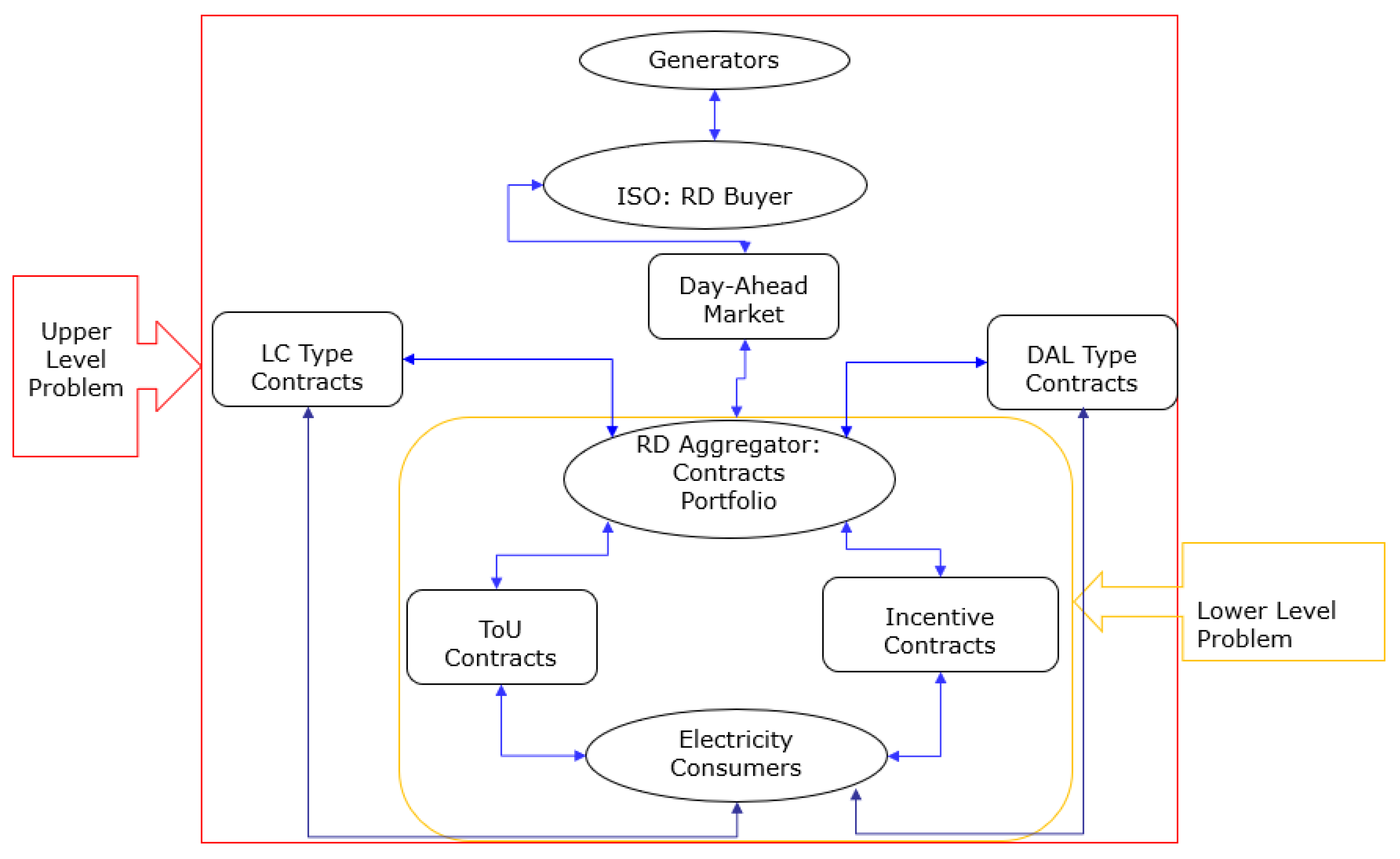
This research work addresses the situation in which a DR aggregator participates in the wholesale market and provides energy to its customers through a portfolio of bilateral contracts. At the upper level, the aggregator interacts with the Independent System Operator (ISO), through its participation in the DA market, while at the lower level the aggregator makes the dispatch of consumers’ loads, according to the preset bilateral contracts.

The participation of the DR aggregator in an open electricity market occurs in the DA instance, where it acts as a price taker, given the size of this market. In addition, it is assumed that the aggregator has an accurate forecast of the resulting price scenario it faces, based on historical market information. The authors of [25] present a comparison of the traditional algorithms used to forecast the price of electricity in the wholesale market, providing a recommendation of the approach that produces the most accurate results. This analysis is not part of our scope but is necessary for the implementation of the proposed contract composition comparison methodology.

In addition to considering the interaction of the DR aggregator upstream with the DA market, it is also necessary to take into account its downstream management through the different contracts with consumers. In this interaction, the aggregator sends economic signals of price variation or incentive that the consumers receive to solve their utility maximization problem as a function of their demand response.

The problem to be solved throughout this analysis corresponds to the definition of a methodology that allows the aggregator to establish which combination of DR contracts yields the best results concerning three evaluation criteria: greater benefit to the aggregator, greater utility for consumers, and greater reduction in electricity consumption. This methodology is illustrated through the analysis of specific cases.

This optimization problem is integrated by a higher level problem, whose objective function to maximize corresponds to the aggregator’s profit from its interaction with the electricity market and the response it receives from the consumers recruited through the bilateral contracts subscribed. Additionally, within the constraints of the optimization problem, the solution of two lower-level problems must be considered: the maximization of the utility that each consumer performs based on the electricity prices or the incentives offered, according to the type of contract subscribed and under the assumption of economic rationality behavior. Figure 1 illustrates the concatenation of these optimization problems, which correspond to the integral model that is designed.

Among the assumptions, it is important to highlight the adopted hypothesis of consumer economic rationality, which is the basis of the solution to the problem of demand response to price or incentive signals. With respect to the maximum demand considered as shiftable or reduced by consumers, we include the assumption, based on the literature, that its value can be considered as approximately 10% of the original hourly demand. Similarly, the values of consumer price elasticities are taken from those typically reported for some social groups where particular econometric analyses were performed for their definition. The methodology to conduct these econometric studies and, in general, behavioral economics and consumer demand response potential analysis is not part of the scope of our research.

3. Electricity Demand Response Aggregator Management Model

Based on optimization theory, the problem illustrated in Figure 1 corresponds to a bi-level optimization problem, given the temporality of the decisions in this problem. In the DA market, the aggregator designs the prices and, according to the characteristics of the contracts with consumers, defines its market participation. Subsequently, on the next day, users decide their level of consumption. The two levels of optimization are found in the modeling of a higher-level problem with other optimization problems as part of the constraints. These types of problems are specifically identified in the technical literature as Mathematical Problems with Equilibrium Constraints (MPEC) [26].

3.1. Upper-Level Problem

The general problem consists of maximizing the aggregator’s profit, as stated in Equation (1). This includes the purchase of energy with the wholesale market, the income it receives from the sale of energy to its consumers by considering that users are included in a DR program and the type of contract in which they are enrolled. The agreements considered are contracts for direct control type LC and type DAL, and contracts for indirect control type ToU and Reduction by Incentive (RI). This maximization is subject to constraints (2) and (3).

$$\begin{array}{cc}\hfill \underset{p^{A,DA}(t),q,v,inc}{\max }& \sum _{tϵT}(L^{DA}(t)p^{A,DA}(t)+L^{DA}(t)P^{Fix}(t)+\sum _{kϵ{\Psi }_{pi}}d(t,k)R(t)+\sum _{hϵ{\Psi }_{in}}(d(t,h)R_0(t)\hfill \\ \hfill & -(D_0(t,h)-d(t,h))\eta (t,h)A(t,h))+L_{prom}^{DA}(\sum _{zϵ{\Psi }_{lc}}(D_0(t,z))-p^{lc}(t))\hfill \\ \hfill & -B(t)p^{lc}(t)+L_{prom}^{DA}\sum _{yϵ{\Psi }_{dal}}{D}_0(t,y)+{\rho }_{min}{p}^{dal}(t))\hfill \end{array}$$

(1)

subject to

$$\begin{array}{cc}\hfill & p^{A,DA}(t)=p^{LC}(t)-\sum _{kϵ{\Psi }_{pi}}d(t,k)-\sum _{hϵ{\Psi }_{in}}d(t,h)\hfill \\ \hfill & -\sum _{yϵ{\Psi }_{dal}}{D}_0(t,y)-P^{Fix}(t)-p^{DAL}(t)\hfill \end{array}$$

(2)

$$\begin{array}{cc}\hfill & \sum _{kϵ{\Psi }_{pi}}d(t,k)+\sum _{hϵ{\Psi }_{in}}d(t,h)+\sum _{yϵ{\Psi }_{dal}}{D}_0(t,y)+P^{Fix}(t)\hfill \\ \hfill & +p^{DAL}(t)-p^{LC}(t)\ge P^{min}(t).\hfill \end{array}$$

(3)

Constraint (2) indicates the balance between the energy purchased by the aggregator and the consumption of the corresponding users. Constraint (3) imposes a minimum value of energy to be consumed.

3.1.1. Direct Control Load Curtailment Contracts (LC)

The restrictions inherent to LC-type direct control contracts correspond to their dispatch and the number of times they can be activated. The binary variables define whether they are active (value of 1) and guarantee that the number of activations of each of these does not exceed the maximum established [18].

$$\begin{array}{cc}\hfill & p^{LC}(t)=\sum _{cϵ{\Psi }_{LC}}{q}^{LC}(c,t);\forall t.\hfill \end{array}$$

(4)

$$\begin{array}{cc}\hfill & q^{LC}(c,t)\le q^{(LC,max)}(c)v^{LC}(c,t),\forall t,cϵ{\Psi }_{LC}\hfill \end{array}$$

(5)

$$\begin{array}{cc}\hfill & q^{(LC,min)}(c)v^{LC}(c,t)\le q^{LC}(c,t);\forall t,cϵ{\Psi }_{LC}\hfill \end{array}$$

(6)

$$\begin{array}{cc}\hfill & \sum _{tϵT}{v}^{LC}(c,t)\le {MN}^{LC}(c),\forall t,cϵ{\Psi }_{LC}.\hfill \end{array}$$

(7)

$$\begin{array}{cc}\hfill & v^{LC}(c,t)ϵ[0,1],\forall t,cϵ{\Psi }_{LC}.\hfill \end{array}$$

(8)

Equation (4) corresponds to the sum of the energy of each one of the LC type contracts dispatched in hour t. The value assigned to each contract corresponds to a value between the maximum and minimum load, Equations (5) and (6), defined for each one. This activation depends on the value taken by the binary variable $v^{LC}$, on which the count is performed to ensure that the maximum number of activations is not exceeded, Equation (7). Equation (8) indicates that $v^{LC}$ is a binary variable.

3.1.2. Deferrable Activation Load Contracts (DAL)

The restrictions inherent to load contracts with deferred activation correspond to their dispatch, where the binary variables define their activation (value of 1) and control that the cumulative duration of the activation of each one of them corresponds to the time window established in the binding agreement.

$$\begin{array}{cc}\hfill & p^{DAL}(t)=\sum _{cϵ{\Psi }_{DAL}}{q}^{DAL}(c)v^{DAL}(c,t),\forall t.\hfill \end{array}$$

(9)

$$\begin{array}{cc}\hfill & \sum _{tϵT}{v}^{DAL}(c,t)=TH(c),\forall cϵ{\Psi }_{DAL}.\hfill \end{array}$$

(10)

$$\begin{array}{cc}\hfill & v^{DAL}(c,t)ϵ[0,1],\forall t,cϵ{\Psi }_{DAL}.\hfill \end{array}$$

(11)

Equation (9) presents the total deferred energy at time t, given the activation of the corresponding contract, by means of the binary variable $v^{DAL}$. Equation (10) ensures that the time window in which the deferrable load of each contract must be activated is exactly met. Equation (11) indicates that $v^{DAL}$ is a binary variable.

3.2. Lower-Level Problem

As mentioned in Section 2, the lower-level problem corresponds to that faced by the consumer of the variable price program (ToU Contract), Equations (12)–(14), and the consumer of the incentive program, Equations (15)–(17). Their objective functions correspond to maximizing their utility, having energy demand as their decision variable [10]. The restriction of the maximum load level to transfer or reduce is given by the factor “l”, which indicates the estimated percentage of feasible loads to transfer or reduce according to the consumers’ habits and the characteristics of the electrical appliances. This value is considered as a maximum of 10% of the total load [27]. The estimation of this potential displacement or load curtailment capacity is beyond the scope of this paper. Ref. [28] illustrates how the Non-Intrusive Load Monitoring (NILM) concept can be used to disaggregate the demand of appliances susceptible to be deactivated in some periods or their number decreased in periods of simultaneous activation.

$$\begin{array}{cccc}\hfill & \underset{d(t,k)}{\max }\hfill & \hfill & \sum _t\sum _{kϵ{\Psi }_{pi}}(\beta (d(t,k))-d(t,k)R(t))\hfill \end{array}$$

(12)

$$\begin{array}{cccc}\hfill & \mathrm{subject}\mathrm{to}\hfill & \hfill & D_0(t,k)-d(t,k)\le l\times D_0(t,k),\forall t,kϵ{\Psi }_{pi}\hfill \end{array}$$

(13)

$$\begin{array}{cccc}\hfill & \hfill & & d(t,k)\ge 0,\forall t,kϵ{\Psi }_{pi}\hfill \end{array}$$

(14)

Equation (12) corresponds to the maximization of the consumers’ utility of the variable price or ToU contracts as a function of their energy consumption, considering their income minus the price that the users pays for the service. Equation (13) constrains the displacement or reduction in the load to the fraction “l” of the base consumption, while Equation (14) forces the non-negativity of the consumption of these users.

For the consumers recruited into the incentive-based DR program:

$$\begin{array}{cccc}\hfill & \underset{d(t,h)}{\max }\hfill & \hfill & \sum _t(\sum _{hϵ{\Psi }_{in}}(\beta (d(t,h))-\eta (h)A(t,h)(d(t,h)-D_0(t,h)))\hfill \end{array}$$

(15)

$$\begin{array}{cccc}\hfill & \mathrm{subject}\mathrm{to}\hfill & \hfill & D_0(t,h)-d(t,h)\le l\times D_0(t,h),\forall t,hϵ{\Psi }_{in}\hfill \end{array}$$

(16)

$$\begin{array}{cccc}\hfill & \hfill & & d(t,h)\ge 0,\forall t,hϵ{\Psi }_{in}\hfill \end{array}$$

(17)

Equation (15) corresponds to the maximization of the consumers’ utility of DR incentive contracts, as a function of their energy consumption, considering their income plus the incentive $A(t,h)$ they receive for each kWh they reduce concerning their base consumption, including the social weighting factor $\eta (h)$ towards the response to incentives. Equation (16) constrains the load reduction to fraction “l” of the base consumption. Equation (17) forces the non-negativity of the consumption of these users.

3.3. Model as a Mixed Linear Integer Mixed Problem

The approach of the optimization problem as a mixed integer linear problem that concatenates the upper-level problem with the lower-level problem, requires that the latter be solved locally and its solution be incorporated as a linear constraint of the upper-level optimization problem.

For the solution of the lower-level optimization problem, the concept of price elasticity is introduced as the consumer’s demand response to electricity price variation. Price elasticity is a standardized measure of how the intensity of use of a commodity changes when its price changes by 1%. Thus, price elasticity is a relative measure of consumer response [10].

Specifically, in a market such as the electricity sector, a higher price elasticity of demand generates a lower market equilibrium price. Elasticity is defined as the sensitivity of demand with respect to price:

$$E=\left(\frac{R_0}{D_0}\right)\times \left(\frac{\delta d}{\delta p}\right)$$

(18)

where $R_o$ is the original or initial price and $D_o$ is the basic consumption corresponding to the initial price.

If the net price of electricity varies for different periods, then demand reacts in one of the following forms:

• Some loads that are not susceptible to shifting from one period to another, such as lighting, for example, may only change their state from on to off or vice versa. Such loads, then, have sensitivity in only one period. In this case, this elasticity is called self-price elasticity. Its value is always negative. The self-price elasticity is defined by the Equation (19).
• Some consumption may be transferred from a peak period to an off-peak period. Such behavior is called multiple period sensitivity and is known as cross-price elasticity. Its value is always non-negative. The cross-price elasticity is defined by Equation (20).

According to the above, mathematically, the following expressions are derived:

$$\begin{array}{c}\hfill E(t,t)=\frac{▵d(t)}{▵p(t)}\le 0,\forall t.\end{array}$$

(19)

$$\begin{array}{c}\hfill E(t,j)=\frac{▵d(t)}{▵p(j)}\ge 0,\forall t,j\ne t\end{array}$$

(20)

where $▵d(t)$ corresponds to the change in demand between basic consumption $D_0(t)$ and final consumption $d(t)$, generated by the price change $▵p(t)$ between the original price $R_0(t)$ and the final price $R(t)$.

Once the concepts of self and cross-price elasticity have been defined, the solution of the lower-level problem is addressed, considering the consumers’ response, either to the price change or to the payment of an incentive, as the modification of their initial demand $D_0(t,\ast )$ to $d(t,\ast )$ , where * identifies whether the user corresponds to the DR program motivated by price change $(k)$ or by incentive $(h)$. The amount of a given incentive can be formulated as:

$$P(▵d(t))=A(t)▵d(t)$$

(21)

where $A(t)$ corresponds to the value of the incentive that the aggregator pays to the user for each unit of energy that decreases in time t with respect to its expected basic consumption for that period.

Based on the above descriptions, the objective functions of the lower-level problem (12) and (15) are optimized by applying the optimality conditions and assuming the behavioral hypothesis of consumer economic rationality. The consumer’s income function $\beta (d(t,k))$, in this case depending on his consumption, is assumed to be quadratic and the Taylor series expansion can be used for its representation. The algebraic handling of this exercise, which includes the explicit presence of the self and cross-price elasticities, allows us to arrive at the following economic model, expressed as a linear equation that leads to our complete mixed-integer linear programming model. Thus, Equations (22)–(28) correspond to the optimality conditions of the problems set out in Equations (12) and (15).

$$\begin{array}{cc}\hfill & d(t,k)=D_0(t,k)+E(t,t,k)\times \frac{D_0(t,k)}{R_0(t)}\times [R(j)-R_0(j)]+\sum _{j=1,j\ne t}^{24}E(t,j,k)\times \frac{D_0(t,k)}{R_0(j)}\hfill \\ \hfill & \times [R(j)-R_0(j)];\forall t,kϵ{\Psi }_{pi}\hfill \end{array}$$

(22)

$$\begin{array}{cccc}\hfill & \mathrm{with}\hfill & \hfill & D_0(t,k)-d(t,k)\le l\times D_0(t,k),\forall t,kϵ{\Psi }_{pi}\hfill \end{array}$$

(23)

$$\begin{array}{cccc}\hfill & \hfill & & d(t,k)\ge 0,\forall t,kϵ{\Psi }_{pi}\hfill \end{array}$$

(24)

$$\begin{array}{cc}\hfill & d(t,h)=D_0(t,h)+E(t,t,h)\times \frac{D_0(t,h)}{R_0(t)}\times \eta (h)\times A(t,h)\times inc(t);\forall t,hϵ{\Psi }_{in}\hfill \end{array}$$

(25)

$$\begin{array}{cccc}\hfill & \mathrm{with}\hfill & \hfill & D_0(t,h)-d(t,h)\le l\times D_0(t,h),\forall t,hϵ{\Psi }_{in}\hfill \end{array}$$

(26)

$$\begin{array}{cccc}\hfill & \hfill & & d(t,h)\ge 0,\forall t,hϵ{\Psi }_{in}\hfill \end{array}$$

(27)

$$\begin{array}{cccc}\hfill & \hfill & & inc(t)ϵ[0,1],\forall t.\hfill \end{array}$$

(28)

Equations (22)–(24) correspond to the response of the consumer recruited in the program motivated by price change, while Equations (25)–(28) correspond to the consumers of the program motivated by incentives.

Within the model, the optimal incentive value for the aggregator has been considered taking into account that the cost to be paid by the consumer under this contract corresponds to the average tariff of a usual day. The optimal value of the incentive is the average difference between the DA market price and the average tariff, applicable if the market price is higher than the average tariff. This incentive in the model is activated through the binary variable $inc(t)$, as indicated in Equation (25), so that this only occurs when the model considers it pertinent in its objective of maximizing the aggregator’s profit.

In Equations (22) and (25), the elasticity matrix E corresponds to a square matrix of $n\ast n$, where n corresponds to the number of periods considered in the day, in which the terms of its diagonal correspond to the coefficients of self-price elasticity. These negative coefficients on the diagonal indicate the magnitude of the reaction in its demand in period t to a price change or an incentive in period t. The coefficients outside the diagonal correspond to the coefficients of the cross-price elasticity. This means that column j of this matrix indicates how a change in price during period j affects demand during each period of the day [10].

The conformation of the elasticity matrix allows the characterization of consumers according to their behavior. When the non-zero elements in column j are above the diagonal element it means that consumers react to a high price by shifting their consumption to earlier hours. On the contrary, if the non-zero values are below the diagonal element, these consumers react by shifting their consumption to hours after hour j. Consumers who can reschedule their consumption to the hours with the lowest price, usually in the early morning and at the end of the day, are called “optimizing consumers” so that the non-zero elements are located in the first and last hours of column j. The “inflexible consumers” that have in their columns the non-zero elements in the hours around the diagonal element are those who can only partially shift their consumption to hours adjacent to their usual schedule.

If a price variation in period j induces to reorganize its production without a reduction in energy demand , the sum of the coefficients of column j is equal to zero (lossless matrix). On the other hand, if consumers reduce their total demand during the day, this summation is less than zero.

In practice, the set of all consumers is composed of a mixture of all the types described above. Therefore, the structure of the elasticity matrix and the value of its elements must be determined by analyzing the response of consumers to actual price deviations from expected values. Studies on this parameter have obtained varying values for the self-price elasticity of electricity in the range of −0.25 [29]. In [30], the author presents a methodology and the computer tools that allow its implementation in order to establish the price elasticity of different groups of consumers, according to the historical patterns of their behavior, through the consideration of time series. The analysis of these methodologies is not included in this article.

Another aspect included in the developed model, related to consumer behavior, is the consideration of a threshold at which no reaction occurs until the variation of the price or incentive has a minimum percentage value, with respect to the expected price [27]. The value of this variation parameter to obtain a reaction has been set in the model as 5% of the original price.

In Equation (25), the factor $\eta (h)$ has been included which considers the difference in the responses by consumers to a similar net effect of price variation and an incentive. According to the technical literature, the reaction of consumers in response to a price-based and an incentive-based program can be classified into three groups [10]:

• Consumers have the same behavior to an incentive and to a price variation. $\eta (h)$ = 1.
• Consumers with greater reaction to a price variation. $\eta (h)$ < 1.
• Consumers with greater reaction to an incentive. $\eta (h)$ > 1.

The calculation of this factor for a specific society and the determination of a mathematical model for $\eta (h)$ requires extensive socioeconomic research based on historical data and real-time surveys.

The complete model of the mixed-integer linear problem, therefore, corresponds to the maximization of the objective function of the upper-level problem, with the linear constraints corresponding to Equations (2)–(11), related to the upper-level problem, and Equations (22)–(28), corresponding to the solution of the lower problem:

$$\begin{array}{cc}\hfill \underset{p^{A,DA}(t),q,v,inc}{\max }& \sum _{tϵT}(L^{DA}(t)p^{A,DA}(t)+L^{DA}(t)P^{Fix}(t)+\sum _{kϵ{\Psi }_{pi}}d(t,k)R(t)+\sum _{hϵ{\Psi }_{in}}(d(t,h)R_0(t)\hfill \\ \hfill & -(D_0(t,h)-d(t,h))\eta (t,h)A(t,h))+L_{prom}^{DA}(\sum _{zϵ{\Psi }_{lc}}(D_0(t,z))-p^{lc}(t))\hfill \\ \hfill & -B(t)p^{lc}(t)+L_{prom}^{DA}\sum _{yϵ{\Psi }_{dal}}{D}_0(t,y)+{\rho }_{min}{p}^{dal}(t))\hfill \end{array}$$

(29)

Subject to:

Constraints (2) to (11).

Constraints (22) to (28).

4. Simulations and Results

4.1. Definition of Portfolio and Price Scenarios

This subsection presents the scenarios considered in the simulations with the implemented model. The scenarios and simulated cases are defined to show the impacts that the coordinated DR has on the aggregator’s profit and on the cost to be covered by the different types of consumers. Consumers are classified according to the contract subscribed, through a portfolio that includes the types of contract defined here. This analysis includes the effects of varying the participation of these contracts on the same aggregate demand.

4.1.1. Price Scenarios

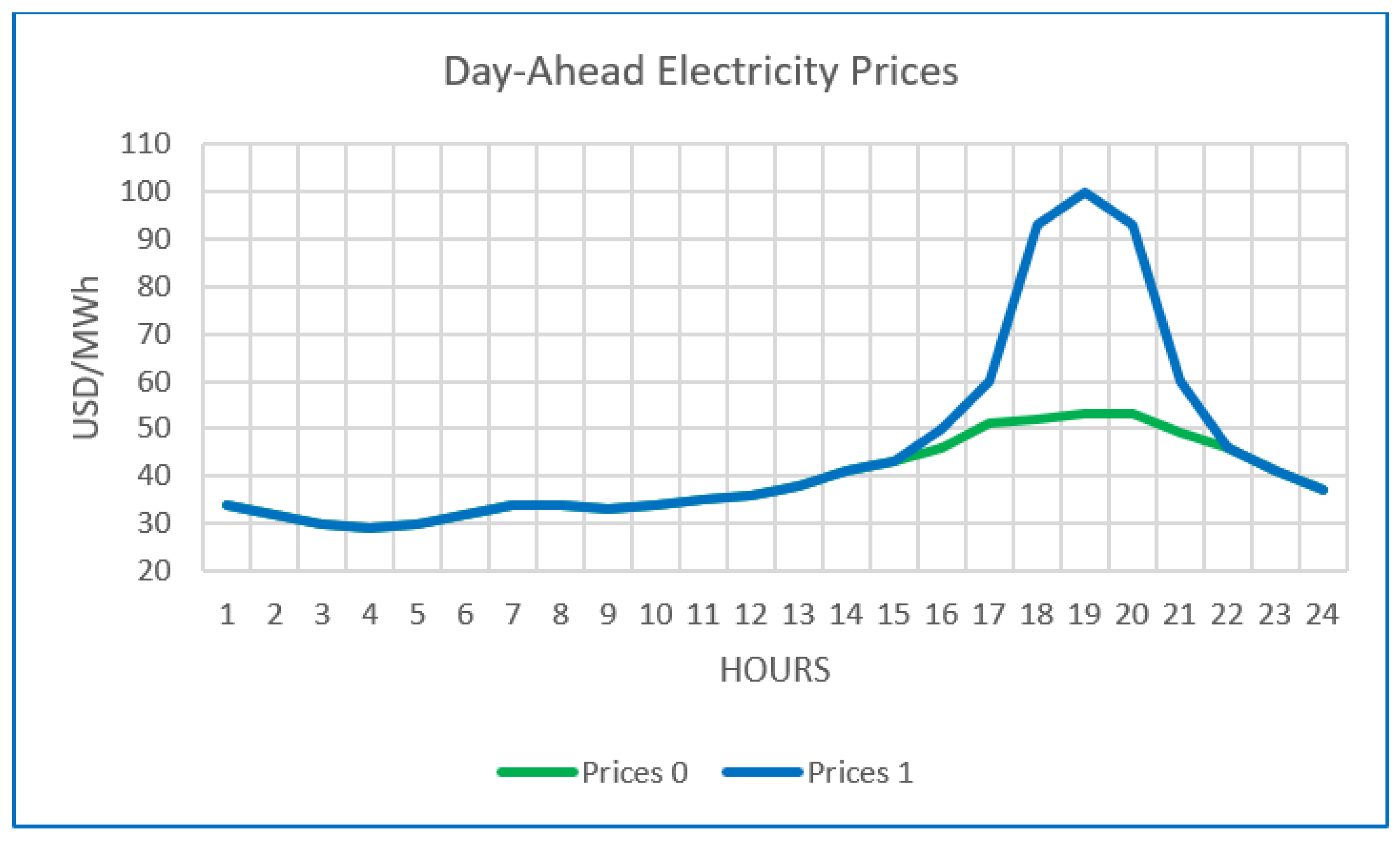
Two scenarios of hourly electricity prices in the DA market are selected for the analyses (see Figure 2), namely:

• Base Case (Prices 0): Corresponds to a typical electricity price curve of a usual day, where there is no peak price event. The information used represents a scenario of usual prices of the CAISO (California Independent System Operator) system, specifically for July 2015 [31].
• Case High Prices in Peak Hours (Prices 1): This price curve presents hourly values similar to the usual ones in off-peak hours, but its prices increase significantly in peak hours. This scenario corresponds to those days when, for example, a system with an energy matrix highly dependent on hydrology goes through a strong drought and high decrease in the levels of reservoirs. In this type of event, demand during peak price hours is usually met by dispatching generation sources dependent on high-cost liquid fuels. Figure 2 shows the curves that describe the price scenarios considered in the simulations.

4.1.2. Portfolio Scenarios

In the definition of these scenarios, the composition of the portfolio corresponds to the percentage allocation of four types of contracts, two of direct control and two of indirect control: Load Reduction Contracts (LC), Deferrable Load Activation Contracts (DAL), Reduction by Incentive Contracts (RI) and Price Variation Contracts (ToU), respectively.

In order to quantify the effects of the implementation of the DR program, the aggregate demand, prior to the implementation of the program, of the consumers coordinated by the aggregator is established as a baseline. For each hour of the day there is a defined amount of energy, assuming perfect homogeneity in the demand of each user. In this baseline, all consumers are subject to a single tariff for each kWh consumed in any of the 24 h; this tariff corresponds to the weighted average tariff of a usual day. A usual day is understood as one in which there is no punctual or sustained peak price event, concerning short-term historical information.

To capture the effect of the difference in the composition of the contract portfolio, discrete cases are analyzed, starting with an equal participation of each of the contract types; that is, each 25% of consumers participate with a different type of contract, among the four defined types. Subsequently, this composition is modified by varying the participation of each contract from 0% to 100%, while the remaining percentage of the demand is served by the other three contracts.

It is important to highlight the restriction that the maximum demand susceptible to being reduced or displaced by each type of contract is 10% of the total demand served by that type of contract for each of the hours of the day [27].

Figure 3 illustrates the total hourly demand of the users recruited by the aggregator for an average day. It is the baseline when no DR program is implemented. This curve has been assembled based on typical load profiles in the CAISO market.

4.1.3. Particular Characteristics of the Portfolio Contracts

The characteristics adopted in each type of contract are as follows:

Contract-tsype LC (LC): Consumers recruited with this type of contract receive the electric energy service in a manner that covers their demand in exchange for the payment of the average daily tariff per MWh consumed. In the events in which the aggregator activates the DR of any of the contracts of this type, consumers reduce their consumption by the amount requested by the aggregator. Each contract predefines the range of reduction that may be demanded by the aggregator and the maximum daily number of times it may be activated. In compensation, each user receives payment of a value equivalent to the average tariff for each MWh not consumed, an amount assumed as representative of the price at which the users value the energy in their utility function. In the detailed structuring of this type of contract, the value of the penalty for non-compliance with this commitment should be considered, using analyses addressed by [4], not included in the comparative analysis approached in this paper.

DAL-type contracts (DAL): In these contracts, a maximum percentage of 10% of the loads of consumers participating in these contracts can be rescheduled during a predefined time window and shifted to off-peak hours at the convenience of the aggregator. Due to this flexibility, consumers are compensated with the lowest hourly rate charge throughout the day for each MWh defined as deferrable activation; their remaining consumption is paid at the average tariff.

Reduction by incentive contracts (RI): In this type of contract, the aggregator within its model decides in which hour to generate an incentive and the value of the incentive according to the amount of demand reduction required. This value of the incentive is determined according to the consumer’s self-price elasticity, previously established, through historical analysis of the consumer’s behavior before this input and incorporated in the contract explicitly. This characterization is not developed in this research work. The consumers, in turn, receive notice of the time and value of the incentive, as well as the target load reduction. The rest of their demand is paid through the value of the average tariff.

ToU contracts (ToU): The aggregator defines three tariff levels of homogeneous duration (8 h), such that their weighted average, in base conditions, is equivalent to the average daily tariff. In this type of contract the consumers vary their consumption pattern according to their willingness. The behavior of the consumers is predicted by the aggregator, according to the self and crossed price elasticity of the users. The consumers pay for their consumption according to the tariff in force at the time of consumption.

4.2. Base Scenario or Price 0

Table 1. Results of the simulations in the base scenario.

Case	RI	ToU	LC	DAL	RD	CU	AB
1	0%	0%	0%	0%	0.00%	0.00%	0
2	100%	0%	0%	0%	0.89%	1.00%	257
3	50%	17%	17%	17%	0.54%	1.16%	159
4	25%	25%	25%	25%	0.37%	1.25%	110
5	0%	100%	0%	0%	0.58%	1.16%	39
6	17%	50%	17%	17%	0.44%	1.22%	86
7	0%	0%	100%	0%	0.00%	0.00%	0
8	17%	17%	50%	17%	0.24%	0.83%	74
9	0%	0%	0%	100%	0.00%	2.82%	146
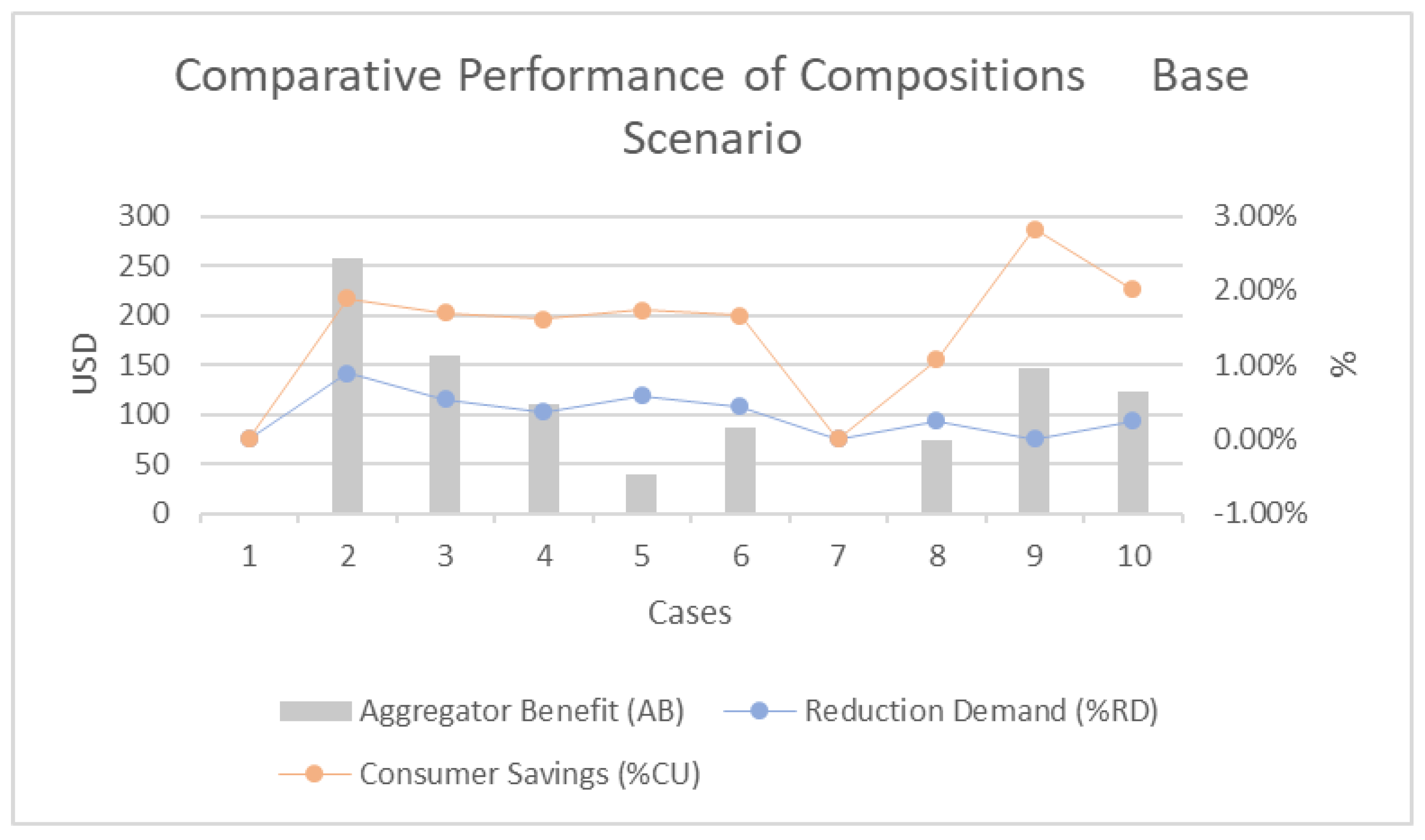
10	17%	17%	17%	50%	0.24%	1.77%	122

shows the results of the 10 cases of variation in the composition of this portfolio for the “price 0” or base case. This case corresponds to a typical day where no major peak event is generated, including that scenario where no demand response program has been implemented.The columns RI, TOU, LC and DAL present the share of each type of contract for each case, RD—demand reduction, CU—consumer utility and AB—aggregator benefit.

The comparison between the behavior of the cases is illustrated in Figure 4 and their analysis for each of the three comparison criteria used is presented in the following subsections.

4.2.1. Lower Consumer Payments

The portfolio that offers the greatest benefit to consumers is the one in which the entire portfolio corresponds to 100% of the deferred activation load contracts (DAL-type contract). This criterion is quantified as the amount that those involved save by interacting with the market and responding to the corresponding price signals. This type of demand response means, in the simulated cases, that the involved participants pay 97% of the value corresponding to the case when no DR program is present. It is worth noting that in this case demand does not suffer a net reduction.

In the base case, market prices present a deviation of ±30% concerning the average tariff, in addition to the fact that there is a correlation between typical demand and prices behavior. Therefore, there is insufficient motivation for users to significantly modify their consumption or for the aggregator to generate incentives that lead to behavioral responses. This analysis is supported by the fact that the greatest impact on consumption bills is found in contracts where up to 10% of the demand is transferred to the hour with the lowest consumption price, which is approximately 30% lower than the average daily rate.

For this variable, the next best performing compositions correspond to those where the share of DAL contracts is reduced to 50% and 25% of demand, respectively, with the rest of the demand distributed homogeneously among the other three types of contracts.

The importance of DAL-type contracts concerning the lowest price to be paid for electricity consumption is followed by the scenarios in which there is a greater participation of ToU- and RI-type contracts. The order of these two compositions is permuted if inflexible users of ToU contracts are considered.

Special interest in this simulation corresponds to the LC-type contracts, which are not activated in any of the scenarios of the base case. This behavior is explained by the fact that market prices do not offer the necessary incentive for the aggregator to dispatch this type of contract, since in none of the hours the market price is at least the double of the average tariff.

4.2.2. Higher Aggregator Profit

When analyzing the behavior of the composition of the contract portfolio for the aggregator’s profit, the case with the highest value in this variable is the one in which the RI contract corresponds to 100% of the contracts. This case is followed by the composition in which these contracts meet 50% of the demand.

This result indicates that the aggregator’s management model effectively seeks to maximize its profit by using the additional tools that this type of contract provides. This type of contract is the only one in which it has an active role in generating incentives in response to market signals and knowledge of the consumers’ elasticity.

In this case it is worth noting that after these two compositions, the best results are obtained in the cases of high participation of DAL-type contracts. These cases generate benefits to the aggregator, due to the location in the baseline of the demand classified as flexible, at times when the market price is above the average tariff. The displacement of this demand to the lowest cost hour does not totally eliminate the savings generated by its non-dispatch at those initially foreseen hours.

4.2.3. Greater Consumption Reduction

Another very important criterion in the evaluation of the performance of each composition of the aggregator’s portfolio is the net reduction in consumption in the base scenario. With respect to this variable, the composition that yields the greatest reduction is the implementation of RI contracts for 100% of the demand, followed by the implementation of ToU-type contracts for all consumers.

The above result is due to the aggregator’s action to stimulate demand reduction through strategically defined hour-to-hour incentives. On the other hand, in the composition with ToU-type contracts, the reduction is limited by the difference between the peak hour tariff and the average tariff, while another part is not reduced but shifted. DAL-type contracts do not generate demand reduction. LC-type contracts are not triggered by the relatively low differences between the average tariff and the hourly market price.

4.3. Scenario Prices 1

Table 2. Results of the simulations in the peak scenario.

Case	RI	ToU	LC	DAL	RD	CU	AB
1	0%	0%	0%	0%	0.00%	0.00%	0
2	100%	0%	0%	0%	1.75%	2.56%	2368
3	50%	17%	17%	17%	2.70%	5.78%	1372
4	25%	25%	25%	25%	3.15%	7.33%	873
5	0%	100%	0%	0%	1.13%	3.32%	76
6	17%	50%	17%	17%	2.49%	6.04%	608
7	0%	0%	100%	0%	9.96%	19.93%	1164
8	17%	17%	50%	17%	5.33%	11.36%	969
9	0%	0%	0%	100%	0.00%	4.00%	−110
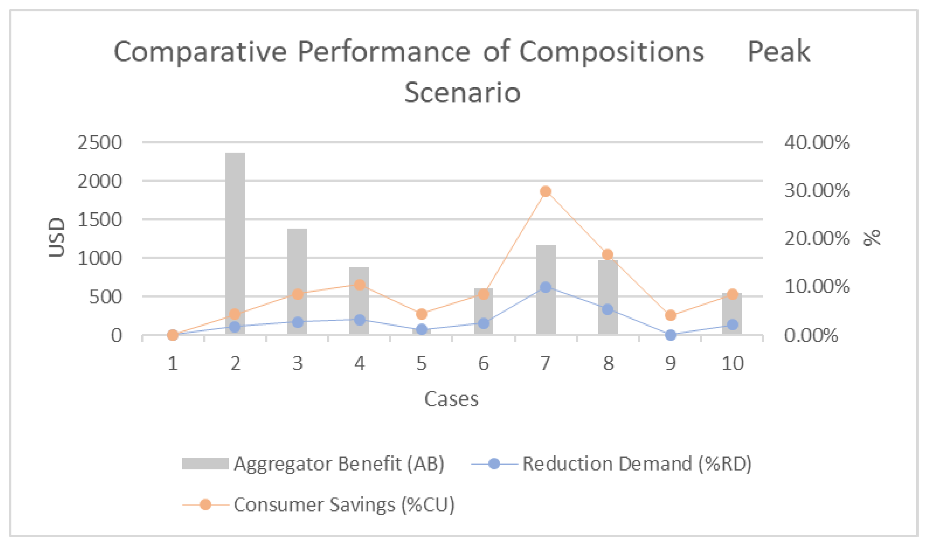
10	17%	17%	17%	50%	2.12%	6.26%	546

shows the results of the 10 cases of variation in the composition of this portfolio, including that scenario where no demand response program has been implemented, for the “price 1” or Peak case. This case presents hourly values similar to the usual ones in off-peak hours, but its value increases significantly in peak hours.

Similar to the base price scenario, Figure 5 illustrates the comparison between the behavior of the cases, characterized by different percentages of the types of DR contracts considered in this study. The analysis with respect to each of the comparison criteria used is presented in the following subsections.

4.3.1. Lower Consumer Payments

In this case, the portfolio that offers the greatest benefit to consumers is the one in which the entire portfolio corresponds to 100% of LC-type contracts. This result is followed in decreasing order by those in which its share is 50%, 25% and 17%. Among the latter, consumers obtain a lower cost when they are accompanied by a 50% share of DAL-type contracts, 50% of ToU-type contracts and 50% of RI contracts, in that order.

The above result highlights the importance of LC-type contracts in peak events where, with prices higher than double the average daily tariff, these contracts are activated generating both a significant decrease in consumption and an important benefit for the aggregator. In contrast, in the base scenario there is no activation of this type of contracts.

In the case of 100% of the LC-type contracts, users pay a value equivalent to 80% of the cost they would have to pay in a scenario with no DR program implemented. In fact, the percentage savings of all compositions in this case are higher than those calculated in the base case, showing that demand response programs have a greater impact on peak price events.

4.3.2. Higher Aggregator Profit

With respect to the aggregator’s benefit, the scenario that yields the best result in this criteria is the one in which the RI contract corresponds to 100% of the contracts, followed by the composition in which these contracts meet 50% of the demand. In this case, the LC-type contracts with 100% and 50% participation yield the highest benefit for the aggregator after those scenarios where the percentage participation of the RI contracts is dominant. As in the base case, this result indicates that the aggregator model maximizes its profit by actively generating incentives in response to market signals and knowledge of consumers’ self-price elasticity. Likewise, with the peak price levels of the simulated case, it is attractive for the model to activate LC-type contracts, achieving benefits for the aggregator to the extent that market prices are greater than twice the average tariff.

4.3.3. Greater Consumption Reduction

Finally, with respect to consumption in this case, the composition that results in the greatest reduction is the implementation of LC-type contracts for 100% of the demand, followed by those where their participation is 50%, 25% and 17%. Among the latter, a greater net reduction in demand is obtained when they are accompanied by a 50% share of RI contracts, 50% of ToU contracts and 50% of DAL contracts, in that order. Again, this result shows the benefits of LC-type Direct Control contracts in peak market events, where the massive reduction in consumption is generated in the highest price hours, normally coinciding with the highest demand hours. Likewise, after this type of contract, it is followed in effectiveness for this criteria by the RI contracts, given the action of the aggregator in stimulating the reduction in demand through incentives strategically defined.

4.4. Joint Analysis of Results in the Price Scenarios

The previous sections present the comparative results of the different cases of percentage composition of the DR contract portfolio, both for the 0 or base price scenario and for the 1 or peak price scenario.

From these analyses it can be concluded, through the ordinal qualitative assessment of the set of the three selected comparison criteria, that the composition with the best results in the base case is that which covers 100% of the demand with RI contracts. This composition is followed by that in which 50% of the demand is covered with this type of contract, distributing the rest of the demand homogeneously among the other three types of contracts.

For the case of prices 1 or peak, the best performing composition corresponds to the one in which 100% of the demand is covered by LC-type contracts. This composition is followed by the one in which 50% corresponds to these contracts and the rest is distributed among the other three types of contracts.

Finally, adding the valuations of each of the compositions of the base scenario and the peak scenario, with a 50% weighting for each scenario, it is obtained that the best composition corresponds to 50% for RI contracts, followed by the homogeneous composition among contracts of 25% for each one.

The same behavior is exhibited by increasing the weighting of the base case to 60%. From this point, the second best option corresponds to the case where 100% of the contracts are of the RI type, maintaining as the best alternative the distribution of 50% RI contracts and the rest of the demand homogeneously distributed among the other types.

If the weighting of the base scenario increases to values above 85%, the best alternative, in this particular comparative analysis, corresponds to the composition of contracts characterized by 100% of RI-type contracts.

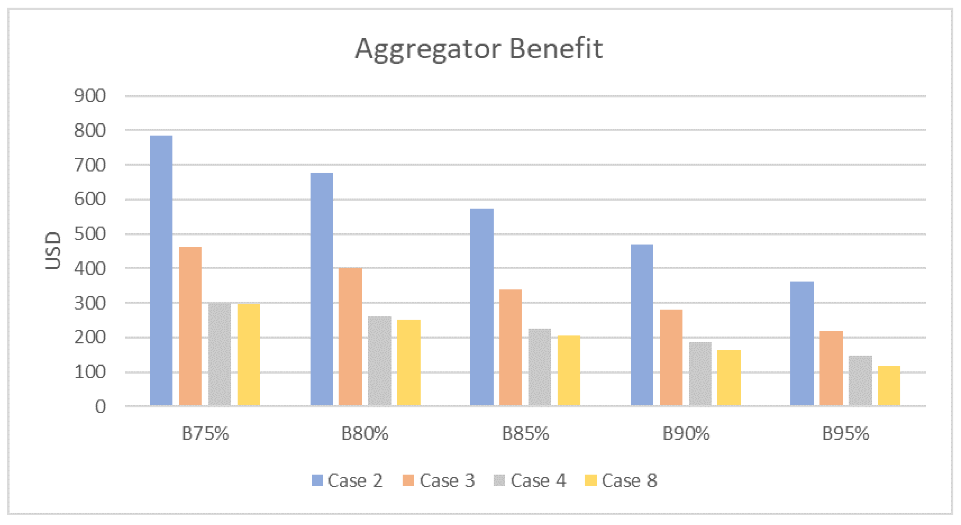
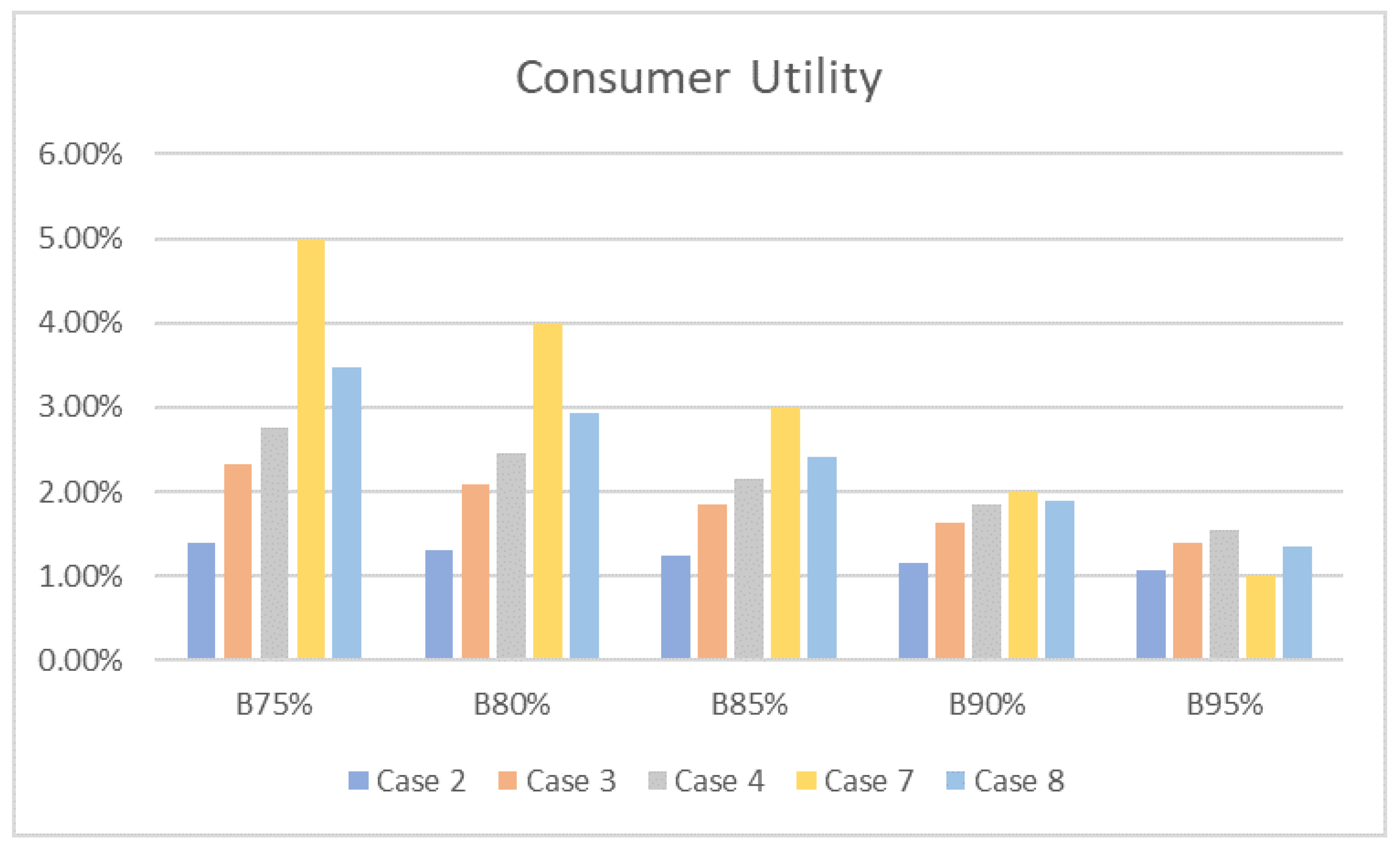
Figure 6 presents the compositions of greatest benefit to the aggregator for high weight scenarios of the base case, which correspond to the values expected in typical electricity markets. Figure 7 and Figure 8 illustrate the results of the other two criteria for these compositions, adding composition 7 in order to highlight its important contribution in demand reduction and consumer utility. The abscissa axis identifies the share of the base price scenario.

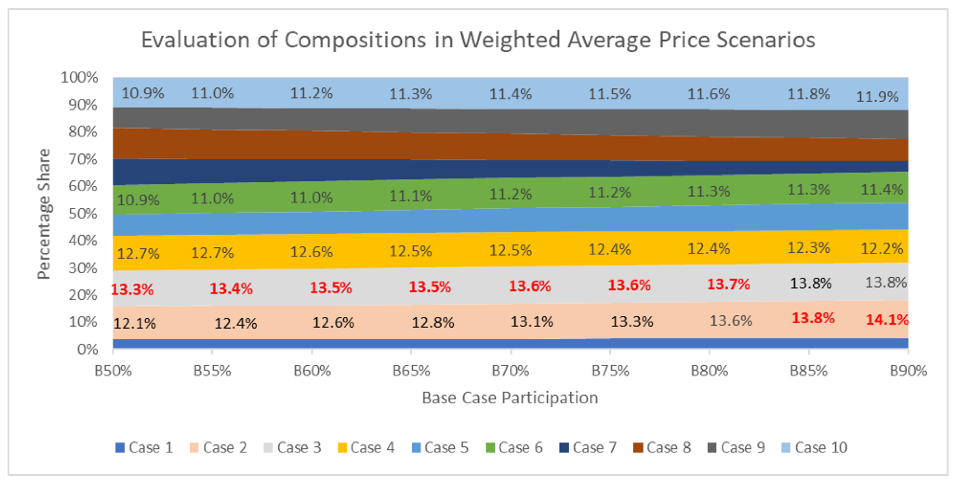
Figure 9 illustrates the comparison of the different simulated cases, considering a weighted average rating for each price scenario. In this case, an ordinal rating is used for each criterion and the same importance is assigned to the three criteria.

The analysis recommends the compositions with a high participation of RI-type contracts, according to the structure of the analysis for each type of contract in the aggregator’s portfolio.

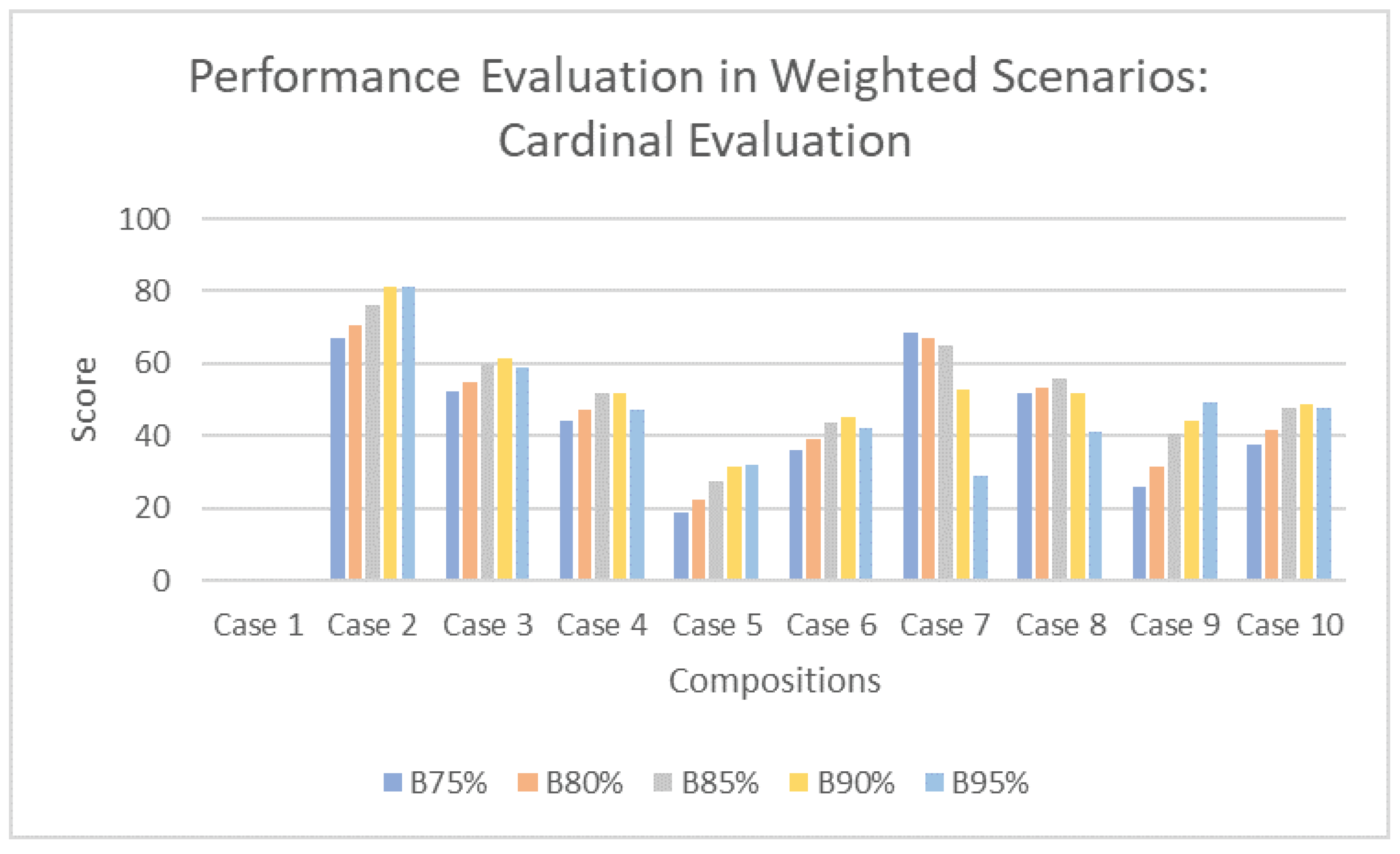
Finally, as an alternative evaluation of the consideration of the three criteria adopted in determining the best compositions of demand response contracts, Figure 10 shows the preferential order of the compositions for each weighted scenario, giving greater weight to the aggregator’s benefit criterion (50%), followed by the consumer’s utility (30%), given the importance of this criterion in guaranteeing their participation in DR programs, and the least weight to demand reduction (20%). These criteria are weighted considering their valuation from 0 to 100, with 100 being the highest value of each criterion while the other values correspond to the percentage relative to this maximum value.

This example illustrates the impact of differentiated weighting of the three criteria considered and the use of a cardinal evaluation scale. This type of evaluation better assesses the magnitude of the differences between the different compositions, beyond the score given by the place they occupy in the ranking of their results. Case 2 composition continues to be preferred in high participation levels of the base case, scenarios with higher probability of occurrence.

The weighting given to each of the criteria adopted will depend on the local and cultural context in which the aggregator intends to establish its demand response programs. Thus, for example, in a context where environmental sensitivity is a motivating factor for consumers to participate in these coordinated efforts, the demand reduction criterion should be weighted more heavily.

5. Conclusions

This article describes a methodology for comparing different combinations of DR contracts coordinated by an aggregator that recruits a significant number of consumers through the subscription of contracts . This model considers the maximization of the benefit of the aggregator and the expected behavior of the consumers. Likewise, it was shown that the proposed demand response portfolio is able to generate reductions in the load during the hours of greater demand of the system, as long as there is a timely activation of the consumers’ contracts that is adequately coordinated.

A fundamental conclusion is that the implementation of different types of contracts simultaneously allows an adequate response to different price scenarios, so that contracts that are more relevant in the face of system peak events are not so in the usual conditions of a relatively flat price curve. Applying the methodology described here, it was possible to establish the importance of characterizing the behavior of consumers to forecast their responses to the generation of specific incentives, both for the usual scenarios and for peak events. Likewise, it is shown that direct load control contracts have an important impact during periods of energy price increments, subject to the correct structuring of the commitments, the adequate determination of the price to be recognized for the demand response and the reliability of the consumption baseline.

As future lines of research, the exploration of a larger portfolio of contract types is envisioned that includes structured contracts for prosumers, involving different generation technologies, specific contracts for electric vehicles within the two possibilities: consumption only and consumption and return to the grid, as well as incentive-type contracts using the “probability of call” mechanism, described in [15]. With respect to consumer behavior, it is important to enrich the proposed methodology by incorporating econometric and behavioral economics analyses that allow for a more solid comparison when applied to a specific group of consumers. Additionally, for future analysis it is important to include the characterization of load flexibility, given the reduction in uncertainty that the aggregator will have with respect to the potential for consumer demand response.