1. Introduction
Global electricity production capacity is changing rapidly due to the phase-out of fossil power production and the decreasing cost of renewable energy production [
1]. In addition, this process is being accelerated by various national and regional energy policies and support schemes, e.g., emissions trading systems, investment subsidies and legislation on coal and nuclear phase-outs. The new capacity being installed is mostly weather-dependent solar and wind production, and such electricity generation sites are typically situated in different locations from current production capacity.
The energy transition raises the question of where this new production should be positioned within the grid. Weather conditions are one important factor in optimal positioning but there are also other considerations, such as construction costs, land usage, existing infrastructure, transmission losses and pricing of electricity [
2,
3]. The placement of power generation has previously been investigated for medium and low voltage distribution grids with smaller-scale Distributed Generation (DG) [
4,
5]. The studies found that the location of the generation sites in DG production can impact significantly the overall active power losses and system stability [
6]. So far, the research focus has been on effects at the distribution grid level due to the relatively high losses and adoption of small-scale production such as rooftop solar, fuel cells and micro combined heat and power (CHP) [
7].
Concurrently with small-scale production, a significant share of renewable electricity production capacity is in the form of utility-scale wind power and solar parks, and this capacity is thus often connected to the high voltage transmission grid [
1]. A driving factor for the use of utility-scale renewable energy production is the decreased unit costs due to economies of scale [
8]. Moreover, distribution networks may not provide the best weather and spatial conditions for larger wind and solar farms. However, compared to distributed production, centralized production increases transmission distances, thus leading to greater power losses, voltage drops and transmission congestions [
9]. To aid optimization of renewable energy systems, this article presents a method to investigate how transmission network losses and power flows are affected if power producers are incentivized to install production closer to the consumption nodes. The methods and findings can be used for network topology analysis and by policy makers for designing energy market incentives and pricing schemes.
National regulators and transmission system operators (TSO) already have tools to influence production site location. For example, production site decisions can be influenced by both energy and transmission pricing. On the energy side, the most prevalent mechanism is to divide the grid into smaller segments and price the energy separately for different parts of the grid. The division can be done on a zonal level or on a nodal level, where each consumption and production point has its unique price [
10]. These price differences incentivize power producers to locate themselves where the compensation is higher and production is more desired. On the transmission side, a common practice is to have a fixed fee per unit of energy produced and consumed. More precise network usage tariff mechanisms are also in use, for example, systems using MW-kilometers-based pricing [
11]. However, these pricing models most often only apply to the demand side and aim to steer the timing of consumption rather than the positioning of energy assets.
The question of electricity pricing is important as pricing mechanisms that do not reflect the underlying technical setup will inevitably lead to inefficient investments within the energy system [
12]. However, electricity pricing is not merely a techno-economic question, but politics are also involved. Within a single country, multiple pricing zones can be seen as a driver for discrimination between power producers and consumers in different locations [
13]. Moreover, if the pricing mechanism becomes very complex, there is a risk of non-transparency in the pricing, which can hinder long-term investment decisions. Ultimately, the choice of pricing mechanism requires balancing between these aspects.
The suitable pricing mechanism is dependent on the energy system and the corresponding network topology. Thus, it is relevant to study what type of systems benefit the most when production is steered closer to the consumption nodes. This paper presents a method that creates realistic synthetic transmission grids and analyzes the effect of distance-based value loss on such grids. The field of graph theory provides models and approaches for creating network structures such as power transmission systems [
14]. This paper uses graph theory applications to create synthetic network data and applies two different optimization models to investigate the impacts of different production positioning on power flow.
The presented method is divided into three parts. First, we create a synthetic transmission grid with randomized consumption nodes and realistic grid topologies between them. The generated network topologies are later verified with real network statistics. The second part positions power production on the network by solving a facility location problem using Mixed Integer Linear Programming (MILP) optimization and various distance-based value losses. The last part solves the AC power flow of the network and provides active power flow information about the system. The method is used to investigate a wind scenario and a solar scenario, with a similar principle than in Monte Carlo simulation, so that both scenarios are run a thousand times. Finally the impact of distance-based value losses is studied with statistical analysis.
2. Synthetic Network Topology
In constructing a synthetic transmission network, the basic principle used was to create a minimum spanning tree (MST) between the randomly generated consumption locations and to append additional network lines where it is the most cost-effective and beneficial. The approach allows the creation of topologies with several types of input characteristics, e.g., networks with high transmission distances or networks with various geographical constraints and shapes. Since the network grid represents a high voltage transmission grid, the consumption nodes serve as individual distribution grids.
A minimum spanning tree was selected as the basis of the synthetic network, as previous studies have found that in real networks, approximately 50% of power lines were also part of MST [
15]. Economically, direct power lines between nodes is the cheapest way of constructing a network but, e.g., geographical constraints can prevent their use in some cases [
16]. Direct lines were used in this paper as an approximation, since the focus of interest are the network-wide power levels rather than the individual power line bottlenecks and performance.
Of the many MST algorithms available, Prim’s method was chosen, as it reconstructs the network in an expanding fashion. Initially, only the consumption nodes are added to the network, as it is uncertain which potential production nodes will include production capacity. The network consists of number of nodes, which consist of number of consumption nodes and number of potential production sites . Matrix presents the Euclidian distance between these nodes and matrix describing the distances between nodes through the transmission lines. The transmission line topology between nodes is presented as a Boolean matrix , where a value of one indicates that a branch exists between the nodes. Lastly, the shortest paths between the nodes are stored in the matrix where paths are presented by a list of branches consisting of the shortest path. Since the distances are the same in both directions, the matrix is symmetrical along its axis and the operations are performed both row-wise and column-wise.
As Prim’s algorithm always gives the optimum solution, any of the nodes can be selected as a starting point of the network. In the algorithm, the network is expanded in each iteration with a node having the shortest distance, but now a novel step is added to update the distances and paths toward and from this new node. In each round, the new branch is selected from the subset of distances
, which have the origin node
already in the network. This group is declared as
. Out of this group, the minimum distance is selected and a corresponding branch between
and
is added into the matrix
. In the same iteration, the distances between the new node and all of the nodes existing in the grid are calculated with Equation (1). This is done by adding up the distance to the newly added branch to the distances already facing the origin node of the new branch. The path to this newly added node is created using the same principle with Equation (2). This iteration process continues until every consumption node is part of the network:
where
is the path distance matrix,
is the Euclidian distance matrix and
is the path matrix.
Since individual transmission lines can have malfunctions and overloads, redundancy is an important aspect of transmission networks. Networks often follow the N-1 principle, where no single fault can cause a system-wide outage. In this paper, the MST was combined with a method that creates shortcuts in the grid with a cost-efficiency principle. The method prefers shorter additional lines over longer ones, while at the same time creating a more circular and meshed network, hence leading to realistic power flow analysis, as presented later in
Section 6.
The shortcuts are selected by iterating over the Euclidian distances
and transmission line distances
. In each loop, the line with the shortest distance is selected from the group that met the requirement in Equation (3):
where
is a factor that tells how many times shorter the achieved shortcut should be compared to the added new line. In this research, a value of 1.25 was used for
.
Since this new line also reduces the shortest paths between the nodes of the network, the distance matrix and path matrix have to be updated. The update of the new transmission distances starts by comparing the stored distances at the nodes
and
on both ends of the new line, as presented in Equations (4) and (5). The known distances are compared and updated if a shorter distance is found:
If a new shorter transmission distance is found, the comparison continues between the node with the new shorter distances and the neighbors of the corresponding node. On the other hand, if no shortcuts are found from the direction of the new line, no comparison is performed for the other neighboring nodes. This type of breadth-first search enables information about new shorter distances to spread efficiently and ensures that comparisons are not performed on parts of the grid where they are not necessary.
3. Potential Production Sites
The next step is to generate potential production sites and allocate production at these sites. For this purpose, a variable of distance-based value loss was introduced that indicates how much the power generation is sanctioned per transmitted distance by the network operator. The unit for distance-based value loss is percentage per thousand kilometers and it compares with a capacity factor, which in turn states how much power production capacity is obtained due to weather conditions.
The potential production locations were selected randomly, after which they were connected to the closest node of the network. The maximum distance of this node was set to 20 km, so that the connecting branch would not get exceptionally long. The capacity factors varied from site to site randomly by between 35–45%. In addition, in the wind production scenario, the capacity factor increased the further up in the y-coordinate a potential production site was positioned. This presented a scenario where the network is located on a coast with windier conditions. A maximum production capacity of 1500 MW was used for all of the sites and the number of potential production sites was chosen to be equal to the number of consumption nodes to have extensive options for the site selection.
To purely research on the impact of power production positioning, it was assumed that the grid did not have any existing power production. External power sources would increase the overall power level and the marginal active power losses caused by the new production sites. However, the effect would be modest and the distance-based value loss would also consider these non-weather dependent facilities in the simulation.
4. Power Production Allocation
After the capacity factors of each potential production site and distance-based value loss was given, an optimization was performed to obtain a maximum power output of the required power production capacity. This optimization cycle was run twice for each network: first, with a distance-based value loss of zero, and the second time, with a randomized value between 0–20% per 1000 km. The first run presented a base case, where production positioning is affected only by the capacity factors, and this base case was later compared to the reference case, where distance-based value loss also has an impact. The capacity of allocated production was the same in both cases.
The model was constrained so that consumption sites
have a temporal power consumption
> 0, and potential production sites
have a capacity factor of
> 0 and power production capacity
> 0. The shortest transmission distance between the production and consumption sites is presented with
. The optimization problem is to maximize the utilized power production from the potential production sites:
where
is the production capacity,
is the capacity factor,
is the distances and
is the distance-based value loss.
In the first round of power production allocation, a base case was created where the constraint was that the power production and consumption had to match (Equation (7)) and each production site had a maximum capacity
(Equation (8)):
The solution of this optimization reveals the power production capacity of all potential production sites. In the second optimization round, where distance-based value loss was above zero, the installed production capacity was constrained to be the same as in the first optimization round, even though this does not necessarily lead to the same power production output due to the different capacity factors. Now the constraint in Equation (7) was changed to:
where
is the total consumption power and
the total installed production capacity.
The optimization problem is very similar to a facility location problem, which is a problem that was originally created to solve a factory location-based on consumer demand, production capacities and transportations costs. The problem was formulated as a Mixed Integer Linear Programming problem, which was solved using a GLPK-solver.
5. Synthetic Grid Data Topology Validation
The exact network characteristics vary between each location [
15], but the basic principle is the same everywhere: transmit the required power with adequate redundancy. It is, however, crucial to ensure that the generated synthetic network data is realistic and relevant. In this paper, the characteristics of the networks were compared to values found in prior publications [
17,
18].
The studies were done with two different scenarios, which both shared the same consumption and potential production node count and transmission line operational parameters. The differences were the geographical shape of the network and the capacity factor distribution. The chosen scenarios were a coastal wind production network and a solar production network. In the former, the capacity factors were higher on one side of the map, whereas in the latter, they were more evenly distributed. Moreover, the solar scenario had a geographically square map area (900 km × 900 km), whereas the wind scenario had a rectangular map area (600 km × 1350 km) with the shorter side representing the coast. These combinations were chosen to assess the benefits for different types of networks if production were incentivized to locate near the consumption nodes.
Table 1 presents how well the synthetic network topologies in the scenarios compare to the reference range. The reference range data is from North America, but it already comprises a notable variance between networks. In this paper, the MST was the base of the network, and additional lines were added afterwards according to the presented cost-efficiency principles. Although the share of lines on the MST was slightly greater than in the reference range, the method gave networks that otherwise corresponded well with the reference values.
6. Power Flow Calculation
Electricity does not always travel the shortest path from production source to consumption, nor does it select only one route in looped systems [
7]. Hence, power flow (PF) calculations are required to analyze power system behavior with a given network, power production and power consumption. Power flow (PF) analysis has been researched broadly and a number of established analysis methods are available [
19]. In this paper, the optimal AC power flow was calculated using the Newton–Raphson method, which has fast performance due to its quadratic convergence characteristics. A previously published Electric Power System Modeling package called Pandapower [
20] was used for the PF analysis. Since production and consumption must match exactly in power flow calculations, an additional slack bus is normally added to act either as a sink or a source in the power system. The impact of slack bus was minimized by having matching values for the total production and consumption power in the base case, but also by adding the slack bus to the node that had the shortest average distance to the rest of the nodes. The slack bus acted only as a source because the production and consumption powers were matched, but part of the power was lost due to the network losses.
The electrical characteristics were constant in each run and they are presented in
Table 2. The values are for 400 kV power lines with a triplex type aluminum cable [
21]. The values represent a strong transmission network, where the power lines have low resistances due to thick power lines and high voltage level.
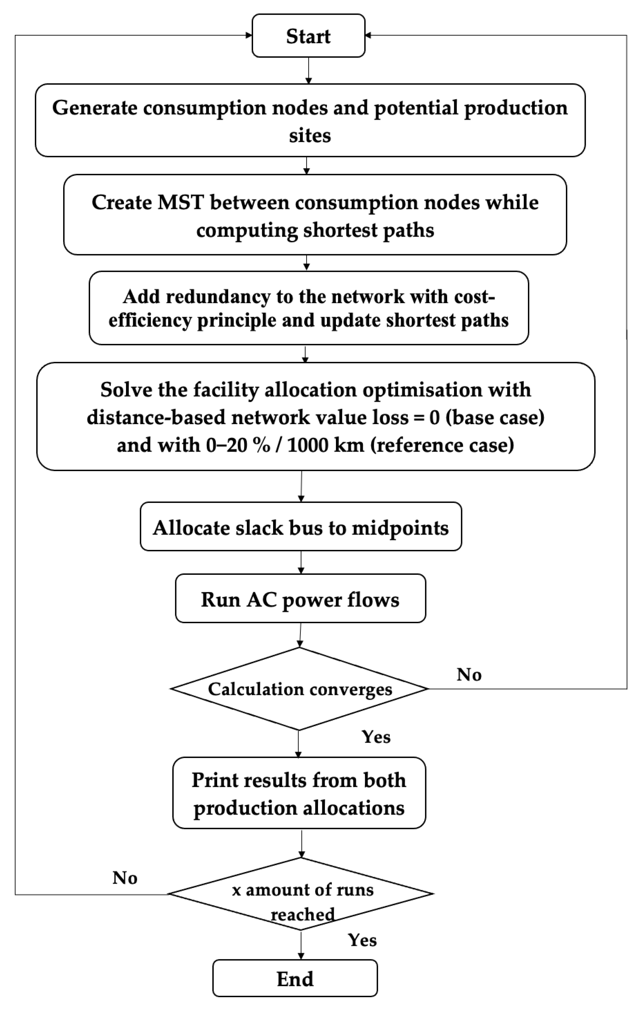
The algorithm was created with the Python programming language and the source code is available in a public repository. The algorithm flowchart, which also summarizes the computation methods used in this paper, is presented in
Figure 1. The figure shows how a network was rejected if the AC power flow analysis did not converge. Consequently, topologies with a tendency to power overloads were rejected. However, this happened only during 0.12% of the cycles.
7. Results
The presented algorithm was run with a thousand different network topologies per scenario. This approach contrasts with general transmission system analysis, where multiple scenarios and time series are analyzed against an existing single network.
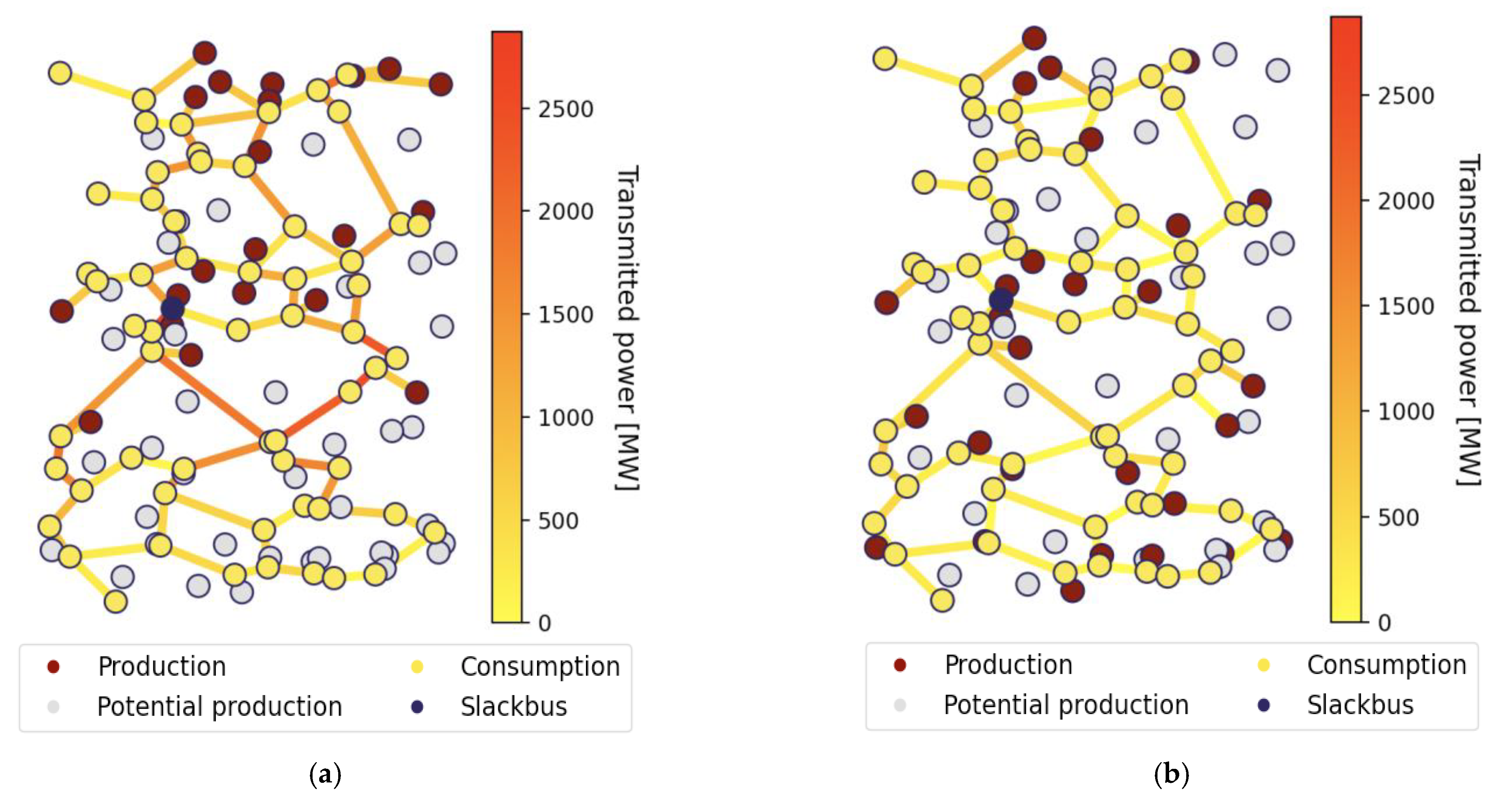
Figure 2 presents the change in production allocation when the distance-based value losses were added into the coastal wind production scenario. The geographical shape of the map area was rectangular and the windier conditions were on the top of the map. In the base case, the production was centralized on the coast area, whereas in the reference case, the optimization placed production closer to the consumption nodes. Furthermore, the production took place in a greater number of production sites. Since production was more distributed, power flow was also more evenly distributed.
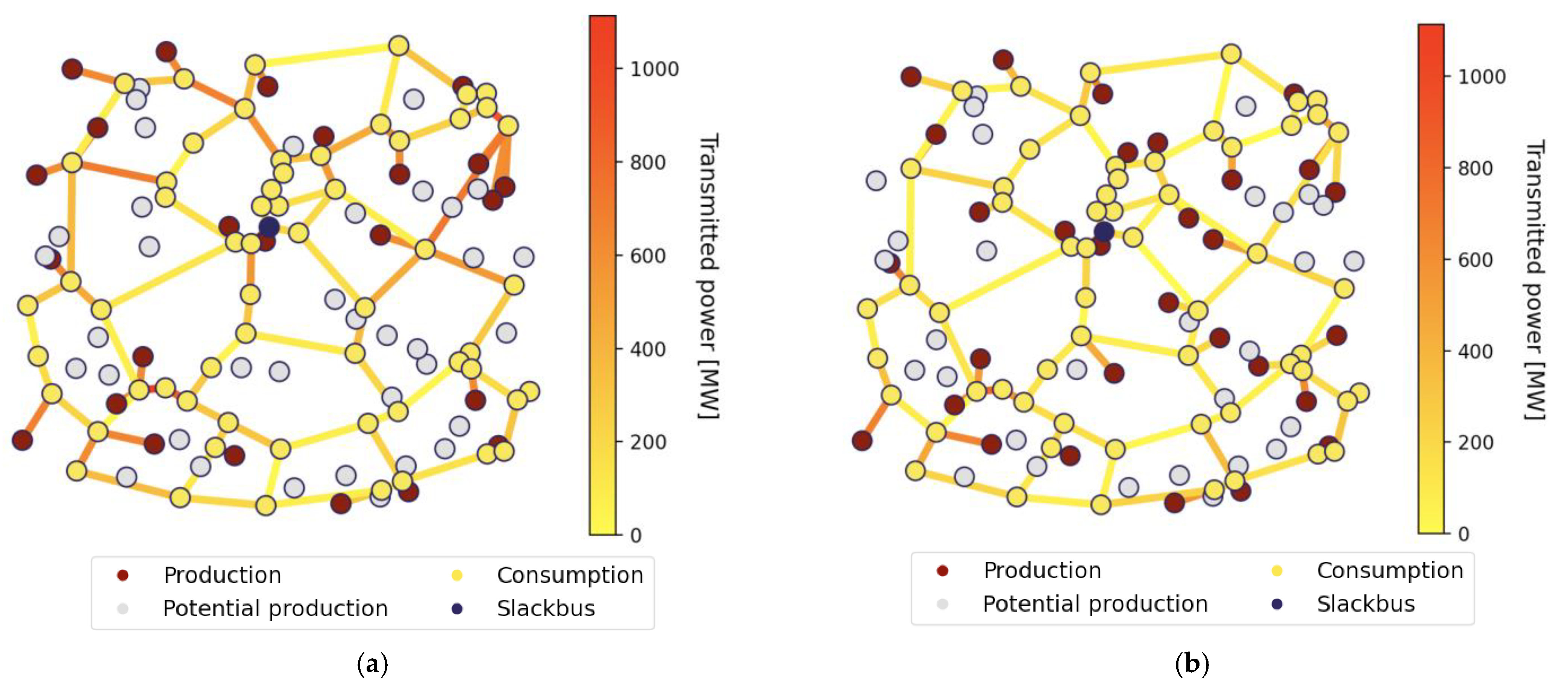
Figure 3a presents the solar scenario base case, where the capacity factors are more evenly distributed. For this reason, the distance-based value loss did not reallocate the production locations to the same degree as in the coastal wind scenario. Since the capacity factors had random variance, there were, nevertheless, variances when the facility location optimization also considered the distance-based value loss.
All the power flows were calculated with a snapshot of the system where the production powers were capacity factor times production capacity. This state represented an average scenario of production in the network. Another possibility would have been to run a longer time series against the networks and take the average of the results, but a snapshot was seen as an efficient approximation of the overall performance of the systems.
Figure 4 presents how the power flow characteristics changed in both scenarios with given distance-based value losses. The results include active power losses, production output and slack bus usage. In the figure, each dot represents a single run of the model comparing the results of the base case and the reference case. The rows in the following figures present the solar and wind scenario results, respectively.
Figure 4 presents how the increase in the distance-based value loss reduced the transmission losses but also the overall production output, as not only the best production sites were utilized. The total effect of these phenomena can be seen in how much power was required from the slack bus, which operated as an additional power source to cover the consumption needs. Running the model multiple times allowed for investigation of the relation between distance-based value loss and results. When the distance-based value loss was raised, the lost production output canceled out the benefits of decreased power losses. In the solar scenario, the benefits of including distance-based value loss on power flow changes were minor, as production was well-distributed already in the base case. In the wind scenario, the slack bus usage was reduced more efficiently, and the demand from slack bus was lowest when the distance-based value loss was approximately 4%/1000 km. This level reduced slack bus usage, on average, by 138 MW, which was 25% of the level of total active power losses and 0.7% of the overall power production.
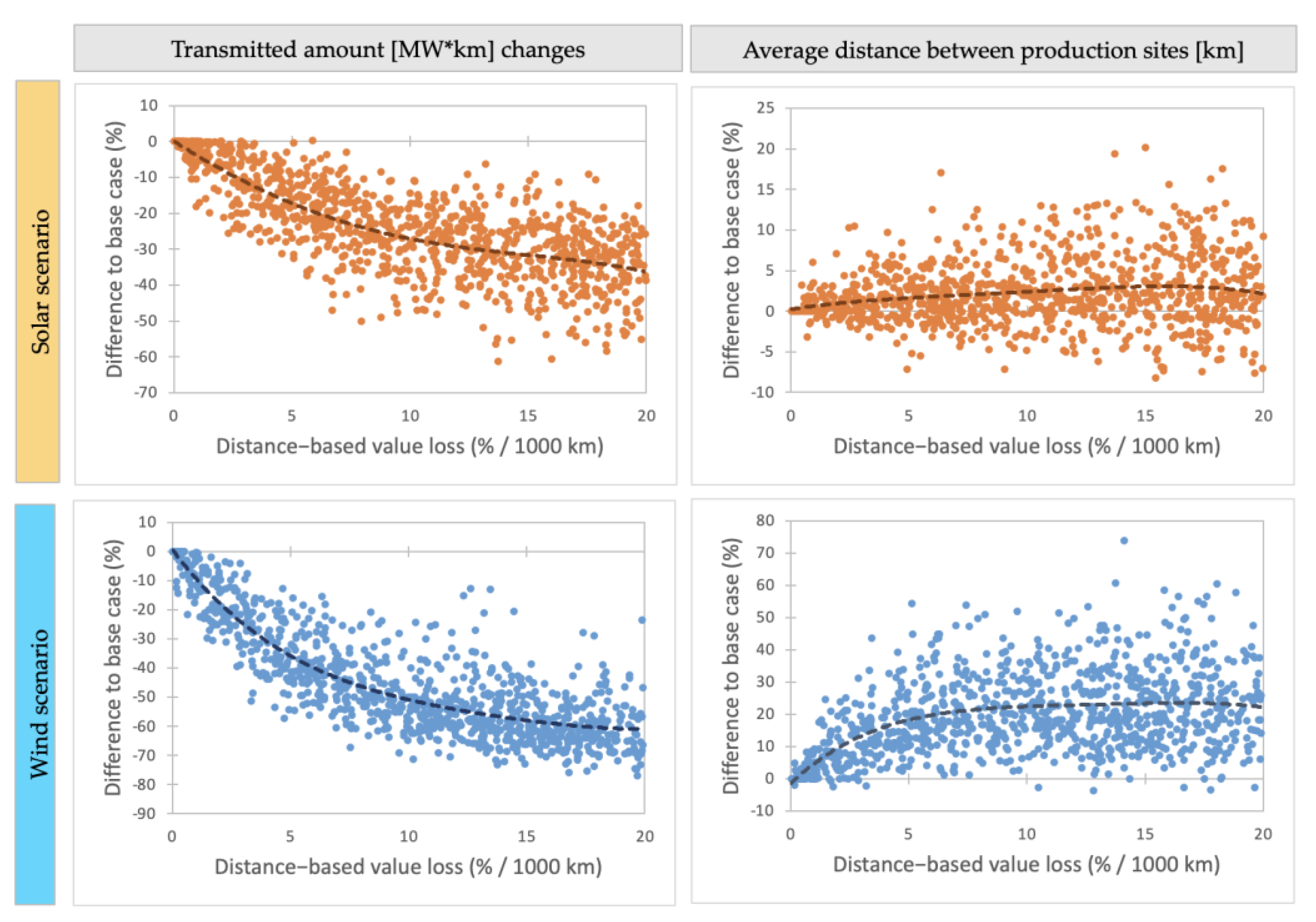
The transmission distances and power production allocation were also analyzed and illustrated in
Figure 5. The transmitted distance was a sum-product of the transmission line distances and transmitted powers per line. The value presents how much transmission capacity was utilized in the power system. The results also presented the average distance between the selected production sites, which displays how distributed the production sites were on the network.
8. Discussion
The applied method performed well in investigating the AC power flow of different network topologies. On average, it took around one second to compute a single network through the base case and the reference case using laptop with 2.6 GHz 6-Core Intel processor. The spread of the results also indicates that the generated systems had an actual variance. In addition, a comparison to prior studies revealed that the average network topology characteristics were well within the reference range.
The use of distance-based value loss reduced the overall active power losses in the investigated networks. At the same time, the achieved power output of the installed capacity decreased, as the installed capacity was not located at the sites with the best capacity factors. The total effect of these consequences was seen in usage of the slack bus that fed the missing power to the consumption sites. Analysis on multiple network topologies revealed that the use of distance-based value loss reduced the use of the slack bus, especially in the coastal wind production scenario where the benefit was greatest with a value of 4%/1000 km. The achieved benefit was then on average 0.7% of the overall power level. In the solar scenario, the benefits were smaller since the production was more distributed already in the base case.
Even though the active power losses were cut with transmission distance-aware positioning, it is worth remembering that majority of the active power losses occur in the distribution grid. A report by the Council of European Energy Regulators (CEER) surveyed European countries and found that losses in the transmission and distribution grids were 0.5–3% and 2–14%, respectively [
18]. This finding is in line with the results of this paper, with an average of 1.35% losses in the computed high voltage grids. Transmission grid is still highly relevant in the power production positioning since it is challenging to meet the consumption needs entirely with local production, and the investment costs per capacity tend to be higher in small-scale production sites.
The results indicate that the introduction of distance-based value loss into pricing or support structures was particularly effective in reducing transmitted total MW-kilometers. With a value loss of 5%/1000 km, the transmitted power distance was reduced by 40% in the wind scenario and 20% in the solar scenario. This shows that a transmission distance-based value loss may be especially useful in weaker networks with bottlenecks and relatively low capacity in the transmission lines. The long transmission distances in the base cases also underlines the importance of a strong transmission grid, so that the locations with the highest capacity factors can be efficiently utilized.
The results further revealed that a distance-based value loss caused the production to be more scattered and distributed. This feature has benefits from the perspective of system redundancy, since the power balance is not heavily dependent on certain parts of the network. Furthermore, it can enable intermittent production to have more stable power output as the production is not as heavily dependent on the weather of a single area.
The presented methodology can be further utilized to investigate, for example, optimal network topologies, the impacts of intermittent power production and the effects of various energy market designs. The model can also be extended in various ways. The investigated solar and wind scenarios were created with random and location-based capacity factors. The model assumed that the effect of varying installation costs was included in the capacity factors when allocating the production sites. The method can be extended to include installation costs and capacity factors as separate inputs. Moreover, the values do not have to be synthetic but can be based on actual observed data. In addition, the investigated transmission power systems represented solely a strong network with high voltage, a circular structure and low resistance. The networks also omitted bottlenecks that prevent power flow. The proposed method can be applied to investigate scenarios where the network is weaker due to greater resistance values, higher power level or lower redundancy. Furthermore, time series data can be used to inspect the behavior of different topologies over a longer time period.
9. Conclusions
This paper presented a method to generate synthetic transmission networks that can be used to investigate the behavior of power systems with different topologies and power production allocations. The research was done in order to examine to what extent market mechanisms should steer power production to take place near consumption sites. Selection of the right market structure is important, as a nodal or multi-zonal pricing can steer production to locations where it is most valuable. However, it can also create inequality between the price areas. This paper presented a distance-based value loss that indicated how much of the production power is sanctioned per transmitted distance. So far, the effect of production site location has mainly been investigated in the distribution grid, where the transmission losses are higher, but this paper extended research to high voltage transmission networks with a novel approach for rapidly generating a vast number of different network topologies with fixed input parameters.
The method utilized an extended minimum spanning tree algorithm and facility location optimization, and the effects were analyzed with Newton–Raphson AC power flow computation. Comparison with real power network data [
17,
18] verified that the method generated realistic transmission system topologies. Moreover, the approach was able to rapidly generate different power systems that can be used for several use cases to investigate transmission system behavior.
Analysis was done with two scenarios: a wind scenario and a solar scenario. The first scenario had the windier conditions positioned on a single side of the network, whereas the capacity factors were more evenly distributed in the solar scenario. In addition, the geographical map area was rectangular in the wind scenario and square in the solar scenario. The results indicated that a distance-based value loss of 4%/1000 km was the most efficient rate for reducing active power losses without decreasing the capacity factors of the selected production sites remarkably. However, the effect was almost nonexistent in the solar scenario. In both of the scenarios, use of distance-based value loss allocated production in a more distributed manner so that the power system is not highly reliant on the weather conditions of a single area. The distance-based value loss was also efficient at reducing the transmitted MW-kilometers, thus reducing the likelihood of transmission bottlenecks in the system. These results can be utilized in the planning of energy market structures and policies. Furthermore, the presented method can be applied in further research on transmission systems.


