Multichannel Detection of Acoustic Emissions and Localization of the Source with External and Internal Sensors for Partial Discharge Monitoring of Power Transformers

Abstract

The detection of acoustic emissions with multiple channels and different kinds of sensors (external ultrasound electronic sensors and internal optical fiber sensors) for monitoring power transformers is presented. The source localization based on the times of arrival was previously studied, comparing different strategies for solving the location equations and the most efficient strategy in terms of computational and complexity costs versus performance was selected for analyzing the error propagation. The errors of the acoustic emission source location (localization process) are evaluated from the errors of the times of arrival (detection process). A hybrid programming architecture is proposed to optimize both stages of detection and location. It is formed by a virtual instrumentation system for the acquisition, detection and noise reduction of multiple acoustic channels and an algorithms-oriented programming system for the implementation of the localization techniques (back-propagation and multiple-source separation algorithms could also be implemented in this system). The communication between both systems is performed by a packet transfer protocol that allows continuous operation (e.g., on-line monitoring) and remote operation (e.g., a local monitoring and a remote analysis and diagnosis). For the first time, delay errors are modeled and error propagation is applied with this error source and localization algorithms. The 1% mean delay error propagation gives an accuracy of 9.5 mm (dispersion) and a maximum offset of 4 mm (<1% in both cases) in the AE source localization process. This increases proportionally for more severe errors (up to 5% reported). In the case of a multi-channel internal fiber-optic detection system, the resulting location error with a delay error of 2% is negligible when selecting the most repeated calculated position. These aim at determining the PD area of activity with a precision of better than 1% (<10 mm in 110 cm).

1. Introduction

Acoustic Emission (AE) is the study and practical use of elastic waves generated by a material subjected to external stress. Strictly, acoustic refers to the pressure waves detected by ear. However, the elastic waves in solids are not limited to pressure waves, since all types of vibration modes are generated by acoustic emission sources (AES). Still, the term AE has become almost universally used for the phenomena of elastic waves generated by an internal event in a medium. In this case, acoustic refers to any elastic wave generated by an AES. Therefore, AE is the generation of an elastic wave by rapid change in the stress state of a region in the material. The change of stress must be fast enough to transmit some energy to the surrounding material. The material may be a solid, liquid, gas or plasma and the external stress can be applied mechanically, thermally, magnetically, and so forth. A large scale example may be that of an earthquake or thunder, and a small-scale example is the breakage of crystalline microstructures (metal plates, etc.).

The elastic wave generated travels throughout the material and can be detected at considerable distances from the point of origin. Thus, the characteristics of the wave (amplitude, phase, frequency, etc.) vary due to the effect of dispersion along its acoustic path. The most important information of the AE is the time of arrival (TOA) to each sensor and its amplitude. The TOA provides information on the distance of the event and the amplitude of its magnitude. The information obtained from the wave allows the calculation of the location of the AES, but the detected signals at different sensors depend on each specific path and each sensor characteristic.

Leakages, friction, impact, chemical reactions and electrical discharges (e.g., partial discharges—PD) are examples of AES. This work is based on the application of AEs from PD in power transformers [1]. Thanks to this kind of detection, the position of the AE source, and therefore the PD activity area, is detected and located [2]. There are many other applications for which the detection and location of AEs is a useful diagnosis tool, from the structural health monitoring (metals, concrete and other composite materials) [3,4], the detection of cracks in the fuselage for the aerospace industry, the detection of leaks in the chemical industry, to the analysis of insulation failures in the electrical industry.

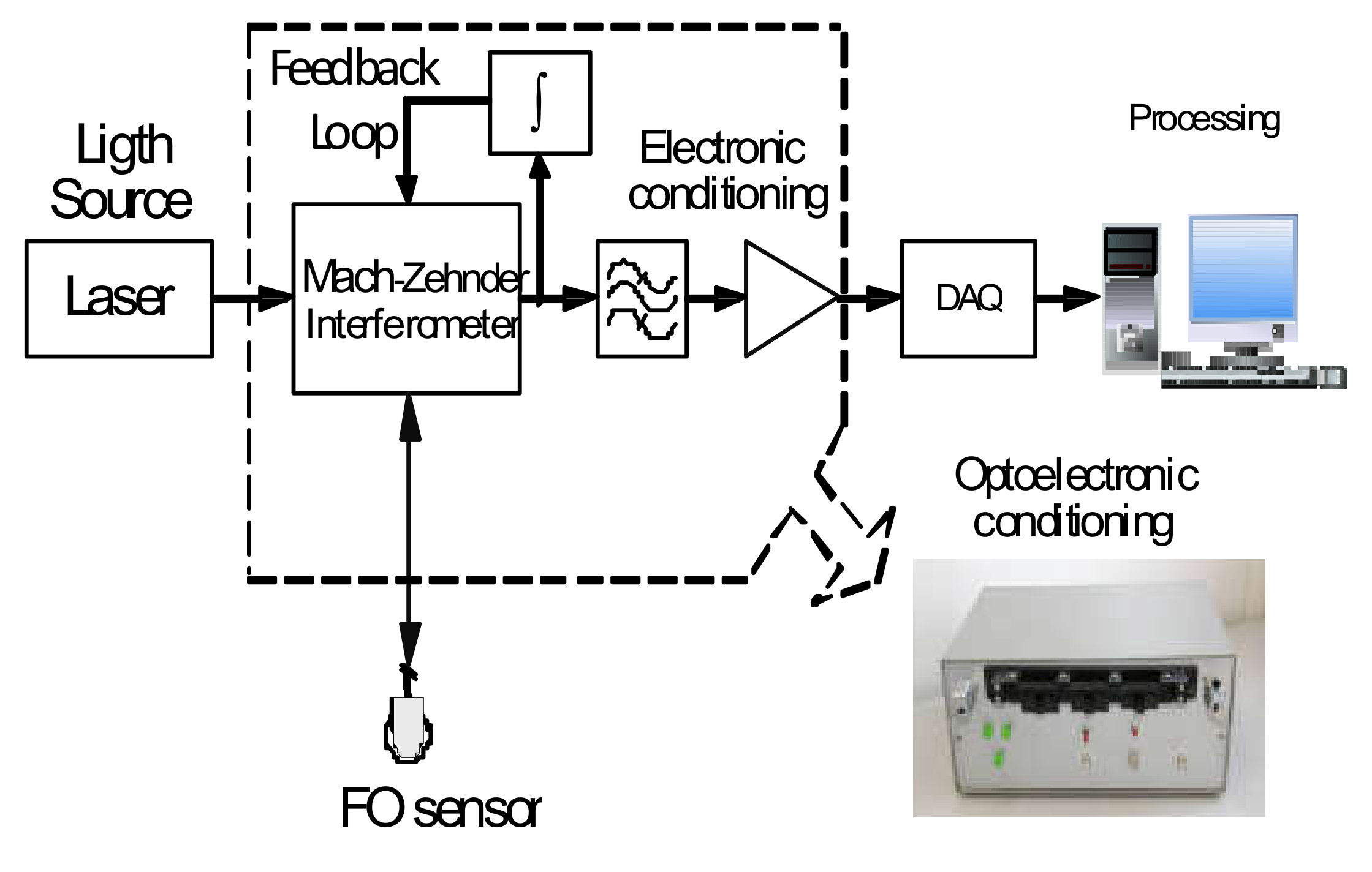
Regarding the detection of AE, piezoelectric sensors of Lead Zirconate Titanate (PZT) are typically used. In addition, other sensors that use optical fiber (OF) are being developed. In the case of detection of PD in transformers, these OF sensors are very suitable because they are embedded in the insulating medium and can detect the acoustic signal directly within the transformer tank, whereas the PZT sensors are located externally on the walls.

In the field of acoustic detection, several companies offer their equipment based on proprietary systems for specific applications that solve different aspects of the detection and processing of AE signals. The main modules are for multichannel acquisition; some of them include integrated processors and others are connected to an external PC (Personal Computer). They are usually modular devices that integrate power supplies, data acquisition cards, processors and even FPGAs (Field Programmable Gate Arrays). Some examples are AMSY-6 of Vallen Systeme [5], LAN-XI of Brüel and Kjær [6] or PXI (Peripheral Component Interconnect (PCI) eXtensions for Instrumentation) of National Instruments [7]. The instrumentation system used in this work includes the PXI. Besides having specialized modules for acquisition and signal processing, this platform has software flexibility by virtual instrumentation.

There has been an important research effort with respect to the hardware for AE monitoring, such as data acquisition, communication systems and sensor arrays [8,9,10]. The objective of an automatic AE monitoring system is the identification of the AES [11,12] and its localization. The localization is based on measurements of the TOAs of the AE signal to individual sensors of an array. Efforts are being made to implement faster and more efficient algorithms.

The hybrid programming system described in this paper is an evolution of previous systems in order to improve the performance. A previous approach included a single architecture based on LabVIEW [13]. It implemented a module of detection/conditioning and a module with an acoustic localization method based on lookup tables. It exhibited a resolution of 1 cm. However, the graphical design based on LabVIEW is inefficient with other complex algorithms that are used extensively in this kind of applications [14,15,16,17] and, therefore, a design based on Matlab was proposed for the localization stage.

As a result, the proposed hybrid programming system is as follows. A first stage is programmed in LabVIEW, which is a powerful tool for managing the acquisition with multiple channels and the on-line denoising of each channel [18,19]. The second stage is programmed in Matlab, which is a tool of numerical calculation that is specialized in data processing and representation [9,20]; thus, the localization algorithms and the presentation were programmed with this tool. The localization stage is based on the common technique of trilateration [21,22,23] and different strategies can be used [14,15,16,17]. All these methods of localization were firstly implemented in [24] with a theoretical resolution of 1 mm and they were compared experimentally. In the present paper, the hybrid programming system is described and analyzed, and the error propagation is studied (the errors of the AES location process are evaluated from the errors of the TOA detection process).

On the other hand, an OF sensor is used as an acoustic timer reference because it can be installed inside the transformer to detect PD [25]. Based on a first design of a multichannel system for the detection of acoustic emission with several OF sensors [18], in this paper, a multichannel instrumentation is demonstrated for the location of the AE source with application to PD in HV three-phase equipment. Trilateration with three acoustic sensors and a trigger reference is implemented. The experimental characterization is focused on determining the resolution and analyzing the impact of delay errors on the location accuracy.

Previous works deal with the location accuracy of a limited set of PD source positions and implement a post-processing approach for the localization algorithms. In this work, for the first time, the delay errors are modeled and error propagation is applied with this source of errors and the localization algorithms. The proposed method takes advantage of a two-stage optimization: characterization of the arrival time and location with Particle Swarm Optimization (PSO). In addition, the OF sensor provides a direct path internal acoustic reference (all acoustic location), or the OF sensors directly detect the AE (internal sensor location). Both stages communicate continuously; thus, we integrate the overall signal processing and algorithms for real on-line operation. On the other hand, this error analysis was extended to fiber-optic sensing systems.

This paper is organized as follows: the instrumentation system is described in Section 2. It was designed and implemented for the detection and location of AE based on PZT and OF sensors. The strategies for the location of the AES and their implementation are presented in Section 3. The characterization of the localization system is presented in Section 4, which includes the description of the hybrid programming system and the error propagation analysis. Finally, the conclusions are summarized in Section 5.

2. Materials and Methods

Two types of acoustic sensors have been used: OF sensors and PZT sensors. First, the general instrumentation system for the acoustic monitoring of partial discharges is presented. Second, the fiber-optic sensing probe is briefly described as a single internal sensor of acoustic emission and an all-fiber multichannel system is considered for acoustic monitoring with internal sensors.

2.1. Acoustic Monitoring Instrumentation System

Two types of acoustic sensors have been considered simultaneously: OF sensors and PZT sensors (Figure 1). OF sensors are internal and can provide a time reference for the location process. It is sensitive to the AE of 150 kHz.

The PZT ultrasonic sensors are typically used for acoustic detection. These sensors work with ultrasonic frequencies and are mounted on metal surfaces (Figure 1), for example, on the walls of a transformer tank. The use of several sensors or a sensor array allows carrying out the AES location. The model of the PZT sensor is R15I-AST (Physical Acoustics-MISTRAS Group, Princeton Jct., NJ, USA), with the following characteristics: operating range 80–200 kHz, resonant at 150 kHz, low noise integrated preamplifier of 40 dB. The sensitivity of these sensors is about 1 V/Pa. Because the sensor R15I has integrated electronics but it has no separate ports for power and output, a Bias-T circuit is necessary.

An industrial PXI has been used in order to integrate into the same system different types of sensors (PZT, OF, etc.) and signal processing units. The PXI system (National Instruments) is a PC-based open platform for test, measurement and control. It includes a data acquisition module (NI PXI-5105) with eight channels of simultaneous acquisition of 12-bit resolution, 60 MS/s acquisition rate in real time, up to 60 MHz bandwidth and 128 MB onboard memory. The graphical programming tool used is LabVIEW.

Figure 2 shows the components of the overall system: a PXI based multichannel acquisition and denoising system, an OF sensor conditioning system and a multichannel PZT sensors conditioning system.

After comparing different techniques of denoising, a combination of wavelet techniques and digital filtering was selected [1,12]. They can be used alone or together depending on the application.

2.2. Fiber-Optic Sensing Probe and Multichannel Fiber-Optic System

A single OF sensor is in Figure 3. The output of the sensor is an optical phase. Its main characteristics are as follows: frequency range of 50–200 kHz electronically filtered, resolution of 1 Pa with a phase detector of 1 mrad, and directivity of ±30° [25]. This sensor withstands severe harsh electromagnetic conditions and the temperature range inside transformers (hot spot of 110 °C is considered). Acrylate coated optical fibers withstand long-term temperatures of 135 °C and short-term temperatures of up to 200 °C. The optoelectronic conditioning scheme for the OF sensor is presented in Figure 4. It is an optical interferometer set-up with stabilization that mainly compensates the temperature drift on the sensor [25]. The resultant sensitivity is equivalent to the R15I-AST sensitivity (1 V/Pa). This implementation is used for a single internal sensor that gives an acoustically measured time reference for the localization in the system of Figure 1.

Several sensors can be implemented to locate the AE source for all-fiber acoustic detection of PD [15]. Instead of implementing four detection interferometers using the detection approach of Figure 4, we developed a four-channel opto-electronic conditioning system that is presented in Figure 5. It is a heterodyne optical interferometer set-up [10]. The optical phase of each single sensor is mapped onto a carrier signal of 40 MHz with an acousto-optic modulator. Each channel is mixed with a clock reference and filtered to obtain an electrical carrier of 4.8 MHz that contains the phase information and is acquired with the same DAQ of Section 2.1 (Figure 2). Finally, a digital I/Q phase detector is implemented for each channel in LabVIEW, which provides parallel processing.

3. Location Based on Acoustic Emission

Localized failures in the insulation system produce ultrasonic AE. The failures behave as AE sources, which can be located by means of the multichannel detection system and the use of location techniques. The location of faults provides useful information for the condition assessment, especially in a large apparatus such as power transformers [1,2].

3.1. Location by Time Diference of Arrival with OF and PZT Sensors

The common technique for 3-D spatial location of AE is the trilateration. This technique determines the position of the AES measuring the TOAs [21,22,23].

The model is a 3-D space with k + 1 acoustic sensors at specific positions (an internal OF sensor and k external PZT sensors in the surrounding of the AES). The resulting times of arrival are T from the AES to the OF sensor and T_k from the AES to the PZT_k sensor. In this case, the reference is the OF sensor (Figure 1).

There are several approaches to trilateration but, due to an all-acoustic instrumental scheme being employed in this work, the time-differences approach (time difference of arrival—TDOA) has been chosen (Figure 6).

In this case, the acoustic wave reaches the nearest sensor first (straight propagation is assumed) and it triggers the process of recording the signals from all sensors simultaneously. Four time-differences (τ_0i) are obtained from five sensors and the reference is from the sensor closest to the AES (T). Figure 6 illustrates these time differences of the acoustic signals with an unknown timing reference.

The system of nonlinear equations of a 3-D location with a time-differences approach is as follows:

$${\left(x-x_{\mathit{Sref}}\right)}^2+{\left(y-y_{\mathit{Sref}}\right)}^2+{\left(z-z_{\mathit{Sref}}\right)}^2={\left(v_s·T\right)}^2$$

(1)

$${\left(x-x_{\mathit{PZTk}}\right)}^2+{\left(y-y_{\mathit{PZTk}}\right)}^2+{\left(z-z_{\mathit{PZTk}}\right)}^2={\left(v_s·\left(T+{\tau }_{0k}\right)\right)}^2,k=1\dots N,$$

(2)

where v_s is the speed of sound in the medium, x_OF, y_OF, z_OF are the coordinates of the reference sensor and x_PZTk, y_PZTk, z_PZTk are the coordinates of the kth PZT sensor. The minimum number of sensors is 5 (N ≥ 5). The position is determined by obtaining x, y, z, T.

In [24], different methods of localization with a resolution of 1 mm were implemented and compared experimentally. In these solution strategies, except for the Particle Swarm Optimization (PSO) method [15,16,17], the equations system should be adapted to the matrix structure A*X = B. This is obtained in Equation (3) by subtracting Equation (1) from Equation (2) for k = 1 to N:

$$\begin{array}{ll}2\left(x_{Sk}-x_{Sref}\right)x& +2\left(y_{Sk}-y_{Sref}\right)y+2\left(z_{Sk}-z_{Sref}\right)z+2v_s{}^2{\tau }_{0k}T\\ & =\left(x_{Sk}{}^2-x_{Sref}{}^2\right)+\left(y_{Sk}{}^2-y_{Sref}{}^2\right)+\left(z_{Sk}{}^2-z_{Sref}{}^2\right)\\ & -v_s{}^2{\tau }_{0k}{}^2, k=1\dots N\end{array}$$

(3)

$$\begin{gathered} A=\left(\begin{array}{c}2\left(x_{S1}-x_{Sref}\right)\\ \cdots \\ 2\left(x_{SN}-x_{Sref}\right)\end{array}\begin{array}{c}2\left(y_{S1}-y_{Sref}\right)\\ \cdots \\ 2\left(y_{SN}-y_{Sref}\right)\end{array}\begin{array}{c}2\left(z_{S1}-z_{Sref}\right)\\ \cdots \\ 2\left(z_{SN}-z_{Sref}\right)\end{array}\begin{array}{c}2v_s^2{\tau }_{01}\\ \cdots \\ 2v_s^2{\tau }_{0N}\end{array}\right)\hspace{1em}X=\left(\begin{array}{c}x\\ y\\ z\\ T\end{array}\right) \\ B=\left(\begin{array}{c}\left(x_{S1}^2-x_{Sref}^2\right)+\left(y_{S1}{}^2-y_{Sref}^2\right)+\left(z_{S1}^2-z_{Sref}^2\right)-v_s^2{\tau }_{01}^2\\ \cdots \\ \left(x_{SN}^2-x_{Sref}^2\right)+\left(y_{SN}^2-y_{Sref}^2\right)+\left(z_{SN}^2-z_{Sref}^2\right)-v_s^2{\tau }_{0N}^2\end{array}\right) \end{gathered}$$

Table 1. Location solution strategies.

Type of Method	Method	Equations	N° of Sensors Used	References
Direct	“Solve” (Matlab)	-	5	-
	Least Squares (LS)	$X={\left(A^{T}A\right)}^{-1}{A}^{T}B$	5	-
	Least Norm (LN)	$X=A^T{\left(A{A}^T\right)}^{-1}B$	5	-
	Cramer	$A=\left[A_x A_y A_z A_T\right] , \left|A\right|\ne 0$ $x=\frac{\left|B A_y A_z A_T\right|}{\left|A\right|} , y=\frac{\left| A_x B A_z A_T\right|}{\left|A\right|} ,$ $z=\frac{\left| A_x A_y B A_T\right|}{\left|A\right|} , T=\frac{\left| A_x A_y A_z B\right|}{\left|A\right|}$	5	-
Indirect	Non-Iterative (INI)	-	4	[14]
	Particle Swarm Optimization (PSO)	Fitness function: $f\left(p\right)={\displaystyle \sum _{j=1}^n}{\displaystyle \sum _{i=1}^m}\left|\left[{\left(p{x}_j-x_i\right)}^2+{\left(p{y}_j-y_i\right)}^2+{\left(p{z}_j-z_i\right)}^2-v_s^2{\left(p{T}_j-{\tau }_i\right)}^2\right]\right|$ Refinement equations: $v_j\left(t+1\right)=w_k·v_j\left(t\right)+c_1{R}_1\left[p_j^{best}\left(t\right)-p_j\left(t\right)\right]+c_2{R}_2\left[g^{best}\left(t\right)-p_j\left(t\right)\right]$ $p_j\left(t+1\right)=p_j\left(t\right)+\mathsf{{\rm Y}}·v_j\left(t+1\right)$ Inertia weight: $w_k=w_{max}-\frac{w_{max}-w_{min}}{N}k$ Constriction coefficient: $\mathsf{{\rm Y}}=\frac{2}{\left|2-\gamma -\sqrt{{\gamma }^2-4\gamma }\right|} , \gamma =c_1+c_2 and \gamma >4$	5	[15,16,17]

summarizes the location solution strategies. The INI and PSO methods provided the best results (the figure of merit was precision over runtime).

The PSO algorithm has been demonstrated to be useful for different cases of the acoustic detection of PD in laboratory experiments: with OF sensors [15], PZT external sensors [16] and also with UHF sensors [17]. We verified the performance of the PSO algorithm on a system with an internal OF sensor and six external PZT sensors and compared the overall strategies of Table 1 [24]. Based on these results, the PSO strategy is more efficient in terms of computational, complexity costs and performance in laboratory conditions of measurement.

With PSO we do not assume any hypothesis before locating the source through optimization, so there is a risk that the solution found is not optimal. Reported location errors were <20 mm in a 100 cm × 120 cm × 80 cm tank [16] and <7 mm dispersion error, 20 mm offset error in a 90 cm × 55 cm × 37 cm tank [24]. More recent results include a detailed physical model of the structure inside the transformer [26] but are similar to those in [16]. In this case, PSO is applied to search the path of the acoustic signal (PSO Route Search).

3.2. Location by Time of Arrival with OF Internal Sensors

Location of the AE source is based on the measurement of the TOA of the AE signal at the sensors. The TOA and the velocity of the AE in the propagation media (transformer oil in the real application) are used in order to obtain the distance from the AE source to each internal OF sensor. Figure 7 shows an example of how the location of failures can be found using TOA-based trilateration.

In a practical application, the acoustic detection of PD is performed at frequencies around 150 kHz. Therefore, we can test the system by generating acoustic bursts of 150 kHz inside a tank and by detecting them simultaneously with three OF sensors immersed in the tank. The typical signals detected in the test are shown in Figure 8. The TOA can be obtained via software and these can be used in order to obtain the position location of the AE source.

Detection optical interferometer of four channels was presented in Figure 5. Each carrier signal of 40 MHz and the down-converted electrical carrier of 4.8 MHz contain the information of the optical phase of the correspondent OF sensor. Three channels of the DAQ digitize the 4.8 MHz carrier signals of three sensors and detect the optical phase with three I/Q demodulators in parallel. The TOA to each sensor is obtained with a zero time reference (trigger). Figure 9 illustrates the signal flow: first, the acquisition of the carrier signals; second, the phase detection; third, the determination of the TOAs; and finally, the location.

At the output of the I/Q demodulator, signals, such as those previously shown in Figure 8, are obtained. These signals are processed by a pulse detector that finds the time instance, where the AE is at each channel and calculates the time difference between a trigger signal and the AE found. In the practical application, the trigger signal can be, for example, a signal from an electrical monitoring sensor, forming an acoustic location system with an electrical trigger [1]. Finally, once the TOAs are obtained, these are used in the location block, which finds the position location of the AE source using a trilateration algorithm. If we use four fiber-optic sensing channels, an all-acoustic localization system can be implemented; therefore, the location algorithms based on TDOA and a hybrid processing system can also be applied to the detection with internal sensors (Section 3.1).

4. Results

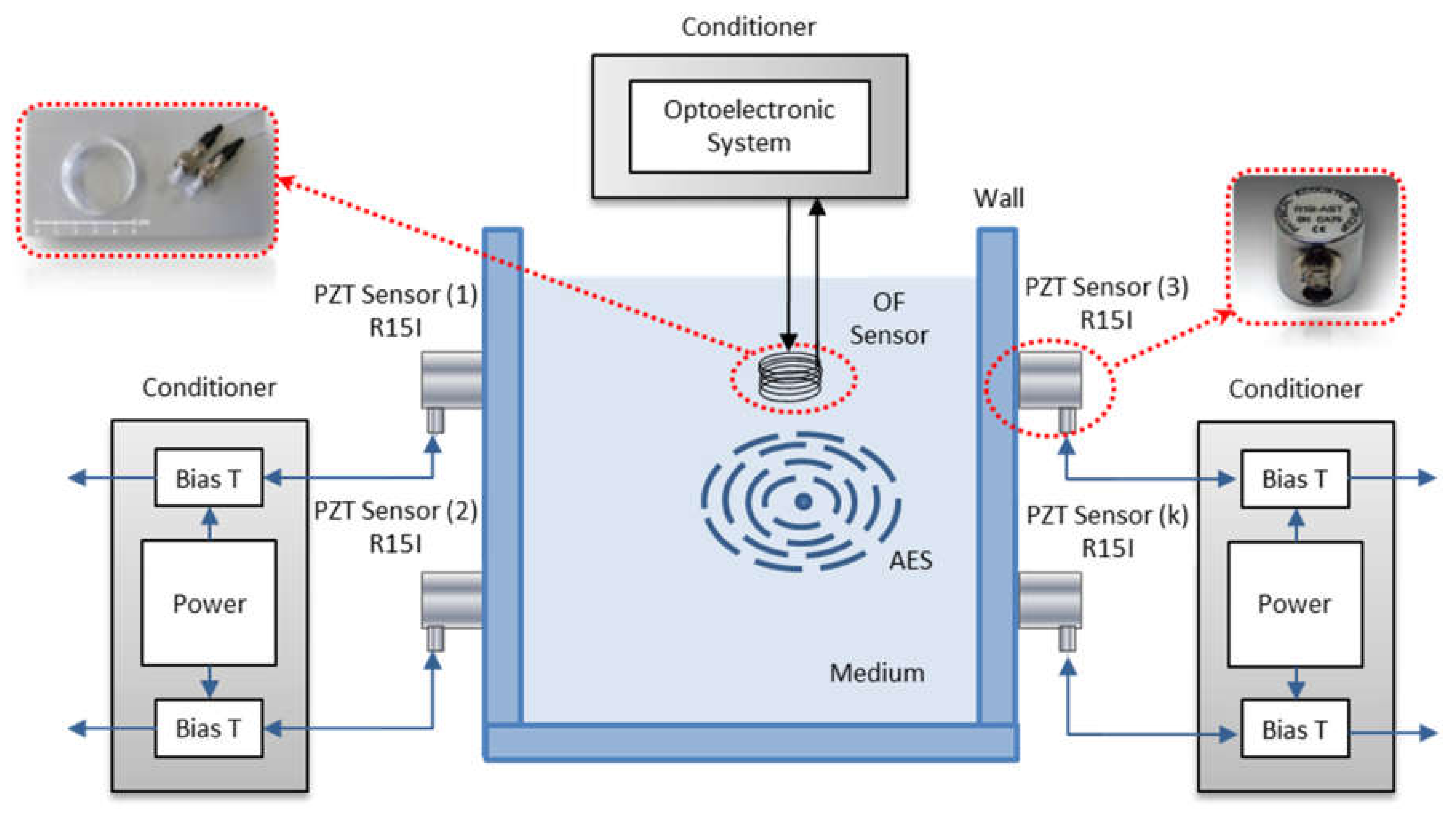
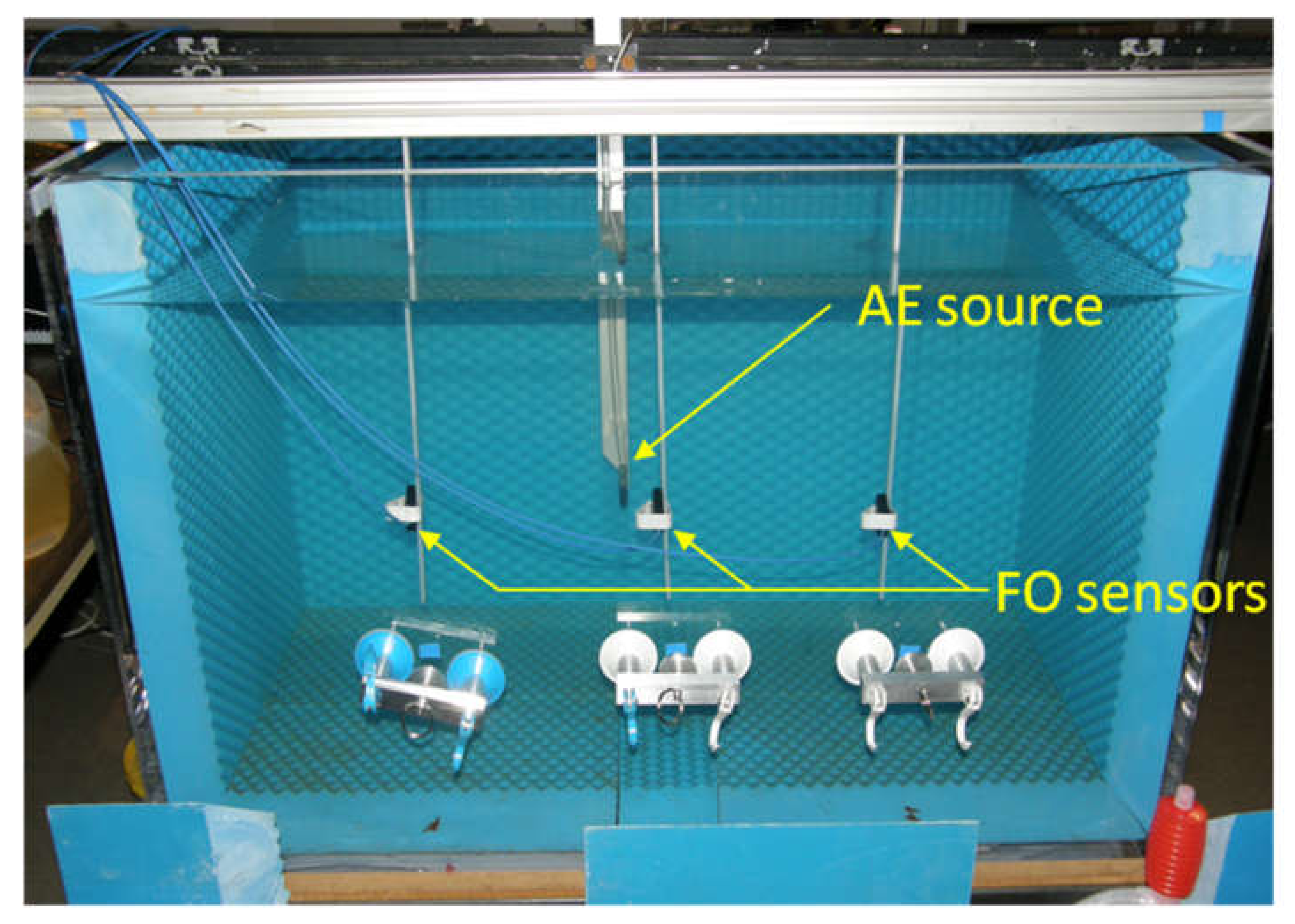
An experimental platform for acoustic emission testing was used to characterize the two systems: the hybrid processing system for AE multichannel detection and AES localization and the multichannel fiber-optic system for AE internal detection and AES localization. The experimental platform consists mainly of a container of a cubic shape and the following effective dimensions: 900 mm × 550 mm × 370 mm (Figure 10). The walls of the container are made of polymethylmethacrylate (PMMA), and the tank is filled with water. The acoustic source is a hydrophone (Brüel and Kjaër 8103). A wave generator applied to a PZT ultrasonic transducer emulates the signals from partial discharges.

4.1. Hybrid Processing System

Six PZT ultrasonic sensors have been used on the surface of a wall (R15I/AST-Physical Acoustics-MISTRAS Group, Princeton Jct., NJ, USA). In addition, an OF sensor has been used within the tank. According to the example of application, the placement of the PZT sensors follows the typical pattern of the three-phase transformers, with two sensors per phase. This platform includes only one OF sensor because of the difficulty of introducing more sensors inside the transformer tank.

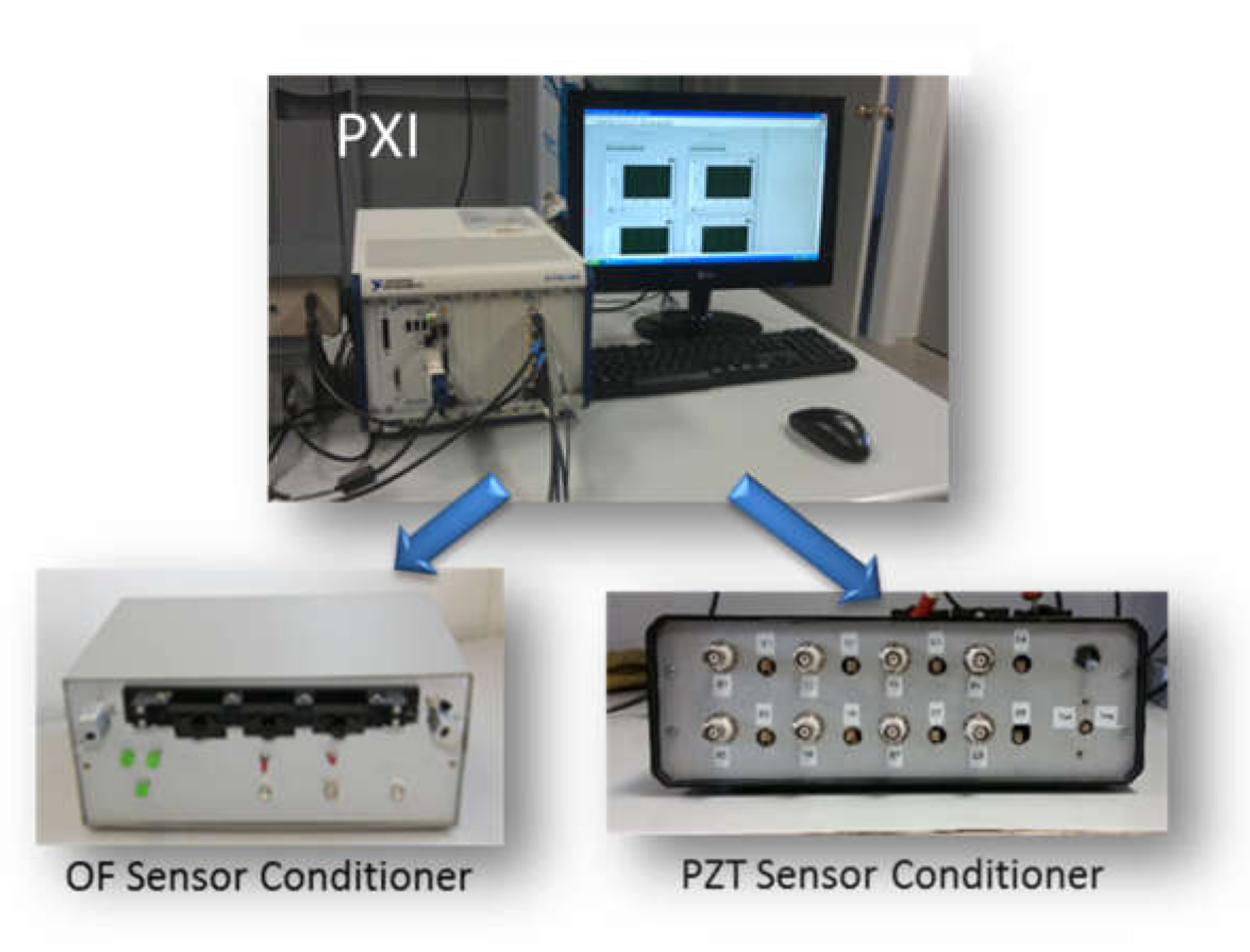
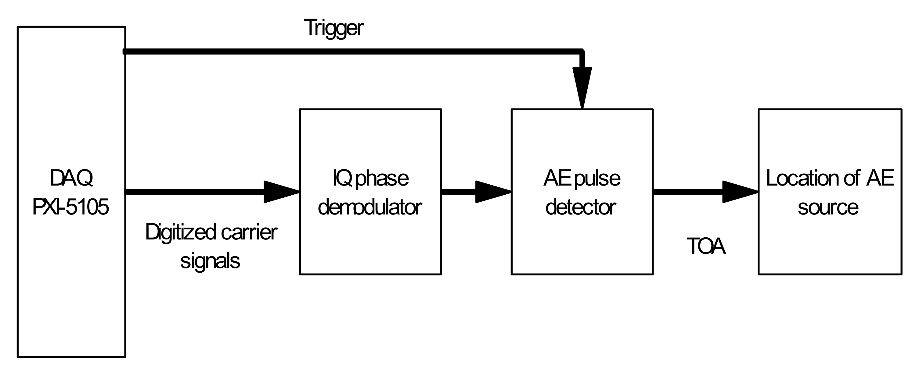
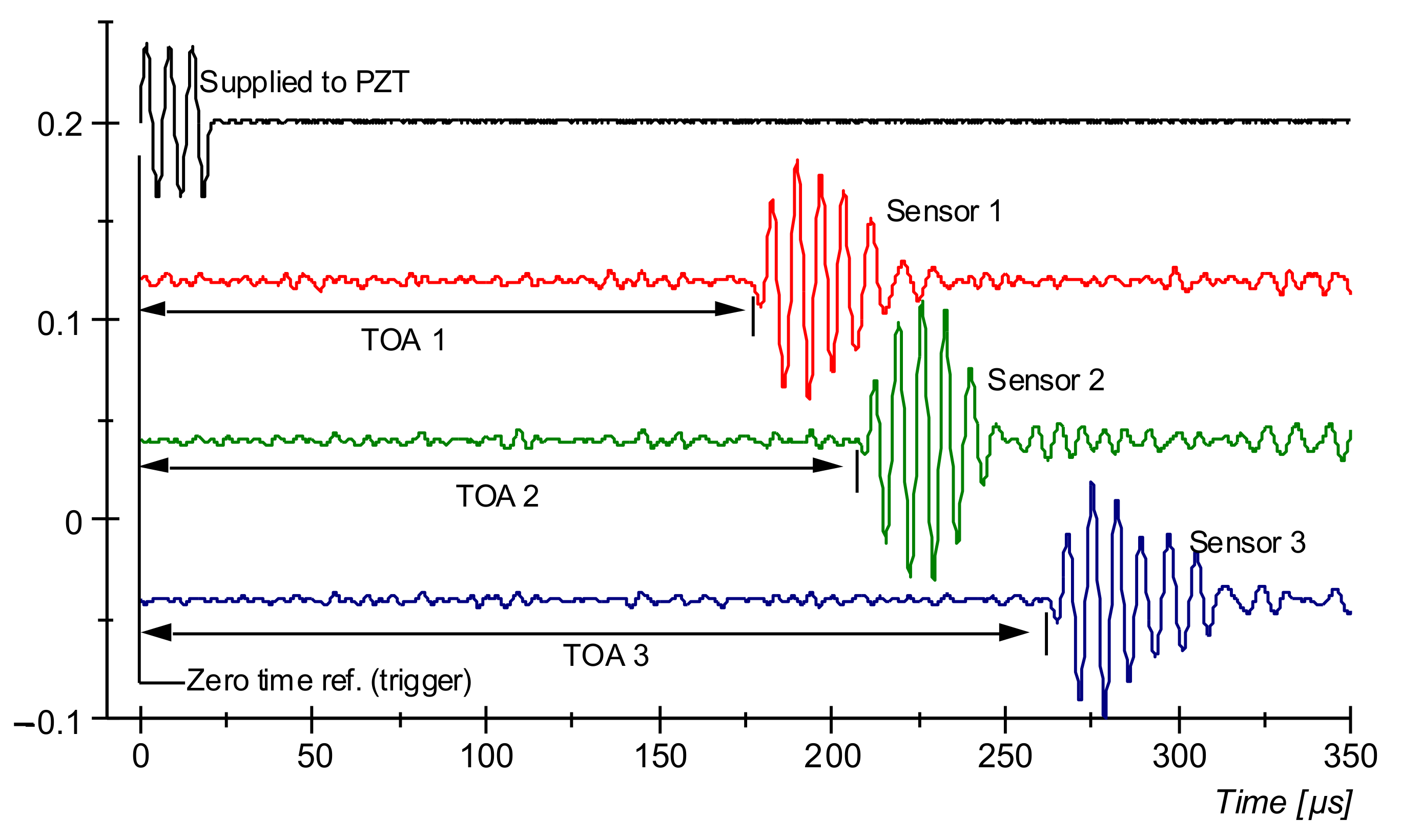
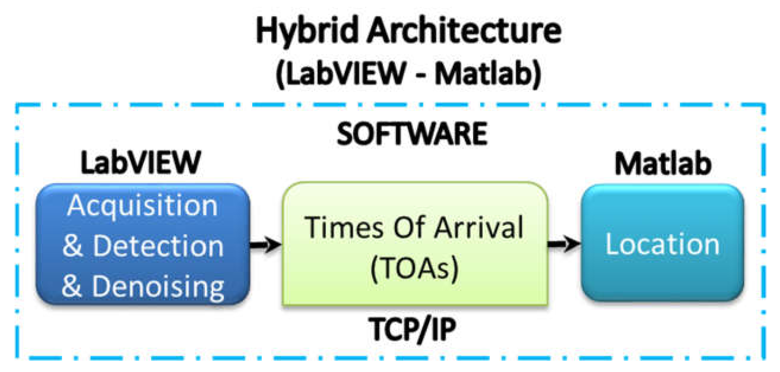
The multichannel instrumentation system has a specific hardware of acoustic signal conditioning and acquisition (PXI-National Instruments), and several software blocks for detecting and locating the acoustic signals. Figure 11 shows the general block diagram of the hybrid processing system for the detection of AE and the localization of the AES (hybrid architecture). It is formed by two parts; the first one is programmed in LabVIEW and it is devoted to the detection process. The acquisition of the acoustic signals is performed in all channels simultaneously and a signal processing of each channel is applied, which is based on digital filtering and wavelet denoising [13]. As a result of the processing, the time of arrival (TOA) is obtained by the first stage for each and every channel and each acoustic emission event. Other information can also be extracted, such as the amplitude of the AE.

The second part is programmed in Matlab and it is dedicated to locating the AES. It solves the equations system of trilateration for a 3D model of localization. The communication between both parts (from LabVIEW module to Matlab module) is mainly in terms of the information contained in the TOAs. It is performed efficiently through a packet transfer protocol. Particularly, TCP/IP is used (TCP/IP is short of Transmission Control Protocol/Internet Protocol (TCP/IP). A real-time localization of the AES is obtained by these means. In addition, remote data analysis is provided by this communications protocol.

This strategy reduced the computational and complexity costs because each nodule is dedicated to the tasks that optimize the acquisition and real-time parallel processing (DAQ and LabVIEW) and the iterative and non-iterative algorithms of localization (Matlab). High resolution is achieved with the DAQ and LabVIEW stage (>3.5 decades amplitude span, <0.02 μs time resolution, real-time digital band-pass filtering and wavelet filtering) and accuracy is improved with the Matlab stage (PSO algorithm).

4.2. Analysis of the Error Propagation to the Location of the AES

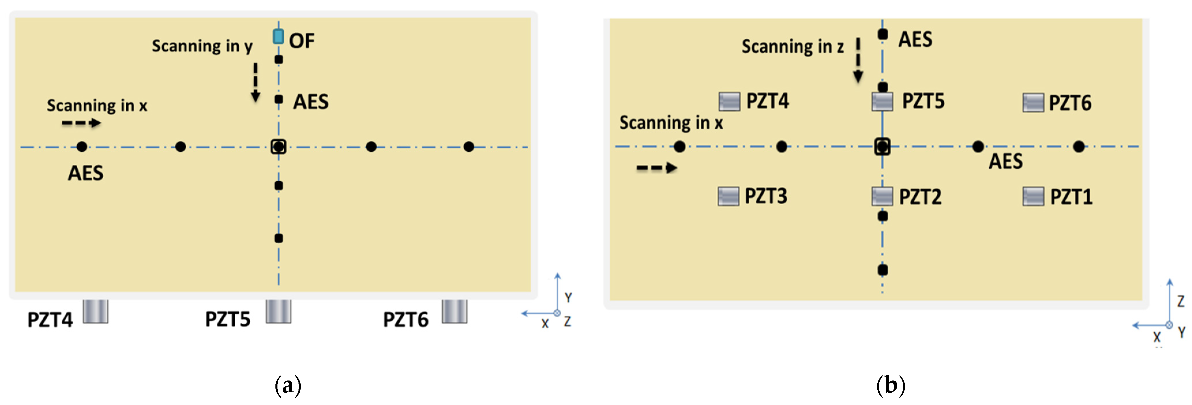
A simulation study was performed in order to evaluate what the influence of the error in the TOAs is on the accuracy of the location. For that, on the one hand, a sweep of the position within the tank was realized by moving the AES along the axis XYZ as shown in Figure 12. On the other hand, different percentages of error were added to the TOAs.

The results of the PSO method applied to the analysis of error propagation are shown below. It was the selected method that obtained the best response in a previous comparison without additional delay errors [24]. INI provided a similar performance (accuracy of 14 mm at the same cost), whereas the direct methods (Solve, LS, LN and Cramer) provided poor performance compared with PSO and INI (offset error of 143 mm and dispersion error of 30 mm) [24].

For each location of the AES, 100 samples were taken. In order to present and analyze the results, an offset error and a dispersion error have been defined as follows.

The offset error is the distance between the real position of the AES and the mean value of the solutions of location:

$$OffsetError=\sqrt{{\left(x_R-x_M\right)}^2+{\left(y_R-y_M\right)}^2+{\left(z_R-z_M\right)}^2},$$

(4)

where (x_R, y_R, z_R) are the coordinates of the real position of the AES and (x_M, y_M, z_M) are the mean value of the solutions.

The dispersion of solutions is quantified as the STD (σ) of the solutions of location:

$${\sigma }^2={\sigma }_x^2+{\sigma }_y^2+{\sigma }_z^2, \sigma =\sqrt{{\sigma }_x^2+{\sigma }_y^2+{\sigma }_z^2},$$

(5)

where σ_x, σ_y and σ_z are the STD of each axis.

Both errors are presented as a ratio (percentage) to the diagonal of the tank (3-D space dimensions), which is the maximum distance between two points inside it:

$${\%}_{Error}=\frac{Error}{D_{Tank}}·100,$$

(6)

where D_Tank is the diagonal:

$$D_{Tank}=\sqrt{D{x}^2+D{y}^2+D{z}^2}=1117.77\mathrm{mm},$$

(7)

where (Dx, Dy, Dz) = (900, 550, 370) mm are the dimensions of the tank.

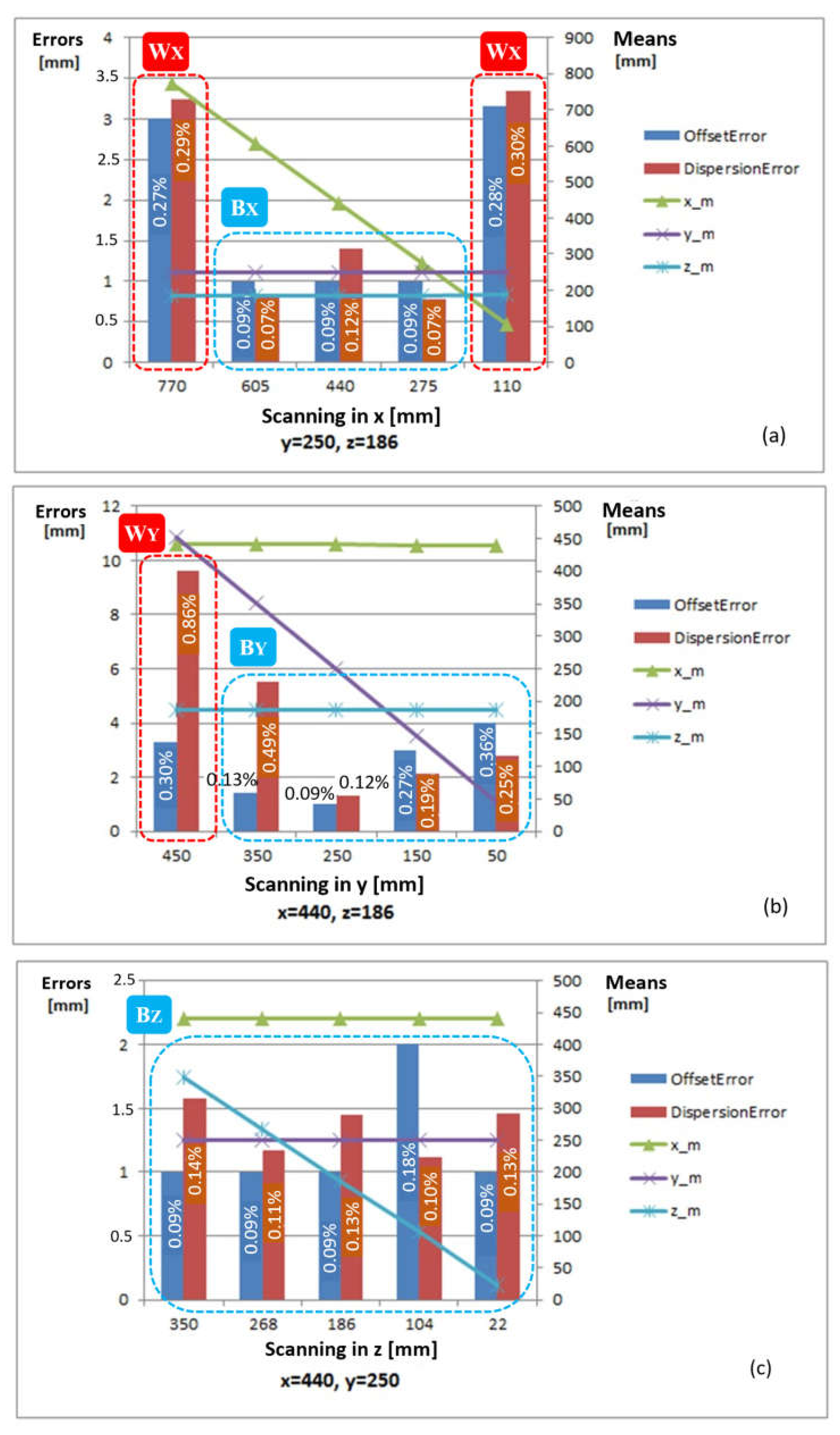
First, a random error up to 2% (standard uniform distribution—mean = 1%) was applied to each and every TOA. The results are shown in Figure 13. The mean solution for each coordinate, the offset error, the dispersion error and the percentage of each error is represented.

These results show different axis-dependent zones. The Bk areas are zones with a small limited stable error and the Wk areas are zones in the borders that exhibit higher errors. Edge and depth effects are observed in the zones Wx and Wy, respectively. In this case, the maximum dispersion error is 9.5 mm and the maximum offset error is 4 mm (less than 1% in both cases).

Second, a more intense error source (up to 10%—standard uniform distribution—mean = 5%) was applied. The results are similar to the previous case except for the scale. The results of 10% follow the same pattern as those of 2% with a factor of about 5. However, in the second case, the effect of the proximity to the PZT sensors is more pronounced (Wy area). The maximum dispersion error is 4.5 cm and the maximum offset error is 3.5 cm (less than 5% in both cases).

4.3. Evaluation of the Location Error with OF Internal Sensors

The same test bench (Section 4.2) is used here in order to generate AE at different positions inside the tank and find the location of the source using the multichannel fiber-optic instrumentation system. The same type of AE used in previous tests (Figure 8) is generated in this experiment but the AE source is placed at known positions inside the tank, making a sweep in the X axis so that there are 10 cm between two adjacent positions of the source, as shown in Figure 14.

Since the condition provided by the test bench is equivalent to a good scenario (low background noise, stable environment conditions, etc.), which is not the case in a real application, noise was intentionally introduced into the TOA measurements of each channel in order to emulate a realistic scenario. The maximum amplitude of the added noise is 30 µs, which, taking into account the velocity of the AE in water (1.49 mm/µs @ 25 °C), corresponds to a deviation of ±2 cm (2% of the maximum dimension of the tank). A series of ten measurements were taken at each position of the AE source. Moreover, the sweep covers a distance of 80 cm along the X axis.

The calculated positions of the AE source are presented in a 3D plot in Figure 15. It can be seen that there is a dispersion of the calculated positions of the AE source, which increases when it is close to the extremes of the tank (at the beginning and the end of the sweep).

This can be observed in more detail in Figure 16, where some statistical characteristics of the results obtained are shown.

This behavior is attributed to the degradation of the signal to noise ratio with the increasing distance from the AE source, because when the AE source is at one extreme of the tank, the SNR of the sensor placed farther away (at the opposite side of the tank) decreases considerably. Based on these results, it can be concluded that the system has a better performance, regarding the location of the source, for the motorization of the zones placed in the middle of the tank. In addition, under the condition of this test, the system is able to calculate the position of the AE source with precision <5 cm in each axis and 6 cm of accuracy. However, it can be seen from Figure 16 that the most repeated calculated position (mode of the sample) corresponds with the right position in all cases. This suggests that, in practical applications, a simple statistical analysis based on the mode calculation over a series of measurements can be used in order to improve the performance of the system when measurements are taken under unfavorable conditions.

5. Discussion

Based on previous results, the Particle Swarm Optimization strategy of localization was demonstrated as the most efficient in terms of computational, complexity costs and performance in laboratory conditions of measurement [24]. The Indirect Non-Iterative method provided a similar performance (less offset error but double dispersion error) at the same cost, whereas the other localization algorithms (direct methods Solve, LS, LN and Cramer) provided poor performance compared with PSO and INI (seven times worse offset error and four times worse dispersion error). Therefore, we focus here on the results with PSO.

A new study that was not in previous studies deals with the analysis of the error propagation from the arrival times to the location results. The delay errors from the PD source to each acoustic sensor are modeled here as a random distribution (from 1% to 5% mean error, up to 10% maximum error). The origin of these errors in real conditions are of a different nature: (I) the PD source is a small region of the solid isolator and not a systematic point; (II) the conditions of propagation can change even for consecutive detections of the same acoustic source (mainly due to temperature fluctuations); (III) amplitude noise affects the effectiveness of the amplitude threshold that triggers the detection and this has a higher impact with a lower signal to noise ratio in the detector (this depends both on the AE intensity and on the attenuation path); and (IV) the amplitude of each single AE is variable for a characteristic PD activity (this depends on the specific intensity of each discharge event within a PD area and on the acoustic path along this area). It is worth mentioning that these errors are mitigated with the use of internal sensors (fiber-optic sensors), because the trajectories are more direct and there are fewer interfaces among materials (coils/paper/oil/metal) present; in particular, the oil/walls interface is removed.

The strategy of propagating errors was applied by adding random additional delays artificially between the first stage of detection and the second stage of localization (this last was reduced to the case of PSO). In addition, the tests were carried under different conditions of error magnitude (1 and 5% mean error) and positions of the acoustic source. The edge, depth and proximity effects were clearly identified during the analysis of the location results. Even so, the maximum relative errors of location (offset and dispersion) are limited to less than the TOA relative mean errors. Results of locations better that 1 cm in 1 m were obtained with TOA uniform (0–2%) error distribution. These results are scaled proportionally five times for the case of 0–10%. It can be concluded that the location algorithm reduces the relative error for small variability of the delays to multiple sensors (first case, 1%); that is, the propagation of the error is a second order moment (random errors) and it is concentrated on the delays to the sensors with better detectability when there is an excess number (>3 sensors plus a reference for 3D location). However, when the variability of the delays is intense (second case, 5%), it is dominant in the location error, obtaining relative errors of the same order both in the offset (deviation from the real position) and in the dispersion of the values (precision); that is, a direct translation can be deduced from the relative error in the time of arrival to the relative error in the location. Finally, when the source is within zones at the edges (about 25% of the volume that is close to the walls), the results show higher errors than in the central region. Edge and depth effects are seen as location errors two to three times worse than in most and general cases. Therefore, for the PD sources in the central volume (75% of the volume), the location errors are even better than those reported of 10 mm.

Experimental tests with three internal OF sensors have shown that a precision <5 cm and an accuracy of 6 cm are achieved when there are unfavorable conditions. However, a simple calculation of statistic mode can be used in order to improve the performance of the system to achieve a better than 10 mm accuracy. Additionally, the resolution of the system was obtained by measuring the background noise levels at channels. The results show a detection limit better than 10 Pa. However, this can be improved in order to achieve the objective of a 1 Pa resolution (limited by the 12 bit DAQ system).

The structure of real transformers is more complex than the developed simulation and test scheme in laboratory conditions [27]. However, there are results compared in both conditions (with simplified structures in a controlled laboratory environment and with real complex structures of transformers in the field) that show the representativeness of the models [21]. An alternative is to include in the localization algorithm a detailed physical model of the structure inside the transformer [26], where a variant of PSO is applied to search for the acoustic signal path (PSO Route Search).

On the other hand, additionally, in the case of transformers in the field, the usefulness and even the need for combined acoustic and electrical measurements is demonstrated. When acoustic measurements have internal sensors, the following benefits are achieved: either the sensor gives an improved location reference with a barrier-free direct detection, or this direct detection with multiple sensors provides the region where the high PD activity is located and, consequently, it locates the precursor to failure. The precision with which the acoustic emission source can be located will ultimately depend on the number of sensors distributed and their strategic location [28]. The systems presented in this work are scalable to a greater number of sensors and provide strategies to discard the worst located acoustic sensors to give location information, either because they are further away from the source, or in the case of being blinded by barriers in a more complex structure of the transformer.

An additional aspect is the impact of oil temperature on the speed of propagation. To adjust this parameter to the measurement conditions, it is recommended to include an estimate of the mean temperature inside the transformer [29] or to monitor it, using the same internal fiber optic sensor technology as for acoustic detection [30].

It is impossible to improve the acoustic signal to noise ratio by averaging or to reduce the noise bandwidth with synchronous detection, because the AE signals generated by PD are transient and of a non-persistent nature. Therefore, we focus on reducing noise individually in each detected signal by wavelet filtering and narrowing the noise bandwidth. Although in this work we have not used classification techniques to cluster noise and phantom signals, this post-processing can be applied, either as a phase-resolved partial discharge (PRPD) acoustic pattern [31,32] or with other approaches to signal and noise classification [33,34].

6. Conclusions

The detection of acoustic emissions with multiple channels and different kinds of sensors (ultrasound electronic sensors and optical fiber sensors) has been implemented in a modular configuration, thus, it is easily adapted to different applications. The source localization based on times of arrival was also implemented and analyzed, by comparing different strategies for solving the location equations. For that, a hybrid programming architecture has been proposed and demonstrated. It is composed of a virtual instrumentation system for the acquisition and detection of multiple acoustic channels, an algorithms-oriented programming system for the implementation of localization techniques and a communication module between them that is performed by a packet transfer protocol that allows remote operation.

A location algorithm based on the measurement of the time of arrival of the acoustic signals was applied to the scenario of three internal fiber-optic sensors. Each sensor is used for the AE monitoring of an area and all sensors are involved along with a zero time reference for locating the source of AE. Additionally, a systematic analysis of location errors is included. Results show that the system is accurate to 6 cm with a precision better than 5 cm under conditions of noise equivalent to a 2 cm deviation that was added to the measurements of each sensor. Moreover, using a simple statistic mode calculation over a series of measurements enables the location of the AE source with an accuracy of 1 cm.

For the first time, the delay errors are modeled and error propagation is applied with the source of errors and the localization algorithms. This is thanks to the two stages architecture that optimizes the design of the system in terms of hardware/software complexity, time processing cost and precision. High resolution is achieved with the DAQ and LabVIEW stage of the system (>3.5 decades amplitude span, <0.02 μs time resolution, real-time digital band-pass filtering and wavelet filtering) and accuracy is improved with the Matlab stage (PSO algorithm) in terms of localization errors (dispersion and offset of the calculated location). Both stages are designed to communicate continuously, thus instead of other post-processing approaches, we integrate the overall signal processing and algorithms for real on-line operations. On the other hand, this error analysis was extended to the fiber-optic sensing systems of multiple channels (note that the OF sensors of PD are mainly reported as individual units).

References

1. IEEE. IEEE Guide for the Detection and Location of Acoustic Emissions from Partial Discharges in Oil-immersed Power transformers and Reactors. IEEE Stand. 2007, 127, C57. [Google Scholar]
2. Wang, M.; Vandermaar, A.J.; Srivastava, K.D. Review of condition assessment of power transformers in service. IEEE Electr. Insul. Mag. 2002, 18, 12–25. [Google Scholar] [CrossRef]
3. ASTM. Standard Guide for Application of Acoustic Emission for Structural Health Monitoring. In Active Standard ASTM E2983–14; American Society for Testing and Materials (ASTM): West Conshohocken, PA, USA, 2019. [Google Scholar]
4. Wang, Q.; Hong, M.; Su, Z. An In-Situ Structural Health Diagnosis Technique and Its Realization via a Modularized System. IEEE Trans. Instrum. Meas. 2015, 64, 873–887. [Google Scholar] [CrossRef]
5. AMSY-6 of Vallen Systeme. Available online: http://www.vallen.de/products/multi-channel-systems (accessed on 20 August 2021).
6. LAN-XI of Brüel & Kjær. Available online: http://www.bksv.com/Products/frontends/lanxi (accessed on 20 August 2021).
7. PXI of National Instruments. Available online: http://www.ni.com/pxi/esa/ (accessed on 20 August 2021).
8. Yongfen, L.; Xiaohu, X.; Fei, D.; Xiao, T.; Yanming, L. Comparison of DOA Algorithms Applied to Ultrasonic Arrays for PD Location in Oil. IEEE Sens. J. 2015, 15, 2316–2323. [Google Scholar] [CrossRef]
9. Song, L.; Cooper, K.L.; Wang, Z.; Wang, A.; Liu, Y. Position location of partial discharges in power transformers using fiber acoustic sensor arrays. Opt. Eng. 2006, 45, 114401. [Google Scholar] [CrossRef]
10. Posada-Roman, J.E.; Garcia-Souto, J.A.; Rubio-Serrano, J. Multichannel optical-fibre heterodyne interferometer for ultrasound detection of partial discharges in power transformers. Meas. Sci. Technol. 2013, 24, 094015. [Google Scholar] [CrossRef]
11. Kundu, P.; Kishore, N.K.; Sinha, A.K. Identification of two simultaneous partial discharge sources in an oil-pressboard insulation system using acoustic emission techniques. Appl. Acoust. 2012, 73, 395–401. [Google Scholar] [CrossRef]
12. Boya, C.; Ruiz-Llata, M.; Posada-Roman, J.E.; Garcia-Souto, J.A. Identification of multiple partial discharge sources using acoustic emission technique and blind source separation. IEEE Trans. Dielectr. Electr. Insul. 2015, 22, 1663–1673. [Google Scholar] [CrossRef]
13. Bua-Nuñez, I.; Posada-Roman, J.E.; Rubio-Serrano, J.; Garcia-Souto, J.A. Instrumentation System for the Location of Partial Discharges using Acoustic Detection with Piezoelectric Transducers and Optical Fiber Sensors. IEEE Trans. Instrum. Meas. 2014, 63, 1002–1013. [Google Scholar] [CrossRef] [Green Version]
14. Prasanta Kundu, N.; Kishore, K.; Sinha, A.K. A non-iterative partial discharge source location method for transformers employing acoustic emission techniques. Appl. Acoust. 2009, 70, 1378–1383. [Google Scholar] [CrossRef]
15. Lima, S.E.U.; Frazao, O.; Farias, R.G.; Araujo, F.M.; Ferreira, L.A.; Miranda, V.; Santos, J.L. Acoustic Source Location of Partial Discharges in Transformers. In Proceedings of the Fourth European Workshop on Optical Fibre Sensors. International Society for Optics and Photonics, Porto, Portugal, 8–10 September 2010; p. 76532N. [Google Scholar]
16. Tang, L.; Luo, R.; Deng, M.; Su, J. Study of Partial Discharge Localization using Ultrasonics in Power Transformer based on Particle Swarm Optimization. IEEE Trans. Dielectr. Electr. Insul. 2008, 15, 492–495. [Google Scholar]
17. Mirzaei, H.R.; Akbari, A.; Gockenbach, E.; Zanjani, M.; Miralikhani, K. A novel method for ultra-high-frequency partial discharge localization in power transformers using the particle swarm optimization algorithm. IEEE Electr. Insul. Mag. 2013, 29, 26–39. [Google Scholar] [CrossRef]
18. Posada-Roman, J.E.; Garcia-Souto, J.A.; Serrano, J.R.; Nunez, I.B. Multichannel ultrasound instrumentation for on-line monitoring of power transformers with internal fiber optic sensors. In Proceedings of the 2013 IEEE International Instrumentation and Measurement Technology Conference (I2MTC), Minneapolis, MN, USA, 6–9 May 2013; pp. 200–205. [Google Scholar]
19. Peiqing, M.; Xiuwei, L.; Yue, H.; Gehao, S.; Haifeng, Y.; Xiuchen, J. Acoustic-electrical based detection system for partial discharge localization of GIS. In Proceedings of the 2012 Power Engineering and Automation Conference, Wuhan, China, 18–20 September 2012. [Google Scholar]
20. Rubio-Serrano, J.; Garcia-Souto, J.A.; Posada-Roman, J.E. Instrumentation system and digital signal processing for studying the characteristics of the acoustic and electrical signals generated by partial discharges. In Proceedings of the 2012 IEEE International Conference on Industrial Technology, Athens, Greece, 19–21 March 2012; pp. 573–578. [Google Scholar]
21. Markalous, S.M.; Tenbohlen, S.; Feser, K. Detection and location of partial discharges in power transformers using acoustic and electromagnetic signals. IEEE Trans. Dielectr. Electr. Insul. 2008, 15, 1576–1583. [Google Scholar] [CrossRef]
22. Vakulya, G.; Simon, G. Fast Adaptive Acoustic Localization for Sensor Networks. IEEE Trans. Instrum. Meas. 2011, 60, 1820–1829. [Google Scholar] [CrossRef]
23. Ramírez-Niño, J.; Pascacio, A. Acoustic measuring of partial discharge in power transformers. Meas. Sci. Technol. 2009, 20, 115108. [Google Scholar] [CrossRef]
24. Bua-Nuñez, I.; Posada-Roman, J.E.; Garcia-Souto, J.A. Two-Stage Processing System for the Detection and On-Site Localization of Acoustic Emissions. In Proceedings of the 2015 IEEE International Instrumentation and Measurement Technology Conference (I2MTC) Proceedings, Pisa, Italy, 11–14 May 2015; pp. 1921–1926. [Google Scholar]
25. Posada-Roman, J.; Garcia-Souto, J.A.; Rubio-Serrano, J. Fiber Optic Sensor for Acoustic Detection of Partial Discharges in Oil-Paper Insulated Electrical Systems. Sensors 2012, 12, 4793–4802. [Google Scholar] [CrossRef] [Green Version]
26. Wang, Y.B.; Chang, D.G.; Fan, Y.H.; Zhang, G.J.; Zhan, J.Y.; Shao, X.J.; He, W.L. Acoustic localization of partial discharge sources in power transformers using a particle-swarm-optimization-route-searching algorithm. IEEE Trans. Dielectr. Electr. Insul. 2017, 24, 3647–3656. [Google Scholar] [CrossRef]
27. Wu, M.; Cao, H.; Cao, J.; Nguyen, H.-L.; Gomes, J.B.; Krishnaswamy, S.P. An overview of state-of-the-art partial discharge analysis techniques for condition monitoring. IEEE Electr. Insul. Mag. 2015, 31, 22–35. [Google Scholar] [CrossRef]
28. IEEE. Draft Guide for the Detection and Location of Acoustic Emissions from Partial Discharges in Oil Immersed Power Transformers and reactors. In IEEE PC57.127 Standards Draft; IEEE: Piscatway, NJ, USA, 2003. [Google Scholar]
29. Roslan, M.H.; Azis, N.; Kadir, M.Z.A.A.; Jasni, J.; Ibrahim, Z.; Ahmad, A. A Simplified Top-Oil Temperature Model for Transformers Based on the Pathway of Energy Transfer Concept and the Thermal-Electrical Analogy. Energies 2017, 10, 1843. [Google Scholar] [CrossRef] [Green Version]
30. N’Cho, J.S.; Fofana, I. Review of Fiber Optic Diagnostic Techniques for Power Transformers. Energies 2020, 13, 1789. [Google Scholar] [CrossRef] [Green Version]
31. Kunicki, M.; Cichon, A. Application of a Phase Resolved Partial Discharge Pattern Analysis for Acoustic Emission Method in High Voltage Insulation Systems Diagnostics. Arch. Acoust. 2018, 43, 235–243. [Google Scholar]
32. Ilkhechi, H.D.; Samimi, M.H.; Yousefvand, R. Generation of acoustic phase-resolved partial discharge patterns by utilizing UHF signals. Int. J. Electr. Power Energy Syst. 2019, 113, 906–915. [Google Scholar] [CrossRef]
33. Rubio-Serrano, J.; Rojas-Moreno, M.V.; Posada, J.; Martínez-Tarifa, J.M.; Robles, G.; Garcia-Souto, J.A. Electro-acoustic detection, identification and location of partial discharge sources in oil-paper insulation systems. IEEE Trans. Dielectr. Electr. Insul. 2012, 19, 1569–1578. [Google Scholar] [CrossRef]
34. Ardila-Rey, J.A.; Montaña, J.; De Castro, B.A.; Schürch, R.; Ulson, J.A.C.; Muhammad-Sukki, F.; Bani, N.A. A Comparison of Inductive Sensors in the Characterization of Partial Discharges and Electrical Noise Using the Chromatic Technique. Sensors 2018, 18, 1021. [Google Scholar] [CrossRef] [Green Version]
Figure 1. The instrumentation system based on OF and PZT sensing.
Energies 14 07873 g001
Figure 2. Multichannel acquisition and conditioning system.
Energies 14 07873 g002
Figure 3. Single OF sensor.
Energies 14 07873 g003
Figure 4. Detection optical interferometer of a single channel.
Energies 14 07873 g004
Figure 5. Detection optical interferometer of four channels.
Energies 14 07873 g005
Figure 6. Schematic of time differences with unknown time reference T.
Energies 14 07873 g006
Figure 7. Position location of the AE source based on TOA measurements and trilateration.
Energies 14 07873 g007
Figure 8. Typical AE signal detected by the system using three sensors and the TOA related each of them.
Energies 14 07873 g008
Figure 9. Acquisition and digital processing for TOA measurement and location of the AE source.
Energies 14 07873 g009
Figure 10. Detail of the acoustic characterization test bench.
Energies 14 07873 g010
Figure 11. Hybrid processing system for detecting and locating the AES.
Energies 14 07873 g011
Figure 12. Sweep of the AES position within the tank, scanning XY (top view) in (a) and scanning XZ (front view) in (b).
Energies 14 07873 g012
Figure 13. Results (2%) of the scanning X in (a), the scanning Y in (b) and the scanning Z in (c).
Energies 14 07873 g013
Figure 14. Experimental arrangement used for the location of the AE source in X axis sweep.
Energies 14 07873 g014
Figure 15. AE source location for a sweep in X axis.
Energies 14 07873 g015
Figure 16. Analysis of errors in the calculated standard deviations of the location for each axis: actual position, detected position (mean) and errors (std. deviation), as well as detected position reducing the dispersion error (mode); (a) in the Y axis, and (b) in the Z axis.
Energies 14 07873 g016