Abstract
The article presents research on the influence of the type of UHF antenna and the type of machine learning algorithm on the effectiveness of classification of partial discharges (PD) occurring in the insulation system of a power transformer. For this purpose, four antennas specially adapted to be installed in the transformer tank (UHF disk sensor, UHF drain valve sensor, planar inverted F-type antenna, Hilbert curve fractal antenna) and a reference log-periodic antenna were used in laboratory tests. During the research, the main types of PD, typical for oil-paper insulation, were generated, i.e., PD in oil, PD in oil wedge, PD in gas bubbles, surface discharges, and creeping sparks. For the registered UHF PD pulses, nine features in the frequency domain and four features in the wavelet domain were extracted. Then, the PD classification process was carried out with the use of selected methods of supervised machine learning. The study investigated the influence of the number and type of feature on the obtained classification results gained with the following machine-learning methods: decision tree, support vector machine, Bayes method, k-nearest neighbor, linear discriminant, and ensemble machine. As a result of the works carried out, it was found that the highest accuracies are gathered for the feature representing peak frequency using a decision tree, reaching values, depending on the type of antenna, from 89.7% to 100%, with an average of 96.8%. In addition, it was found that the MRMR method reduces the number of features from 13 to 1 while maintaining very high effectiveness. The broadband log-periodic antenna ensured the highest average efficiency (100%) in the PD classification. In the case of the tested antennas adapted to work in an energy transformer tank, the highest defect-recognition efficiency is provided by the UHF disk sensor (99.3%), and the lowest (89.7%) is by the UHF drain valve sensor.
Keywords:
UHF antenna; PD defect; power transformer; classification; machine learning; feature analysis; MRMR 1. Introduction
A defect in the insulation system is one of the main causes leading to a possible catastrophic failure of an electrical power device. Therefore, it is important that the condition of the insulation system is regularly verified during periodic tests or continuously using on-line partial discharge (PD) monitoring systems. Partial discharges are not only the main cause of damage to an insulation system but also a very reliable indicator of the formation of insulation defects in high-voltage electrical equipment [1,2].
The most frequently used methods of partial discharge detection, especially in field conditions, are the acoustic emission method and electromagnetic methods based on the registration of radio pulses in the HF, VHF, and UHF bands [3,4]. Moreover, in the case of devices with oil-paper insulation, the Dissolved Gas Analysis (DGA) method also plays an important role [5]. In the past decade, the UHF method in particular, has become the subject of numerous research and development activities. These works cover a wide range of issues such as: the development of new designs of UHF antennas [6,7,8], combined acoustic and electromagnetic PD sensors [9,10], new calibration methods for UHF partial discharge measurement [11], the use of UHF sensors to locate PD sources using time-difference of arrival (TDOA) [12], direction of arrival (DOA) [13,14], received signal strength indication (RSSI) [15,16], electromagnetic time reversal (EMTR) [17] and electromagnetic inverse filter (EMIF) [18] techniques, development of on-line PD monitoring systems [19], and automatic recognition of insulation defects based on advanced digital signal processing algorithms and machine learning methods [20]. The last issue is an important element of reliable diagnostics of electrical power devices because effective detection and identification of a defect (source of PD) can contribute to the prevention of a serious failure.
Most of the research works on the automatic classification of PD types focus on two issues, i.e., the selection and extraction of features describing PD signals and the implementation of machine learning (ML) methods. Among the numerous features describing PD, the most frequently selected and extracted are the statistical parameters (e.g., kurtosis, skewness, mean, variance, and cross-correlation factor) [21,22], two-dimensional phase-resolved partial discharge (PRPD) images [23], time-domain features (e.g., rise time, fall time, slew rate, pulse width) [24], frequency-domain features (e.g., mean amplitude of frequency, number of spectral peaks, root mean square value of frequency) [25], multifractal spectrum features [26], wavelet coefficients [27,28], and cross wavelet transform features [29].
The features mentioned above are used as input or training data in various PD pattern recognition methods, such as artificial neural network (ANN) classification [30,31], fuzzy clustering classification [32], distance-based classification [33], Fisher’s linear discriminant analysis (LDA) classification [34,35], classification based on the chaos theory [36], Bayesian classification [37], and support vector machine (SVM) classification [38].
In [39], the authors applied SVM for the classification of UHF signals emitted by PD occurring in gas-insulated switchgear (GIS). They achieved an average recognition rate of 90%, while using as features patterns based on chromatic parameters H, L, and S. In [40], the authors presented a design of a Hilbert fractal antenna applied for detecting and classifying PD types in an oil-paper insulated system. They used frequency components of the detected PD signal as features while considering the first 15 frequencies corresponding to the highest power peaks. They achieved a recognition rate of 95% when classifying the different PD types. In [41], the authors investigated defects of epoxy insulators using the UHF method. They extracted feature information from time-resolved partial discharge (TRPD) and PRPD analysis, while selecting them using minimal redundancy criterion (MRMR) and with SVM. They proposed a new algorithm for recognition reaching over 94% accuracy. In [42], the authors were involved in research using UHF measured with a wideband Horn antenna to detect and classify PD occurring on disc ceramic insulators. They applied ML techniques. As features they applied wavelet decomposition and statistical features. They used principal component analysis (PCA) and recursive feature elimination (RFE) for feature selection. In [43], the authors provided a review of various computational intelligence techniques applied for technical condition estimation in the field of power transformers. In addition, in a relatively recent study [44], the authors comprehensively summarized research on the area of detection, classification, and localization of UHF-recorded PD sources.
It must be admitted that a great deal of research has already been done, which confirms that there are a number of possibilities to classify PD types that were recorded with different types of antennas. Depending on the type of algorithm and the selected features, the authors have obtained efficiencies as high as 99.6%, as described in the review [44].
This article assesses the impact of the type of antenna used and the type of supervised ML algorithm on the effectiveness of PD classification in the insulation system of the power transformer. For this purpose, four antennas adapted for installation in the transformer tank were used in the research (UHF disk sensor, UHF drain valve sensor, Hilbert curve fractal antenna, and meandered planar inverted-F antenna). Additionally, a broadband log-periodic antenna was used, which was a reference for the other antennas. These antennas recorded the UHF signals generated by five types of PD occurring in the oil-paper insulation of the transformer, i.e., partial discharges in oil gap, partial discharges in oil, partial discharges in air bubbles in oil, surface discharges, and creeping discharges. For the recorded PD pulses, nine features in the frequency domain and four features in the wavelet domain were extracted. Among the available methods of supervised machine learning, six algorithms were selected, which are indicated frequently in the literature as promising: Bayes (BY), Tree (TREE), Ensemble (EN), K-Nearest Neighbor (KNN), Linear Discriminant (LD), and Support Vector Machine (SVM).
The most important contribution of the paper lies in the demonstration that there is no effect of antenna design on classification performance. Regardless of the type of antenna, an average efficiency above 89.7% was obtained. A second significant contribution to the knowledge of the UHF-recorded discharge diagnostics is that only the peak frequency needs to be computed in order to realize classification with high levels of accuracy, reaching the value of 99.7% for chosen defects.
This paper is organized as follows. Section 2 presents the types of tested defects (PD sources) and the parameters of the partial discharge measurement setup. This section also discusses the selection and extraction of features describing PD and the algorithms used for their classification. Section 3 presents the results obtained from single-feature analysis and feature analysis according to the MRMR algorithm. In this part, the obtained classification results were also assessed. General conclusions from the conducted research are included in Section 4.
2. Materials and Methods
2.1. Experimental Setup for Partial Discharge Measurements
As part of the experiment, five types of partial discharges were investigated, which most often occur in the oil-paper insulation system of power transformers, i.e., partial discharges in oil gap (PD1), partial discharges in oil (PD2), partial discharges in air bubbles (PD3), surface discharges (PD4) and creeping discharges (PD5). To generate PD pulses, electrode systems were used, the schematic diagrams and dimensions of which are shown in Figure 1. The electrode systems were placed in a cylindrical test chamber with a diameter of 150 mm and a height of 300 mm, made of organic glass and filled with TRAFO EN-type mineral oil (Orlen, Plock, Poland).
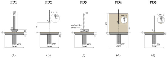
Figure 1.
Schematic diagrams of electrode systems for generating partial discharges in oil-paper insulation: (a) Partial discharges in oil gap. (b) Partial discharges in oil. (c) Partial discharges in air bubbles in oil. (d) Surface discharges on pressboard sample in oil with a negligibly small normal component of the electric field. (e) Creeping discharges (surface discharges on a pressboard sample in oil with significant normal component of electric field).
UHF sensors used in power transformers can be installed temporarily in standard oil drain valves, or permanently in specially adapted dielectric windows. The first type of sensor, due to the small diameter of the oil valve and the specific method of mounting, is, in most cases, a simple monopole antenna made in the shape of a straight rod, cone, or small disk [45,46,47]. The design of the second type of sensor is usually more sophisticated and is currently the subject of numerous research works aimed at developing a broadband UHF antenna that guarantees high sensitivity of PD detection and easy installation in a dielectric window. Apart from the first historically, but still popular (especially in commercial systems) narrowband disk antenna, broadband (or multiband) microstrip patch antennas are being implemented, e.g., the antipodal Vivaldi antenna [48], bio-inspired antennas [49,50], the Archimedean spiral antenna [51,52], the meander-line antenna [53], the spiral equiangular antenna [54,55], and various antennas based on fractal geometry, e.g., the Hilbert [56], Minkowski [57], and Peano fractal antennas [58].
In order to assess how the selection of a given antenna design affects the effectiveness of the PD classification process, the drain valve sensor and disk sensor type IC43 [59] (both produced by Qualitrol DMS, Glasgow, United Kingdom), Hilbert curve fractal antenna [60] and meandered planar inverted F-antenna [19] were selected for the purposes of the study. Additionally, the reference ultra-wideband log-periodic antenna type VULP 9118A (Schwarzbeck Mess-Elektronik OHG, Schönau, Germany) was used [61]. The parameters of the antennas used are summarized in Table 1, while the reflection coefficient S11 characteristics measured on the test stand using the vector network analyzer type KC901S (Deepace, Guangdong, China) are shown in Figure 2. In the remainder of this paper, references for each antenna are used as summarized in the left part of Table 1: A1–A5.

Table 1.
Parameters of UHF antennas used in the research.
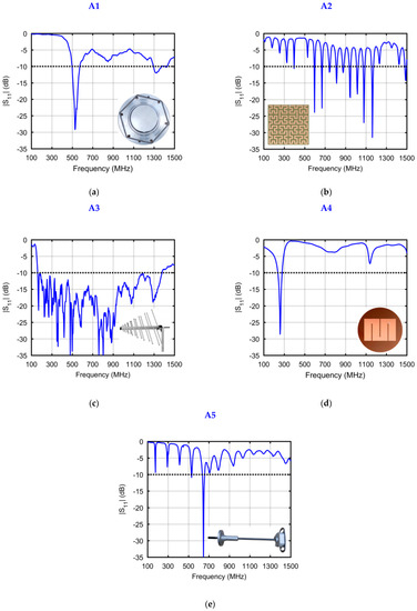
Figure 2.
The measured return loss (S11) characteristics of the antennas used in the tests: (a) Disk sensor type Qualitrol IC43; (b) Hilbert curve fractal antenna; (c) Log-periodic antenna type Schwarzbeck VULP 9118 A; (d) Meandered planar inverted-F antenna; (e) Qualitrol UHF drain valve sensor.
Measurement of PD in the UHF band was carried out in a shielded high-voltage hall with dimensions of 5390 × 2932 × 2499 mm, for which the theoretically determined main resonance frequencies for mode numbers m, n, p ∈ {0, 1, 2} are in the range from 58 MHz for transverse electric mode TE101 to 158 MHz for transverse magnetic mode TM220. For this reason, and the fact that the maximum operating frequency of the antennas used did not exceed 1500 MHz, the PD signals recorded by the antennas were filtered with a bandpass filter of 150 MHz to 1500 MHz. The antennas were placed at a distance of d = 2 m from the partial discharge source, thanks to which the far-field condition was fulfilled, such that d ≥ 2L2/λ where d is the distance from the source of UHF PD signals to the receiving antenna, L is the largest dimension of antenna aperture, and λ is the wavelength.
UHF pulses from PD were recorded with a digital oscilloscope of the MDO3104 type (Tektronix Inc., Beaverton, OR, USA) with a sampling rate of 5 GS/s. A high-frequency current transformer of the RFCT-4 type (Dimrus, Perm, Russia) was used to trigger the PD pulse acquisition process, installed on the grounding conductor of the electrode system. In addition, the intensity of PD and the level of their apparent charge q were monitored using a conventional partial discharge meter (PD-Smart, Doble Engineering Company, Marlborough, MA, USA) according to IEC 60270 standard [62]. All measurement system components are shown in Figure 3, while the basic parameters of the tested types of partial discharges are summarized in Table 2.
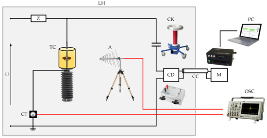
Figure 3.
Schematic diagram of the measurement setup: U—high-voltage supply; Z—short-circuit current limiting resistor; TC—oil filled test chamber with electrode system for generating partial discharges; A—antenna; CK—coupling capacitor; CD—coupling device (measuring impedance); CC—connecting cable; M—conventional partial discharge measuring device; PC—computer; OSC—digital oscilloscope; LH—shielded high-voltage laboratory hall.
Table 2.
Parameters of the investigated types of partial discharges.
2.2. Selection of Features and Classification Method Applied
In the process of selecting features describing UHF PD pulses, both their high efficiency in applications related to automatic pattern recognition, as well as the possibility of their fast calculation with the use of FPGA technology were considered. This technology is more and more often implemented in modern systems of detection and online monitoring of PD [19,63,64,65,66]. Its popularity is due to the fact that it allows for processing signals and performing calculations in real time. Because of this, the online PD monitoring system is able to quickly detect and identify the type of defect and thus can reliably assess the threat and prevent a dangerous failure of the power electrical device. The latest FPGAs implement not only very efficient algorithms of the fast Fourier transform (FFT), but also more complex algorithms of digital signal processing, such as discrete wavelet decomposition [67,68,69]. For this reason and based on a literature search concerning classification problems in machine learning, we decided to select 9 features determined in the frequency domain (peak frequency, weighted peak frequency, spectral centroid, spectral roll-off frequency, spectral skewness, spectral kurtosis, and partial power determined for three frequency ranges) [70,71,72] and 4 features in the wavelet domain (energy of details coefficients at four decomposition levels) [73]. Descriptions of selected features along with references to mathematical formulas are summarized in Table 3, and Figure 4 shows their graphical representation.
Table 3.
List and description of selected features.
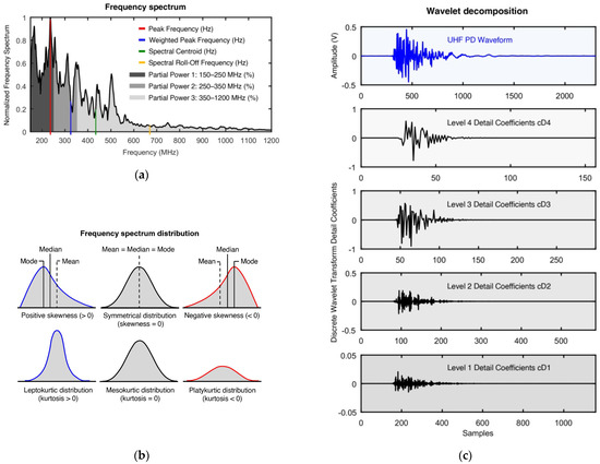
Figure 4.
Graphical representation of the selected features used in the machine learning process: (a) Frequency-domain features (peak frequency, weighted peak frequency, spectral centroid, spectral roll-off frequency, partial powers); (b) Higher-order statistical features in the frequency domain (skewness and kurtosis of the frequency spectrum); (c) Wavelet-domain features (energy of details coefficients of a discrete wavelet transform calculated at four decomposition levels).
In Figure 5 and Figure 6, selected sample scatter plots are presented along with box plots that encapsulate the basic information of descriptive statistics. The presented relationships illustrate the dependence of the feature F8 relative to F2 and F11 relative to F1, respectively; the UHF signal was measured using the A1 antenna. Different colors and markers were used to indicate the values obtained for each class PD1-PD5. The choice of visualization was made for two extreme cases: (1) the existence of visually distinct clusters while correlations between features exist, and (2) the absence of distinct clusters for all classes while no correlations between features exist. Box plots allowed us to determine the variability of values across groups. It is assumed that a large variation in box plots can be an indicator of the potential use of a feature, or set of features, for prediction. To enhance the process of analyzing all possibilities, the process was automated using scripts written in a MATLAB environment.
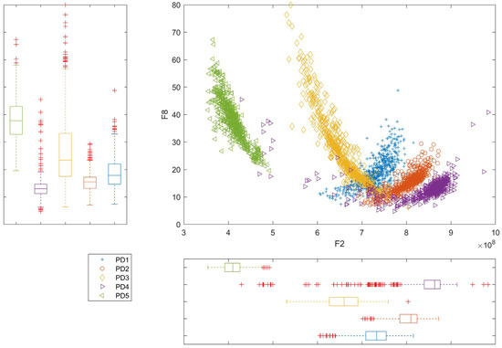
Figure 5.
Example scatter plot of the F8 versus F2 features along with box plots for data acquired from antenna A1, showing clearly distributed clusters and significant correlation of F8 vs. F2.
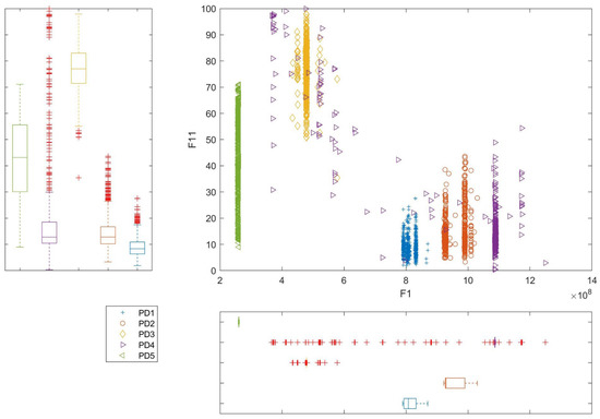
Figure 6.
Example scatter plot of the F11 versus F1 features along with box plots for data acquired from antenna A1, showing less clearly distributed clusters and no correlation of F11 vs. F1.
Based on the analysis of all possible combinations of each relationship, some features were found to correlate strongly, while others showed no correlation. The calculated features were examined for the existence of correlations between them before proceeding to classification. Pearson and Spearman correlation coefficients were calculated, providing very similar results. We then calculated how many times a feature was or was not correlated. In particular, results were grouped for highly correlated features (no HCF), where |r| > 0.7 and uncorrelated features (no UCF), where |r| < 0.3. The results are presented in Figure 7 and Figure 8 for the five considered antennas (as separate plots) and the various PD classes (in a different color).
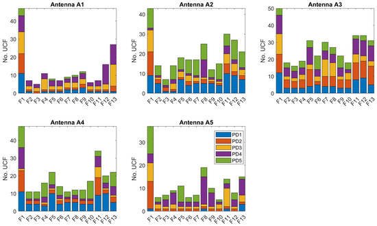
Figure 7.
The number of times a given feature was uncorrelated (no UCF) with another: |r| < 0.3.
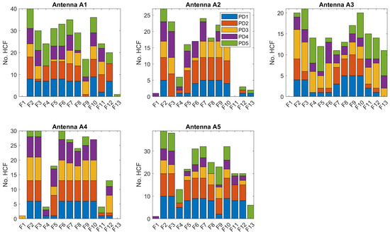
Figure 8.
The number of times a given feature was highly correlated (no HCF) with another: |r| > 0.7.
Analysis of the total number of UCF > 25 indicates that the following features might be used for classification: F1 and F13 for A1; F1, F8, F11, F12 for A2; F1, F5, F7, F8, F11, F12, F13 for A3; F1, F11 for A4; and only F1 for A5. In contrast, it can be shown based on Figure 8 that feature F1 does not correlate strongly with any other feature in most cases and for each antenna type. Furthermore, the value of HCF < 10 indicated that F4 does not correlate strongly for A2 and A3; F11 for A2 and A4; F12 for A2; and F13 for A1, A2, A4, and A5. To sum up, we can state that the best results should be obtained for F1 and possibly for individual antennas also: for F4, F11–F13.
Feature selection is one of the fundamental problems in classification issues that data scientists face. The feature selection process is primarily used to reduce the model size and dimensionality, secondly to prevent overfitting, and in tertiary but not last, to improve interpretability. These advantages should provide the best predictive power when modeling a given dataset.
There are a number of methods that are commonly used, such as independent component analysis (ICA) [74], principal component analysis (PCA) [44], minimum redundancy maximum relevance (MRMR) algorithm [75,76], and neighborhood component analysis (NCA) [77]. Many authors reduce feature sets to a few dimensions using some of the aforementioned methods, e.g., [78,79,80].
In order to determine which features are important in the classification process of our particular problem, the MRMR method was applied. Using the method, predictor importance score (PIS) values can be determined, with the highest values indicating the most optimal features. The PIS values calculated for individual antennas are visualized in the form of a bar chart in Figure 9. The MRMR algorithm is deterministic, and each time it is called it gives the same results.
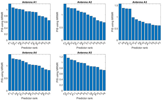
Figure 9.
PIS values calculated using the MRMR algorithm for the five considered antenna.
The results obtained found that each time the first feature has a relatively significantly higher value than the second and subsequent features. For antenna A1, A2, A3, and A4, it was feature F1, while for antenna A5, it was feature F3. The second and subsequent positions were occupied by different features, depending on the type of antenna. For antenna A1, only two features obtained PIS values above 1, while for the other antennas, features with PIS factors above 1 were obtained by significantly more features. The above indicates that a single feature allows class prediction with high accuracy.
3. Results and Discussion
3.1. Single Feature Analysis
We tested the classification performance separately for each of the F1–F13 features in the first step. For the algorithms considered, the classification process was performed using cross-validation with a k-fold parameter value of 20. The performance values in the validation process are summarized as a stacked bar plot in Figure 10, where the values obtained for each antenna are shown in different colors and for different algorithms as separate drawings.
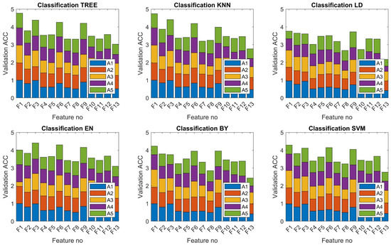
Figure 10.
Stacked bar plot depicting validation accuracy values gathered for particular antenna types and features for the selected classification method.
From the images shown, one can read the variation in classification performance when applied separately. In order to quantitatively assess the quality of prediction when using successive features separately, the average accuracy values obtained for each feature and the selected algorithms are summarized in Table 4. Based on the tabulated data analysis, it was found that the use of feature F1 for the TREE and KNN algorithm allows for classifications with efficiencies exceeding 94%. On the other hand, features F3, F6 and F9 also receive relatively good results when applied alone, achieving accuracies exceeding 80%.
Table 4.
Summary of averaged accuracy for five antennas for each feature applied individually.
In our opinion, the high efficiency obtained for the F1 feature results in the fact that it is the only one that does indicate a lack of correlation with the other features, while the other features, depending on the type of antenna, correlate with each other. It can also be deduced from Table 4 that by far the best results were obtained for the TREE and KNN algorithms.
In Table 5, the averaged accuracies obtained for particular algorithms regardless of the feature applied are summarized.
Table 5.
Average accuracies calculated for all features applied in classification.
3.2. Feature Analysis According to MRMR
In the next step, the classification process was carried out using a cumulative set of features, starting with the first one indicated by the MRMR method, then the first two, the first three, etc. Then the classification efficiencies were calculated for the six algorithms considered. The obtained results are included in Figure 11 in the form of a stacked bar plot, which illustrates the cumulative effectiveness values obtained for the successive antennas (marked with different colors) and the considered algorithms (subsequent figures).
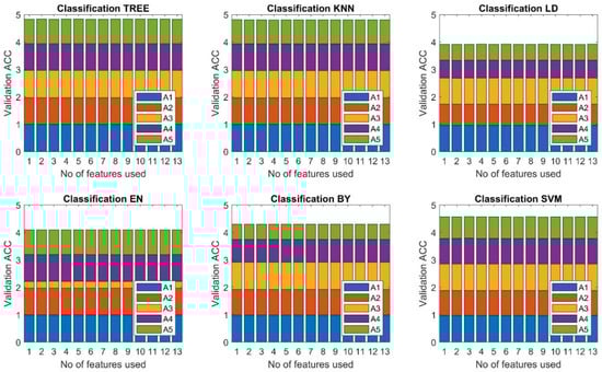
Figure 11.
Stacked bar plot depicting validation accuracy values gathered for particular antenna types and algorithms when using various No of features according to MRMR method.
Based on the gathered outcomes, very poor results were obtained for the EN algorithm for antenna A3. Worse results were also obtained for the LD algorithm, where weaker accuracies were calculated for antennas A4 and A5. Relatively good metrics were calculated for the other algorithms. From the relationships illustrated in Figure 11, it can also be concluded that after applying the first and subsequent features indicated by the MRMR method, there is no statistically significant difference in the obtained efficiencies. This clearly shows that applying only the first feature is sufficient to obtain almost the highest rates. In order to evaluate the quality of the classification and extract the best algorithm, the average efficiencies for all antennas were calculated, and these values are summarized in Table 6. It can be read from the table that, on average, the highest value, which was 96.8%, was obtained for the TREE algorithm when using two features. Slightly lower efficiencies characterized the KNN and SVM algorithm, which exceeded 90%. It should be noted that these results are not the same as in Table 4, because there the classifier predicted PD class based on the same feature, while here these, indicated by the MRMR, were applied. Hence, the average values are higher than those presented in Section 3.1.
Table 6.
Average over accuracies calculated while using various No of features.
The arithmetic means for the algorithms were also calculated regardless of the number of features used, and similar results were obtained for the same three algorithms. The values are summarized in Table 7. Again, the best results, above 90%, were obtained for the TREE, KNN, and SVM algorithms. Using two features during the prediction of the PD class resulted in a 1.4% improvement in accuracy.
Table 7.
Average over accuracies calculated for particular algorithms.
3.3. Evaluation of Classification Performance
For classification performance evaluation, it is common to use various score metrics, e.g., accuracy (ACC) (1), precision, recall, or F1-score (2), just to name the most popular ones, calculated based on the confusion matrix. However, these measures do not provide the complete picture of the performance and may give overly optimistic inflated results, especially in cases where the considered dataset is class-imbalanced [42]. The Matthews correlation coefficient (MCC) [81] (3) is a more reliable measure that estimates a high value only in cases when the classifier obtained appropriate scores for all the confusion matrix elements—true positives (TP), false negatives (FN), true negatives (TN), and false positives (FP)—proportionally both to the size of negative and positive elements in the dataset. The Cohen’s Kappa statistic [82] (4) is appropriate for both multi-class and class-imbalanced issues. This coefficient indicates how much better a classifier is performing compared to a simple classifier that simply guesses.
where: TP, TN, FP, FN is the No of correct or incorrect classified samples, —observed agreement, —expected agreement.
Figure 12 shows the confusion matrices for each antenna obtained for the TREE algorithm, which obtained the best results, when applying the first feature according to the MRMR method. From the matrix, it can be seen which classes of discharges performed better and which performed worse in the classification process. It was found that efficiencies above 99.7% were obtained for class PD1 recorded with antennas A1 and A3 and class PD2 with antennas A1, A2 and A3, and class PD5 was 100% effective regardless of the type of antenna. Discharges of type PD3 and PD4 only for antenna A3 received a high efficiency ratio. Based on the matrix analysis, it is also clear that the highest efficiency was obtained for signals recorded with antenna A3, then A1, A2, and A4. The classification results for data obtained with antenna A5 were the lowest but also relatively high, exceeding 89%.
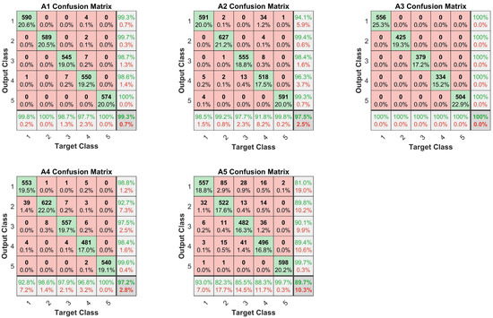
Figure 12.
Confusion matrices for the TREE algorithm and first MRMR feature.
Table 8 comparatively summarizes the F1-score, MCC and Kappa parameter values calculated for the classification process using the TREE algorithm with a single feature, according to the MRMR method. It can be seen that the ACC values are almost identical to the F1-score values. The MCC values are slightly smaller, in the range of 0.002 to 0.024. In contrast, as compared to MCC, the Kappa values are significantly lower, in the range of 0.014 to 0.194. The worst predictions were obtained for the feature set calculated from the signals recorded with the A5 antenna, for which the Kappa is only 0.68. The best predictions were gathered for the A3 antenna, reaching the highest score values of 1.
Table 8.
Goodness parameters of the TREE algorithm applied to first MRMR feature.
4. Conclusions
As part of the research work, the results of which are presented in this paper, UHF signals were measured with five types of antennas. The UHF signals were emitted in systems modeling partial discharges of five different types. The study attempted to extract features that were used for classification using supervised learning methods. The most crucial conclusions, which were stated based on the analyses performed, are as follows:
- Relatively high scores of efficiency measures were calculated for the feature representing peak frequency (F1). When applied as a predictor using the TREE and KNN algorithm, it allowed for classifications with accuracy exceeding 94%.
- Application of features F3, F6, and F9 resulted in accuracies exceeding 80%.
- Application of the MRMR method enabled reduction of the number of features from 13 to 1 while maintaining very high effectiveness. Best scores were achieved for two features.
- The highest efficiency (100%) was obtained for the broadband log-periodic antenna intended for research purposes. Comparably high efficiency of defect recognition was obtained for antennas installed in the dielectric window of the transformer tank. For these types of antennas, the efficiency was 99.3% for the UHF disk antenna, 97.5% for the Hilbert curve fractal antenna, and 97.2% for the meandered planar inverted-F antenna, respectively. Slightly lower efficiency (89.7%) was obtained for the monopole antenna installed in the oil drain valve.
- The high values of both ACC and MCC and Kappa coefficients indicate that the data set was well-balanced.
- Accuracies above 99.7% were obtained for the PD1 recorded with A1 and A3, and for PD2 recorded with A1, A2, and A3.
- Classification of PD5 was performed with 100% accuracy regardless of the type of antenna.
In future works, the authors plan to expand the software layer of the developed on-line partial discharge monitoring system [19] with the function of automatic defect recognition. Additionally, it is planned to investigate the influence of narrow- and broadband electromagnetic disturbances on the efficiency of PD classification.
Author Contributions
Conceptualization, D.W. and W.S.; methodology, W.S.; software, D.W.; validation, D.W. and W.S.; investigation, W.S. and C.S.; resources, W.S.; data curation, W.S.; writing—original draft preparation, D.W. and W.S.; writing—review and editing, D.W. and W.S.; visualization, D.W.; project administration, W.S. All authors have read and agreed to the published version of the manuscript.
Funding
This research received no external funding.
Institutional Review Board Statement
Not applicable.
Informed Consent Statement
Not applicable.
Data Availability Statement
Not applicable.
Conflicts of Interest
The authors declare no conflict of interest.
References
- Wu, M.; Cao, H.; Cao, J.; Nguyen, H.L.; Gomes, J.B.; Krishnaswamy, S.P. An Overview of state-of-the-art partial discharge analysis techniques for condition monitoring. IEEE Electr. Insul. Mag. 2015, 31, 22–35. [Google Scholar] [CrossRef]
- Tenbohlen, S.; Jagers, J.; Vahidi, F.; Bastos, G.; Desai, B.; Diggin, B.; Fuhr, J.; Gebauer, J.; Krüger, M.; Lapworth, J.; et al. Transformer Reliability Survey; Technical Brochure 642; CIGRE: Paris, France, 2015. [Google Scholar]
- International Electrotechnical Commission (IEC). IEC TS 62478:2016, High Voltage Test Techniques—Measurement of Partial Discharges by Electromagnetic and Acoustic Methods; International Electrotechnical Commission (IEC): Geneva, Switzerland, 2016. [Google Scholar]
- IEEE Guide for the Detection. Location and Interpretation of Sources of Acoustic Emissions from Electrical Discharges in Power Transformers and Power Reactors; IEEE Std C57.127-2018 (Revision of IEEE Std C57.127-2007); IEEE: Piscataway, NJ, USA, 2019. [Google Scholar]
- Bakar, N.; Abu-Siada, A.; Islam, S. A review of dissolved gas analysis measurement and interpretation techniques. IEEE Electr. Insul. Mag. 2014, 30, 39–49. [Google Scholar] [CrossRef]
- Cruz, J.d.N.; Serres, A.J.R.; de Oliveira, A.C.; Xavier, G.V.R.; de Albuquerque, C.C.R.; da Costa, E.G.; Freire, R.C.S. Bio-inspired printed monopole antenna applied to partial discharge detection. Sensors 2019, 19, 628. [Google Scholar] [CrossRef] [PubMed] [Green Version]
- Mor, A.R.; Heredia, L.C.; Muñoz, F.A. A magnetic loop antenna for partial discharge measurements on GIS. Int. J. Electr. Power Energy Syst. 2020, 115, 105514. [Google Scholar]
- Szymczak, C. PIFA antenna for partial discharge detection in power transformers. Metrol. Meas. Syst. 2021, 28, 343–355. [Google Scholar] [CrossRef]
- Sikorski, W. Active Dielectric Window: A new concept of combined acoustic emission and electromagnetic partial discharge detector for power transformers. Energies 2019, 12, 115. [Google Scholar] [CrossRef] [Green Version]
- Si, W.; Fu, C.; Yuan, P. An integrated sensor with AE and UHF methods for partial discharges detection in transformers based on oil valve. IEEE Sens. Lett. 2019, 3, 1–3. [Google Scholar] [CrossRef]
- Siegel, M.; Coenen, S.; Beltle, M.; Tenbohlen, S.; Weber, M.; Fehlmann, P.; Hoek, S.M.; Kempf, U.; Schwarz, R.; Linn, T.; et al. Calibration proposal for UHF partial discharge measurements at power transformers. Energies 2019, 12, 3058. [Google Scholar] [CrossRef] [Green Version]
- Xue, N.; Yang, J.; Shen, D.; Xu, P.; Yang, K.; Zhuo, Z.; Zhang, J. The location of partial discharge sources inside power transformers based on TDOA database with UHF sensors. IEEE Access 2019, 7, 146732–146744. [Google Scholar] [CrossRef]
- Polak, F.; Sikorski, W.; Siodla, K. Location of partial discharges sources using sensor arrays. In Proceedings of the 2014 ICHVE International Conference on High Voltage Engineering and Application, Poznan, Poland, 8–11 September 2014; pp. 1–4. [Google Scholar] [CrossRef]
- Zhou, N.; Luo, L.; Sheng, G.; Jiang, X. Direction of arrival estimation method for multiple UHF partial discharge sources based on virtual array extension. IEEE Trans. Dielectr. Electr. Insul. 2018, 25, 1526–1534. [Google Scholar] [CrossRef]
- Li, Z.; Luo, L.; Sheng, G.; Liu, Y.; Jiang, X. UHF partial discharge localisation method in substation based on dimension-reduced RSSI fingerprint. IET Gener. Transm. Distrib. 2018, 12, 398–405. [Google Scholar] [CrossRef]
- Zheng, Q.; Luo, L.; Song, H.; Sheng, G.; Jiang, X. A RSSI-AOA-based UHF partial discharge localization method using MUSIC algorithm. IEEE Trans. Instrum. Meas. 2021, 70, 1–9. [Google Scholar] [CrossRef]
- Karami, H.; Azadifar, M.; Mostajabi, A.; Rubinstein, M.; Karami, H.; Gharehpetian, G.B.; Rachidi, F. Partial discharge localization using time reversal: Application to power transformers. Sensors 2020, 20, 1419. [Google Scholar] [CrossRef] [PubMed] [Green Version]
- Karami, H.; Askari, F.; Rachidi, F.; Rubinstein, M.; Sikorski, W. An inverse-filter-based method to locate partial discharge sources in power transformers. Energies 2022, 15, 1988. [Google Scholar] [CrossRef]
- Sikorski, W.; Walczak, K.; Gil, W.; Szymczak, C. On-line partial discharge monitoring system for power transformers based on the simultaneous detection of high frequency, ultra-high frequency, and acoustic emission signals. Energies 2020, 13, 3271. [Google Scholar] [CrossRef]
- Raymond, W.J.K.; Illias, H.A.; Mokhlis, H. Partial discharge classifications: Review of recent progress. Measurement 2015, 68, 164–181. [Google Scholar] [CrossRef] [Green Version]
- Sinaga, H.H.; Phung, B.T.; Blackburn, T.R. Recognition of single and multiple partial discharge sources in transformers based on ultra-high frequency signals. IET Gener. Transm. Distrib. 2014, 8, 160–169. [Google Scholar] [CrossRef]
- Jineeth, J.; Mallepally, R.; Sindhu, T.K. Classification of partial discharge sources in XLPE cables by artificial neural networks and support vector machine. In Proceedings of the 2018 IEEE Electrical Insulation Conference (EIC), San Antonio, TX, USA, 17–20 June 2018; pp. 407–411. [Google Scholar]
- Tuyet-Doan, V.-N.; Do, T.-D.; Tran-Thi, N.-D.; Youn, Y.-W.; Kim, Y.-H. One-shot learning for partial discharge diagnosis using ultra-high-frequency sensor in gas-insulated switchgear. Sensors 2020, 20, 5562. [Google Scholar] [CrossRef]
- Janani, H.; Shahabi, S.; Kordi, B. Separation and classification of concurrent partial discharge signals using statistical-based feature analysis. IEEE Trans. Dielectr. Electr. Insul. 2020, 27, 1933–1941. [Google Scholar] [CrossRef]
- Zhou, L.; Yang, F.; Zhang, Y.; Hou, S. Feature extraction and classification of partial discharge signal in GIS based on Hilbert transform. In Proceedings of the 2021 International Conference on Information Control, Electrical Engineering and Rail Transit (ICEERT), Lanzhou, China, 30 October–1 November 2021; pp. 208–213. [Google Scholar]
- Tang, J.; Wang, D.; Fan, L.; Zhuo, R.; Zhang, X. Feature parameters extraction of GIS partial discharge signal with multifractal detrended fluctuation analysis. IEEE Trans. Dielectr. Electr. Insul. 2015, 22, 3037–3045. [Google Scholar] [CrossRef]
- Yang, L.; Judd, M.D. Recognising multiple partial discharge sources in power transformers by wavelet analysis of UHF signals. IEE Proc.-Sci. Meas. Technol. 2003, 150, 119–127. [Google Scholar] [CrossRef]
- Xie, Y.; Tang, J.; Zhou, Q. Feature extraction and recognition of UHF partial discharge signals in GIS based on dual-tree complex wavelet transform. Eur. Trans. Electr. Power 2010, 20, 639–649. [Google Scholar] [CrossRef]
- Dey, D.; Chatterjee, B.; Chakravorti, S.; Munshi, S. Rough-granular approach for impulse fault classification of transformers using cross-wavelet transform. IEEE Trans. Dielectr. Electr. Insul. 2008, 15, 1297–1304. [Google Scholar] [CrossRef]
- Nguyen, M.-T.; Nguyen, V.-H.; Yun, S.-J.; Kim, Y.-H. Recurrent neural network for partial discharge diagnosis in gas-insulated switchgear. Energies 2018, 11, 1202. [Google Scholar] [CrossRef] [Green Version]
- Li, G.; Wang, X.; Li, X.; Yang, A.; Rong, M. Partial discharge recognition with a multi-resolution convolutional neural network. Sensors 2018, 18, 3512. [Google Scholar] [CrossRef] [PubMed] [Green Version]
- Zeng, F.; Lei, Z.; Yang, X.; Tang, J.; Yao, Q.; Miao, Y. Evaluating DC partial discharge with SF6 decomposition characteristics. IEEE Trans. Power Deliv. 2019, 34, 1383–1392. [Google Scholar] [CrossRef]
- Gao, J.; Zhu, Y.; Jia, Y. Pattern recognition of unknown partial discharge based on improved SVDD. IET Sci. Meas. Technol. 2018, 12, 907–916. [Google Scholar] [CrossRef]
- Han, L.; Yan, J.; Fan, S.; Xu, M.; Liu, Z.; Geng, Y.; Guan, C. Feature extraction of UHF PD signals based on diode envelope detection and linear discriminant analysis. In Proceedings of the 2019 5th International Conference on Electric Power Equipment-Switching Technology (ICEPE-ST), Kitakyushu, Japan, 13–16 October 2019; pp. 598–602. [Google Scholar]
- Li, J.; Jiang, T.; Harrison, R.F.; Grzybowski, S. Recognition of ultra high frequency partial discharge signals using multi-scale features. IEEE Trans. Dielectr. Electr. Insul. 2012, 19, 1412–1420. [Google Scholar] [CrossRef]
- Zhang, X.; Xiao, S.; Shu, N. GIS partial discharge pattern recognition based on the chaos theory. IEEE Trans. Dielectr. Electr. Insul. 2014, 21, 783–790. [Google Scholar] [CrossRef]
- Chan, J.C.; Saha, T.K.; Ekanayake, C. Pattern recognition techniques and their applications for automatic classification of artificial partial discharge sources. IEEE Trans. Dielectr. Electr. Insul. 2013, 20, 468–478. [Google Scholar]
- Gao, W.; Ding, D.; Liu, W. Research on the typical partial discharge using the UHF detection method for GIS. IEEE Trans. Power Deliv. 2011, 26, 2621–2629. [Google Scholar] [CrossRef]
- Li, X.; Wang, Z.; Wang, X.; Rong, M.; Liu, D. Chromatic processing for feature extraction of PD-induced UHF signals in GIS. Glob. Energy Interconnect. 2020, 3, 494–503. [Google Scholar] [CrossRef]
- Harbaji, M.M.O.; Zahed, A.H.; Habboub, S.A.; Almajidi, M.A.; Assaf, M.J.; El-Hag, A.H.; Qaddoumi, N.N. Design of Hilbert fractal antenna for partial discharge classification in oil-paper insulated system. IEEE Sens. J. 2017, 17, 1037–1045. [Google Scholar] [CrossRef]
- Wu, Y.; Ding, D.; Wang, Y.; Zhou, C.; Lu, H.; Zhang, X. Defect recognition and condition assessment of epoxy insulators in gas insulated switchgear based on multi-information fusion. Measurement 2022, 190, 110701. [Google Scholar] [CrossRef]
- Darwish, A.; El-Hag, A.H.; Refaat, S.S.; Abu-Rub, H.; Toliyat, H.A. Impact of dimensionality reduction techniques on the classification of ceramic insulators defects. In Proceedings of the 2021 IEEE Conference on Electrical Insulation and Dielectric Phenomena (CEIDP), Vancouver, BC, Canada, 12–15 December 2021; pp. 243–246. [Google Scholar]
- Wong, S.Y.; Ye, X.; Guo, F.; Goh, H.H. Computational intelligence for preventive maintenance of power transformers. Appl. Soft Comput. 2022, 114, 108129. [Google Scholar] [CrossRef]
- Xavier, G.V.R.; Silva, H.S.; Da Costa, E.G.; Serres, A.J.R.; Carvalho, N.B.; Oliveira, A.S.R. Detection, classification and location of sources of partial discharges using the radiometric method: Trends, challenges and open issues. IEEE Access 2021, 9, 110787–110810. [Google Scholar] [CrossRef]
- Lopez-Roldan, J.; Tang, T.; Gaskin, M. Design and testing of UHF sensors for partial discharge detection in transformers. 2008 International Conference on Condition Monitoring and Diagnosis, Beijing, China, 21–24 April 2008; pp. 1052–1055. [Google Scholar] [CrossRef]
- Beura, C.P.; Beltle, M.; Tenbohlen, S. Study of the influence of winding and sensor design on ultra-high frequency partial discharge signals in power transformers. Sensors 2020, 20, 5113. [Google Scholar] [CrossRef]
- Chai, H.; Phung, B.T.; Mitchell, S. Application of UHF Sensors in power system equipment for partial discharge detection: A review. Sensors 2019, 19, 1029. [Google Scholar] [CrossRef] [Green Version]
- Zhang, J.; Zhang, X.; Xiao, S. Antipodal vivaldi antenna to detect UHF signals that leaked out of the joint of a transformer. Int. J. Antennas Propag. 2017, 2017, 9627649. [Google Scholar] [CrossRef] [Green Version]
- Xavier, G.V.R.; Serres, A.J.R.; da Costa, E.G.; de Oliveira, A.C.; Nobrega, L.A.M.M.; de Souza, V.C. Design and application of a metamaterial superstrate on a bio-inspired antenna for partial discharge detection through dielectric windows. Sensors 2019, 19, 4255. [Google Scholar] [CrossRef] [Green Version]
- Xavier, G.V.R.; De Oliveira, A.C.; Silva, A.D.; Nobrega, L.A.; Da Costa, E.G.; Serres, A.J. Application of time difference of arrival methods in the localization of partial discharge sources detected using bio-inspired UHF sensors. IEEE Sens. J. 2020, 21, 1947–1956. [Google Scholar] [CrossRef]
- Khosronejad, M.; Gentili, G.G. Design of an archimedean spiral UHF antenna for pulse monitoring application. In Proceedings of the Loughborough Antennas and Propagation Conference (LAPC), Loughborough, UK, 2–3 November 2015; pp. 1–4. [Google Scholar]
- Wu, Q.; Liu, G.; Xia, Z.; Lu, L. The study of archimedean spiral antenna for partial discharge measurement. In Proceedings of the IVth International Conference on Intelligent Control and Information Processing (ICICIP), Beijing, China, 9–11 June 2013; pp. 694–698. [Google Scholar]
- Li, M.; Guo, C.; Peng, Z. Design of meander antenna for UHF partial discharge detection of transformers. Sens. Transducers 2014, 171, 232–238. [Google Scholar]
- Li, T.; Rong, M.; Zheng, C.; Wang, X. Development simulation and experiment study on UHF Partial Discharge Sensor in GIS. IEEE Trans. Dielectr. Electr. Insul. 2012, 19, 1421–1430. [Google Scholar] [CrossRef]
- Liu, J.; Zhang, G.; Dong, J.; Wang, J. Study on miniaturized UHF antennas for partial discharge detection in high-voltage electrical equipment. Sensors 2015, 15, 29434–29451. [Google Scholar] [CrossRef]
- Li, J.; Jiang, T.; Wang, C.; Cheng, C. Optimization of UHF Hilbert antenna for partial discharge detection of transformers. IEEE Trans. Antennas Propag. 2012, 60, 2536–2540. [Google Scholar]
- Wang, F.; Bin, F.; Sun, Q.; Fan, J.; Liang, F.; Xiao, X. A novel UHF Minkowski fractal antenna for partial discharge detection. Microw. Opt. Technol. Lett. 2017, 59, 1812–1819. [Google Scholar] [CrossRef]
- Li, J.; Li, X.; Du, L.; Cao, M.; Qian, G. An intelligent sensor for the ultra-high-frequency partial discharge online monitoring of power transformers. Energies 2016, 9, 383. [Google Scholar] [CrossRef] [Green Version]
- PD Monitoring Solution for Transformers. Available online: https://www.qualitrolcorp.com/wp-content/uploads/2019/08/Qualitrol_QPDM_Partial_Discharge_Monitor_for_Transformers.pdf (accessed on 18 February 2022).
- Sikorski, W.; Szymczak, C.; Siodła, K.; Polak, F. Hilbert curve fractal antenna for detection and on-line monitoring of partial discharges in power transformers. Eksploat. I Niezawodn. 2018, 20, 343–351. [Google Scholar] [CrossRef]
- Schwarzbeck.de. Available online: http://schwarzbeck.de/Datenblatt/k9118a.pdf (accessed on 18 February 2022).
- International Electrotechnical Commission. IEC 60270: High-Voltage Test Techniques—Partial Discharge Measurements; International Electrotechnical Commission: Geneva, Switzerland, 2015. [Google Scholar]
- Wang, D.; Du, L.; Yao, C.; Yan, J. UHF PD measurement system with scanning and comparing method. IEEE Trans. Dielectr. Electr. Insul. 2018, 25, 199–206. [Google Scholar] [CrossRef]
- Yu, X.; Jianjun, W.; Weihao, L.; Yijun, J.; Ting, X.; Jinbo, Z. Online monitoring device for partial discharge in high-voltage switchgear based on capacitance coupling method. In Proceedings of the 2019 IEEE 3rd International Conference on Green Energy and Applications (ICGEA), Taiyuan, China, 16–18 March 2019; pp. 56–60. [Google Scholar]
- Karim, E.; Memon, T.D.; Hussain, I. FPGA based on-line fault diagnostic of induction motors using electrical signature analysis. Int. J. Inf. Technol. 2019, 11, 165–169. [Google Scholar] [CrossRef]
- Kozioł, M.; Nagi, Ł.; Kunicki, M.; Urbaniec, I. Analysis of radiation in the UHF and optical range emitted by surface partial discharges. In Proceedings of the 2019 IEEE International Conference on Environment and Electrical Engineering and 2019 IEEE Industrial and Commercial Power Systems Europe (EEEIC/I&CPS Europe), Genova, Italy, 11–14 June 2019; pp. 1–6. [Google Scholar] [CrossRef]
- Arivamudhan, M.; Santhi, S. FPGA Realization of FFT and DWT algorithms for the detection of transformer winding deformation. In Proceedings of the 2018 Second International Conference on Intelligent Computing and Control Systems (ICICCS), Madurai, India, 14–15 June 2018; pp. 210–214. [Google Scholar]
- Sowmya, K.B.; Mathew, J.A. Discrete wavelet transform based on coextensive distributive computation on FPGA. Mater. Today Proc. 2018, 5, 10860–10866. [Google Scholar] [CrossRef]
- Wang, X.; Yuan, H. Wavelet decomposition transform system based on FPGA. In Proceedings of the 13th IEEE Conference on Industrial Electronics and Applications (ICIEA), Wuhan, China, 31 May–2 June 2018; pp. 2698–2703. [Google Scholar] [CrossRef]
- Sause, M.G.; Horn, S. Simulation of acoustic emission in planar carbon fiber reinforced plastic specimens. J. Nondestruct. Eval. 2010, 29, 123–142. [Google Scholar] [CrossRef]
- Ardila-Rey, J.A.; Albarracín, R.; Álvarez, F.; Barrueto, A. A Validation of the spectral power clustering technique (SPCT) by using a Rogowski coil in partial discharge measurements. Sensors 2015, 15, 25898–25918. [Google Scholar] [CrossRef] [Green Version]
- Chiang, S.; Vankov, E.R.; Yeh, H.J.; Guindani, M.; Vannucci, M.; Haneef, Z.; Stern, J.M. Temporal and spectral characteristics of dynamic functional connectivity between resting-state networks reveal information beyond static connectivity. PLoS ONE 2018, 13, e0190220. [Google Scholar] [CrossRef] [PubMed] [Green Version]
- Vahidi, B.; Ghaffarzadeh, N.; Hosseinian, S.H. A wavelet-based method to discriminate internal faults from inrush currents using correlation coefficient. Int. J. Electr. Power Energy Syst. 2010, 32, 788–793. [Google Scholar] [CrossRef]
- Long, J.; Wang, X.; Zhou, W.; Zhang, J.; Dai, D.; Zhu, G. A comprehensive review of signal processing and machine learning technologies for UHF PD detection and diagnosis (I): Preprocessing and Localization Approaches. IEEE Access 2021, 9, 69876–69904. [Google Scholar] [CrossRef]
- Lu, S.; Chai, H.; Sahoo, A.; Phung, B.T. Condition monitoring based on partial discharge diagnostics using machine learning methods: A comprehensive state-of-the-art review. IEEE Trans. Dielectr. Electr. Insul. 2020, 27, 1861–1888. [Google Scholar] [CrossRef]
- Ding, C.; Peng, H. Minimum redundancy feature selection from microarray gene expression data. J. Bioinform. Comput. Biol. 2005, 3, 185–205. [Google Scholar] [CrossRef]
- Yang, W.; Wang, K.; Zuo, W. Neighborhood component feature selection for high-dimensional data. J. Comput. 2012, 7, 162–168. [Google Scholar] [CrossRef]
- Hao, L.; Lewin, P.L.; Hunter, J.A.; Swaffield, D.J.; Contin, A.; Walton, C.; Michel, M. Discrimination of multiple PD sources using wavelet decomposition and principal component analysis. IEEE Trans. Dielectr. Electr. Insul. 2011, 18, 1702–1711. [Google Scholar] [CrossRef]
- Duan, R.; Wang, F. Fault Diagnosis of on-load tap-changer in converter transformer based on time-frequency vibration analysis. IEEE Trans. Ind. Electron. 2016, 63, 3815–3823. [Google Scholar] [CrossRef]
- Wang, Y.B.; Chang, D.G.; Qin, S.R.; Fan, Y.H.; Mu, H.B.; Zhang, G.J. Separating multi-source partial discharge signals using linear prediction analysis and isolation forest algorithm. IEEE Trans. Instrum. Meas. 2020, 69, 2734–2742. [Google Scholar] [CrossRef]
- Chicco, D.; Jurman, G. The advantages of the Matthews correlation coefficient (MCC) over F1 score and accuracy in binary classification evaluation. BMC Genom. 2020, 21, 1–13. [Google Scholar] [CrossRef] [PubMed] [Green Version]
- McHugh, M.L. Interrater reliability: The kappa statistic. Biochem. Med. 2012, 22, 276. [Google Scholar] [CrossRef]
Publisher’s Note: MDPI stays neutral with regard to jurisdictional claims in published maps and institutional affiliations. |
© 2022 by the authors. Licensee MDPI, Basel, Switzerland. This article is an open access article distributed under the terms and conditions of the Creative Commons Attribution (CC BY) license (https://creativecommons.org/licenses/by/4.0/).