
Energy, Environmental, and Economic Analyses of a District Heating (DH) Network from Both Thermal Plant and End-Users’ Prospective: An Italian Case Study


 ,
, 
 ,
,  and
and
Abstract
:1. Introduction
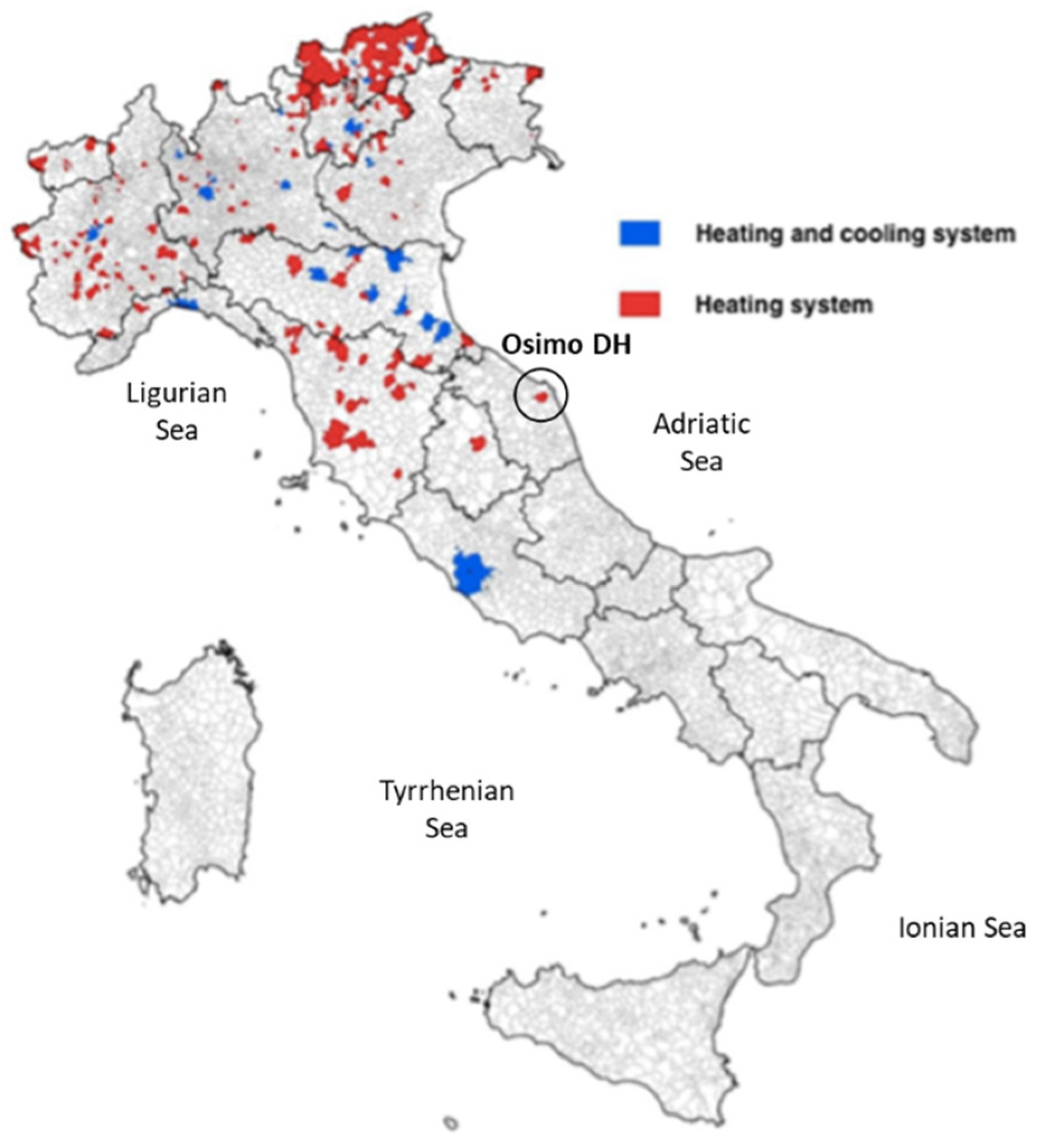
2. Case Study
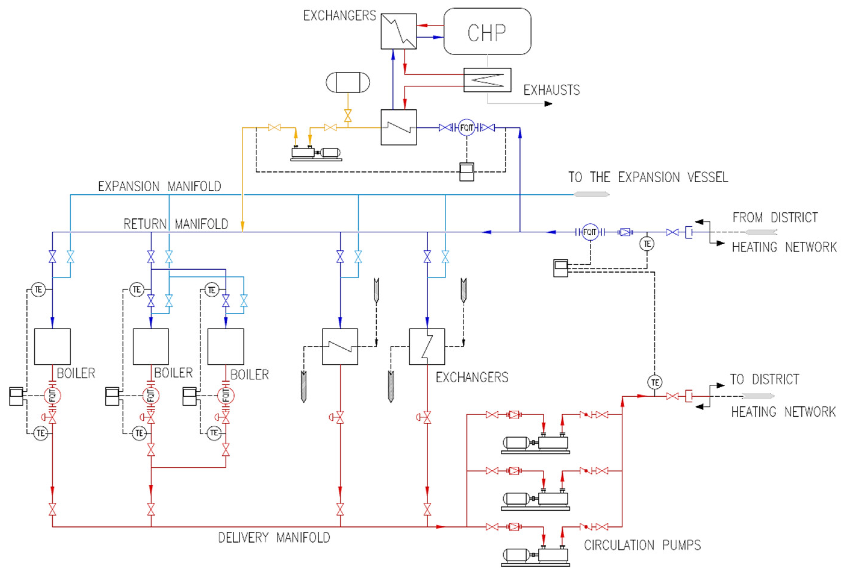
2.1. Thermal Power Plant
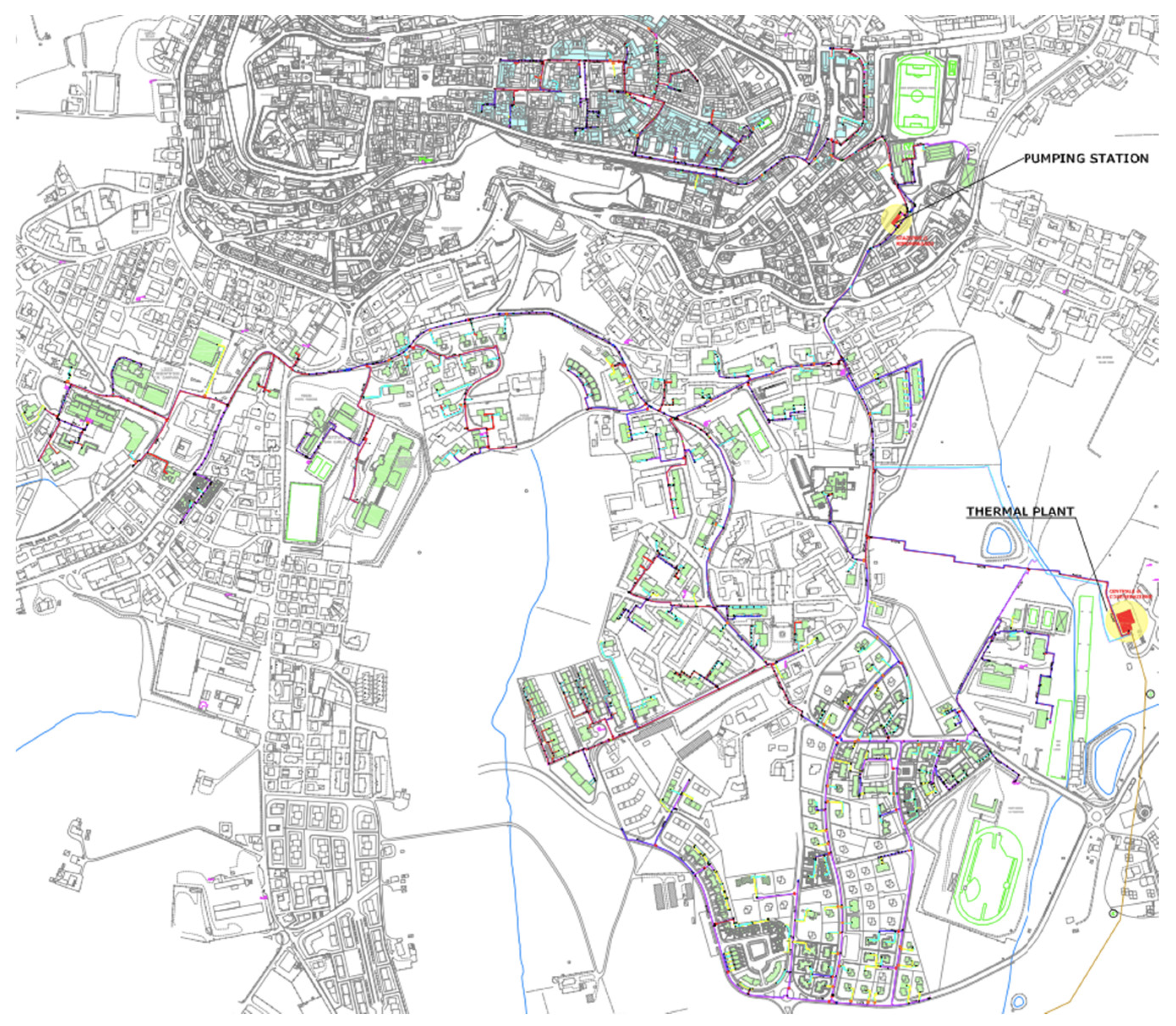
2.2. District Heating (DH) Network
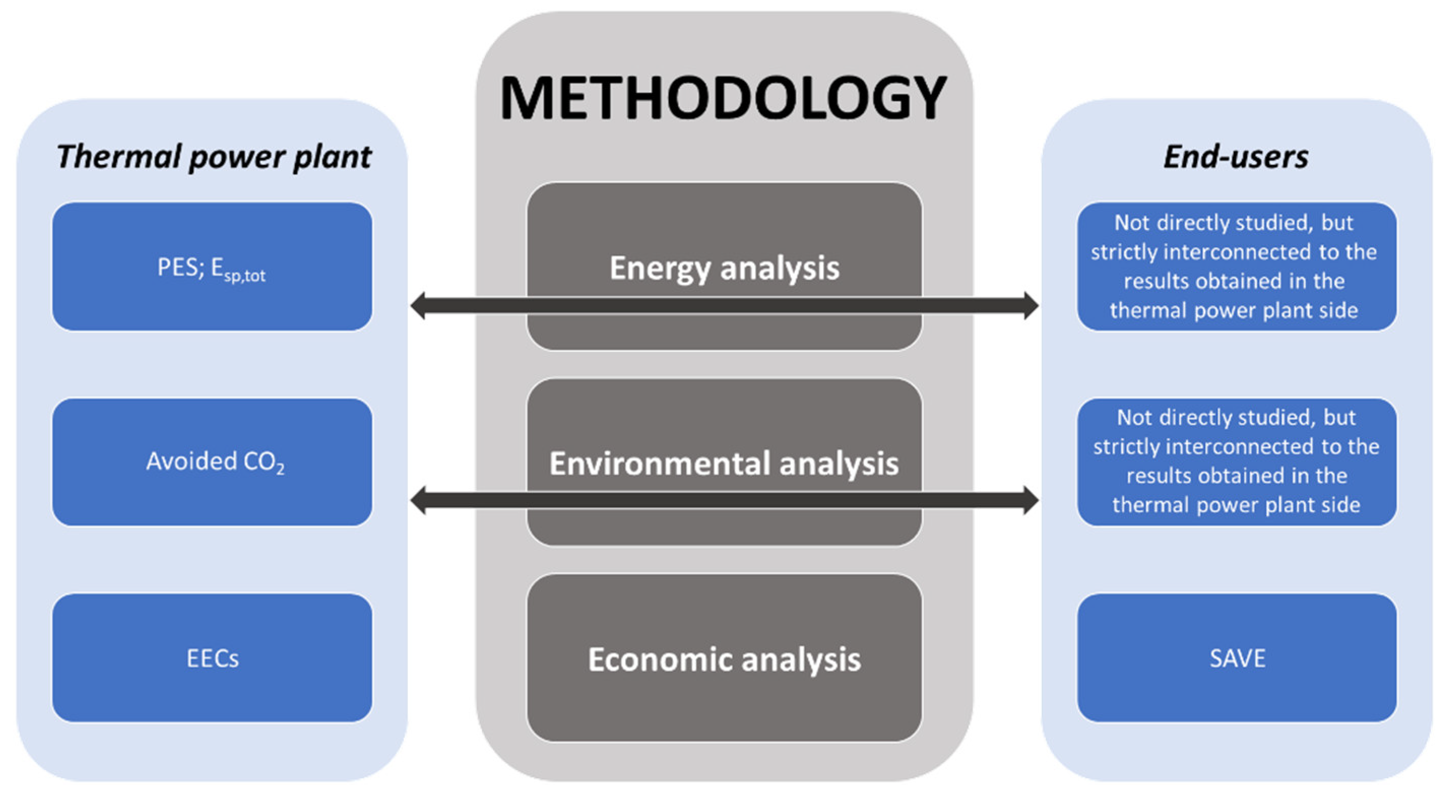
3. Methodology
3.1. Energy and Environmental Analysis
- -
- ηe,CHP is the electrical efficiency of the CHP unit, defined as the ratio between the yearly electricity produced by the cogeneration unit and the energy of the entire fuel supply used to produce both useful heat and electricity by the CHP unit;
- -
- ηe,ref is equal to 49.81% [33] and it is the reference efficiency value for the separate electricity production;
- -
- ηth,CHP is the thermal efficiency of the CHP unit, defined as the ratio between the yearly useful heat produced by the cogeneration unit and the energy of the entire fuel supply used to produce both useful heat and electricity by the CHP unit;
- -
- ηth,ref is equal to 92% [33] and it is the reference efficiency value for the separate heat production.
- -
- FcCO2 is the conversion factor, which is used to evaluate the avoided CO2 by knowing the energy that would have produced that amount of CO2, equal to 0.1936 kgCO2/kWh [34].
3.2. Economic Analysis
3.2.1. Thermal Power Plant Side
- -
- (RISP * 0086) is the saving, if positive, expressed in Tonnes of Oil Equivalent (TOE) and calculated according to Equation (10):
- -
- RISP is the primary energy savings, expressed in kWh, achieved by the CHP unit in the solar year in which access to the support scheme is requested;
- -
- ECHP is the electricity produced by the CHP unit in the same solar year expressed in MWh;
- -
- HCHP is the thermal energy produced by the CHP unit in the same solar year expressed in MWh;
- -
- FCHP is the energy consumed by the CHP unit in the same solar year expressed in MWh;
- -
- ηe,ref is the reference electric efficiency, which is equal to 0.53, and it must be adjusted according to the connection voltage, the amount of both consumed and supplied energies to the grid as well as the climatic zone;
- -
- ηth,ref is the reference thermal efficiency equal to 0.90;
- -
- K is a harmonized coefficient, equal to 1.386, and calculated as shown in [34].
3.2.2. End-Users’ Side
4. Results and Comments
4.1. Energy and Environmental Results
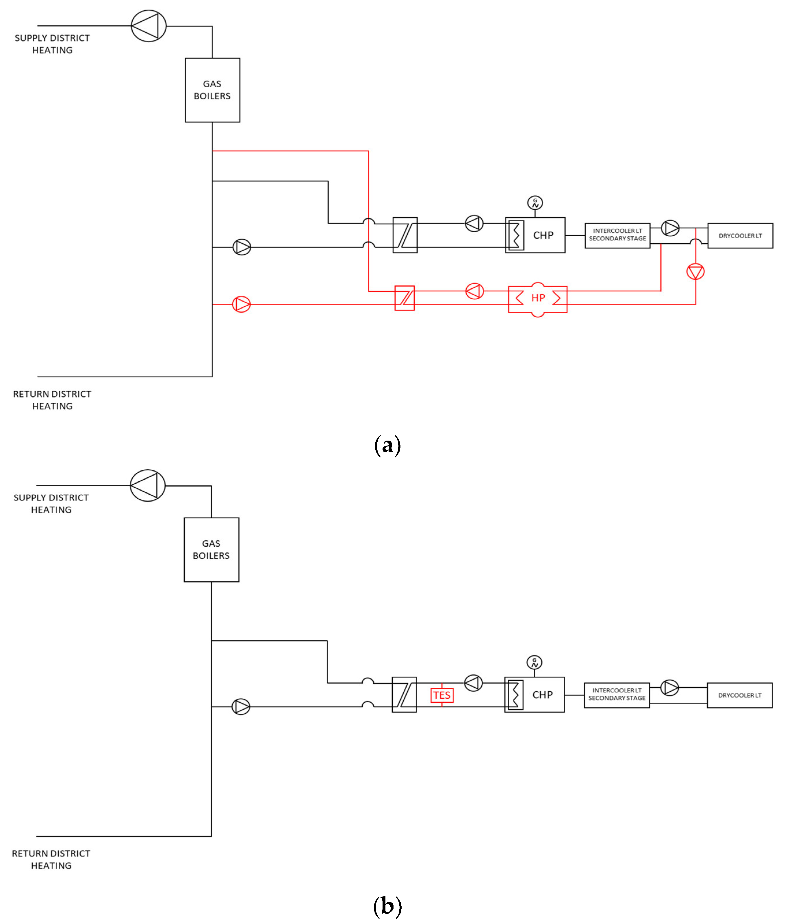
4.1.1. CHP + HP Configuration
4.1.2. CHP + TES Configuration
4.2. Economic Calculation
4.2.1. Thermal Power Plant Side
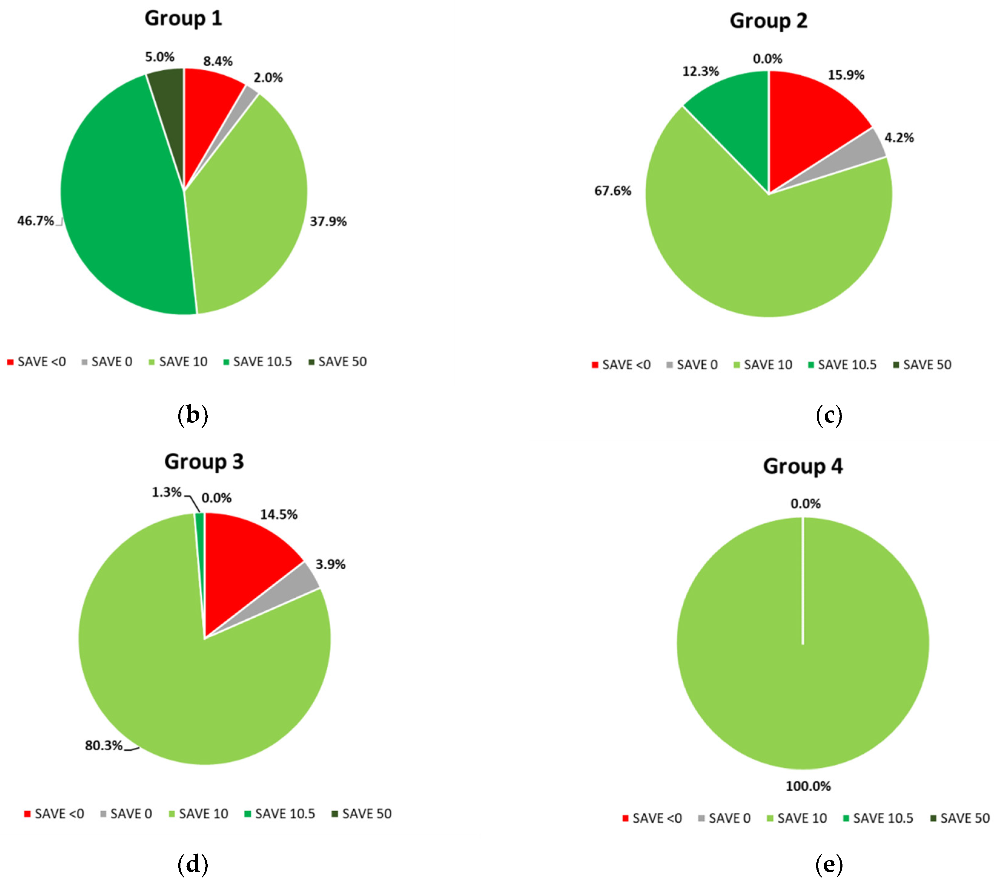
4.2.2. End-Users’ Side
5. Lessons Learned
6. Conclusions
Author Contributions
Funding
Acknowledgments
Conflicts of Interest
Abbreviations
| Nomenclature | |
| ∆Cost | difference between the overall yearly costs of end-users connected to the DH and those who have the IH |
| ∆Esp | delta specific energy |
| DHtot | overall yearly costs in 2019 for district heating |
| ECHP | electricity produced by the CHP unit in the same solar year |
| EEsp,CHP | specific electric energy of the CHP unit |
| Esp | specific energy |
| Esp,tot | total (thermal + electric) specific energy |
| Esth,el | thermal and electrical energy saving |
| FcCO2 | conversion factor to evaluate the avoided CO2, equal to 0.1936 kgCO2/kWh |
| FCHP | energy consumed by the CHP unit in the same solar year |
| HCHP | thermal energy produced by the CHP unit in the same solar year |
| IHtot | overall yearly costs in 2019 for individual heating |
| IHtot+extra costs | overall yearly costs in 2019 for individual heating + extra costs for maintenance, repairing, mandatory periodic boiler controls, cleaning, and check of the flue gases |
| K | harmonized coefficient, equal to 1.386 |
| LHVCH4 | Low Heating Value of methane gas |
| RISP | primary energy savings achieved by the CHP unit in the solar year |
| SAVE | the ratio between ∆Cost and DHtot, expressed in percentage |
| TEsp,boil | specific thermal energy of the boilers |
| TEsp,CHP | specific thermal energy of the CHP unit |
| ηe,CHP | electrical efficiency of the CHP unit |
| ηth,boil | thermal efficiency of the boilers |
| ηth,CHP | thermal efficiency of the CHP unit |
| ηe,ref | reference efficiency value for the separate electricity production |
| ηth,ref | reference efficiency value for the separate heat production |
| Acronyms | |
| CHP | Combined Heat & Power |
| DH | District Heating |
| DHC | District Heating and Cooling |
| EEC | Energy Efficiency Certificate |
| EU | European Union |
| EVs | Electric Vehicles |
| HP | Heat Pump |
| ICE | Internal Combustion Engine |
| iGDH | Generation of District Heating, where i = 1 to 5 represents the first to fifth generation |
| IH | Individual Heating |
| LHV | Low Heating Value |
| NG | Natural Gas |
| PBP | Payback Period |
| PES | Primary Energy Saving |
| PV | PhotoVoltaic |
| RES | Renewable Energy Sources |
| TES | Thermal Energy Storage |
| V2G | Vehicle-To-Grid |
References
- European Commission. Cause of Climate Change. Available online: https://ec.europa.eu/clima/change/causes_en (accessed on 15 October 2021).
- UN. Global Initiative for Resource Efficient Cities; United Nations Environment Programme: Paris, France, 2012; Available online: https://resourceefficientcities.org (accessed on 15 October 2021).
- European Commission. Clean Energy for All Europeans Package. Available online: https://ec.europa.eu/energy/topics/energy-strategy/clean-energy-all-europeans_en (accessed on 18 November 2020).
- Celiktas, M.; Kocar, G. From potential forecast to foresight of Turkey’s renewable energy with Delphi approach. Energy 2010, 35, 1973–1980. [Google Scholar] [CrossRef]
- Lund, H. Renewable energy strategies for sustainable development. Energy 2007, 32, 912–919. [Google Scholar] [CrossRef] [Green Version]
- Connolly, D.; Lund, H.; Mathiesen, B.V. Smart Energy Europe: The technical and economic impact of one potential 100% renewable energy scenario for the European Union. Renew. Sustain. Energy Rev. 2016, 60, 1634–1653. [Google Scholar] [CrossRef]
- Pilpola, S.; Arabzadeh, V.; Mikkola, J.; Lund, P.D. Analyzing National and Local Pathways to Carbon-Neutrality from Technology, Emissions, and Resilience Perspectives—Case of Finland. Energies 2019, 12, 949. [Google Scholar] [CrossRef] [Green Version]
- Lund, H.; Østergaard, P.A.; Chang, M.; Werner, S.; Svendsen, S.; Sorknæs, P.; Thorsen, J.E.; Hvelplund, F.; Mortensen, B.O.G.; Mathiesen, B.V.; et al. The status of 4th generation district heating: Research and results. Energy 2018, 164, 147–159. [Google Scholar] [CrossRef]
- Lund, H.; Werner, S.; Wiltshire, R.; Svendsen, S.; Thorsen, J.E.; Hvelplund, F.; Mathiesen, B.V. 4th Generation District Heating (4GDH): Integrating smart thermal grids into future sustainable energy systems. Energy 2014, 68, 1–11. [Google Scholar] [CrossRef]
- Lake, A.; Rezaie, B.; Beyerlein, S. Review of district heating and cooling systems for a sustainable future. Renew. Sustain. Energy Rev. 2017, 67, 417–425. [Google Scholar] [CrossRef]
- Rezaie, B.; Rosen, M.A. District heating and cooling: Review of technology and potential enhancements. Appl. Energy 2012, 93, 2–10. [Google Scholar] [CrossRef]
- Živić, M.; Galović, A.; Avsec, J.; Barac, A. Application of Gas Condensing Boilers in Domestic Heating. Teh. Vjesn. 2019, 26, 681–685. [Google Scholar] [CrossRef]
- Lund, H.; Østergaard, P.A.; Nielsen, T.B.; Werner, S.; Thorsen, J.E.; Gudmundsson, O.; Arabkoohsar, A.; Mathiesen, B.V. Perspectives on fourth and fifth generation district heating. Energy 2021, 227, 120520. [Google Scholar] [CrossRef]
- Lund, H.; Thellufsen, J.Z.; Aggerholm, S.; Wittchen, K.B.; Nielsen, S.; Mathiesen, B.V.; Möller, B. Heat Saving Strategies in Sustainable Smart Energy Systems. Int. J. Sustain. Energy Plan. Manag. 2015, 4, 3–16. [Google Scholar] [CrossRef]
- Sorknæs, P.; Østergaard, P.A.; Thellufsen, J.Z.; Lund, H.; Nielsen, S.; Djørup, S.; Sperling, K. The benefits of 4th generation district heating in a 100% renewable energy system. Appl. Energy 2020, 213, 119030. [Google Scholar] [CrossRef]
- Thellufsen, J.Z.; Lund, H.; Sorknæs, P.; Østergaard, P.A.; Chang, M.; Drysdale, D.; Nielsena, S.; Djørupa, S.R.; Sperling, K. Smart energy cities in a 100% renewable energy context. Renew. Sustain. Energy Rev. 2019, 129, 109922. [Google Scholar] [CrossRef]
- Averfalk, H.; Werner, S. Economic benefits of fourth generation district heating. Energy 2020, 193, 116727. [Google Scholar] [CrossRef]
- Ljubenko, A.; Poredoš, A.; Morosuk, T.; Tsatsaronis, G. Performance Analysis of a District Heating System. Energies 2013, 6, 1298–1313. [Google Scholar] [CrossRef]
- Domingo, A.M.M.; Rey-Hernández, J.M.; Alonso, J.F.S.J.; Crespo, R.M.; Martínez, F.J.R. Energy Efficiency Analysis Carried Out by Installing District Heating on a University Campus. A Case Study in Spain. Energies 2018, 11, 2826. [Google Scholar] [CrossRef] [Green Version]
- Neirotti, F.; Noussan, M.; Riverso, S.; Manganini, G. Analysis of Different Strategies for Lowering the Operation Temperature in Existing District Heating Networks. Energies 2019, 12, 321. [Google Scholar] [CrossRef] [Green Version]
- Spedaletti, S.; Rossi, M.; Comodi, G.; Salvi, D.; Renzi, M. Energy recovery in gravity adduction pipelines of a water supply system (WSS) for urban areas using Pumps-as-Turbines (PaTs). Sustain. Energy Technol. Assess. 2021, 45, 101040. [Google Scholar] [CrossRef]
- Comodi, G.; Caresana, F.; Salvi, D.; Pelagalli, L.; Lorenzetti, M. Local promotion of electric mobility in cities: Guidelines and real application case in Italy. Energy 2016, 95, 494–503. [Google Scholar] [CrossRef]
- Bartolini, A.; Comodi, G.; Salvi, D.; Østergaard, P.A. Renewables self-consumption potential in districts with high penetration of electric vehicles. Energy 2020, 213, 118653. [Google Scholar] [CrossRef]
- Comodi, G.; Lorenzetti, M.; Salvi, D.; Arteconi, A. Criticalities of district heating in Southern Europe: Lesson learned from a CHP-DH in Central Italy. Appl. Therm. Eng. 2017, 112, 649–659. [Google Scholar] [CrossRef]
- Kavian, S.; Hakkaki-Fard, A.; Mosleh, H.J. Energy performance and economic feasibility of hot spring-based district heating system—A case study. Energy 2020, 211, 118629. [Google Scholar] [CrossRef]
- Welsch, B.; Göllner-Völker, L.; Schulte, D.O.; Bär, K.; Sass, I.; Schebek, L. Environmental and economic assessment of borehole thermal energy storage in district heating systems. Appl. Energy 2018, 216, 73–90. [Google Scholar] [CrossRef]
- Arnaudo, M.; Giunta, F.; Dalgren, J.; Topel, M.; Sawalha, S.; Laumert, B. Heat recovery and power-to-heat in district heating networks—A techno-economic and environmental scenario analysis. Appl. Therm. Eng. 2021, 185, 116388. [Google Scholar] [CrossRef]
- Keçebaş, A. Energetic, exergetic, economic and environmental evaluations of geothermal district heating systems: An application. Energy Convers. Manag. 2013, 65, 546–556. [Google Scholar] [CrossRef]
- Yoon, T.; Ma, Y.; Rhodes, C. Individual Heating systems vs. District Heating systems: What will consumers pay for convenience? Energy Policy 2015, 86, 73–81. [Google Scholar] [CrossRef]
- Cao, B.; Zhu, Y.; Li, M.; Ouyang, Q. Individual and district heating: A comparison of residential heating modes with an analysis of adaptive thermal comfort. Energy Build. 2014, 78, 17–24. [Google Scholar] [CrossRef]
- Wang, Z. Heat pumps with district heating for the UK’s domestic heating: Individual versus district level. Energy Procedia 2018, 149, 354–362. [Google Scholar] [CrossRef]
- Rossi, M.; Cioccolanti, L.; Comodi, G.; Lorenzetti, M.; Salvi, D.; Arteconi, A. Thermal Energy Storage (TES) to increase the flexibility of cogeneration units in District Heating (DH) networks. In Proceedings of the ECOS 2021, the 34th International Conference on Efficiency, Cost, Optimization, Simulation and Environmental Impact of Energy Systems, Taormina, Sicily, Italy, 28 June–2 July 2021. [Google Scholar]
- European Commission. Commission Delegated Regulation (EU) 2015/2402 of 12 October 2015 Reviewing Harmonised Efficiency Reference Values for Separate Production of Electricity and Heat in Application of Directive 2012/27/EU of the European Parliament and of the Council and Repealing Commission Implementing Decision 2011/877/EU. Available online: https://eur-lex.europa.eu/eli/reg_del/2015/2402/oj (accessed on 15 November 2020).
- Agenzia Nazionale per le Nuove Tecnologie, L’energia e lo Sviluppo Economico Sostenibile (ENEA). Rapporto Energia e Ambiente 2002. Available online: http://old.enea.it/com/web/pubblicazioni/REA_02/analisi_02.pdf (accessed on 15 October 2021). (In Italian).
- Ministero dello Sviluppo Economico (MISE). Decreto Ministeriale 5 Settembre 2011—Regime di Sostegno per la Cogenerazione ad Alto Rendimento. Available online: https://www.mise.gov.it/index.php/it/89-normativa/decreti-ministeriali/2020499-decreto-ministeriale-5-settembre-2011-regime-di-sostegno-per-la-cogenerazione-ad-alto-rendimento (accessed on 15 October 2021). (In Italian)
- Astea S.p.A. Available online: https://www.asteaspa.it/wp-content/uploads/2019/10/Tariffe-Teleriscaldamento-2019.pdf (accessed on 15 October 2021).
- Autorità di Regolazione per Energia Reti e Ambiente (ARERA). Stato dei Servizi. 2019. Volume 1. Available online: https://www.arera.it/allegati/relaz_ann/20/RA20_volume1.pdf (accessed on 15 October 2021).
- Cadau, N.; De Lorenzi, A.; Gambarotta, A.; Morini, M.; Rossi, M. Development and Analysis of a Multi-Node Dynamic Model for the Simulation of Stratified Thermal Energy Storage. Energies 2019, 12, 4275. [Google Scholar] [CrossRef] [Green Version]
- Mugnini, A.; Polonara, F.; Arteconi, A. Energy flexibility curves to characterize the residential space cooling sector: The role of cooling technology and emission system. Energy Build. 2021, 253, 111335. [Google Scholar] [CrossRef]


| Magnitude [Unit of Measure] | Values |
|---|---|
| CHP unit rated electric power [MW] | 1.2 |
| CHP unit rated thermal power [MW] | 1.3 |
| Boilers rated thermal power [MW] | 13.4 |
| ηth,CHP [-] | 0.42 |
| ηe,CHP [-] | 0.41 |
| ηth,boil [-] | 0.962 |
| Month | 1 | 2 | 3 | 4 | 5 | 6 | 7 | 8 | 9 | 10 | 11 | 12 |
|---|---|---|---|---|---|---|---|---|---|---|---|---|
| Heat losses [MWh] | 643.7 | 575.8 | 564.6 | 497.0 | 487.6 | 406.4 | 353.0 | 345.1 | 369.2 | 432.5 | 496.2 | 563.7 |
| Incidence of the heat losses [%] | 16.6 | 20.2 | 27.0 | 34.0 | 39.8 | 60.6 | 61.3 | 62.1 | 56.3 | 50.2 | 28.8 | 20.5 |
| Parameters | EEC Calculation (Italian Legislation [35]) | PES Calculation (EU Legislation [33]) |
|---|---|---|
| ηe,ref (a) [-] | 0.46 | 0.53 |
| Correction factor 1: climatic zone (b) [-] | 0.00369 | 0.00369 |
| Correction factor 2: off-site (c) [-] | 0.945 1 | 0.935 2 |
| Correction factor 3: on-site (d) [-] | 0.925 1 | 0.914 2 |
| ηe,tot = (a + b)*(c * EEdel 3 + d * EEself-cons 3) [-] | 0.4374 | 0.4981 |
| ηth,ref [-] | 0.90 | 0.92 |
| Parameters | Values |
|---|---|
| Average cost of maintenance, periodic boiler control, cleaning, and check of the flue gases [€/year] | 100 |
| Average cost for repairing [€/year] | 50 |
| Average cost of electricity to switch-on the boiler [€/year] | 20 |
| Total [€/year] | 170 |
| Month | CHP NG Consumption [Sm3] | Boiler NG Consumption [Sm3] | CHP TE Production [MWh] | Boiler TE Production [MWh] | DH Load [MWh] | CHP Unit EE Production [MWh] | CHP Unit EE Delivered [MWh] |
|---|---|---|---|---|---|---|---|
| 1 | 230,266 | 342,387 | 915.0 | 2971.7 | 3243.0 | 878.4 | 804.21 |
| 2 | 207,910 | 230,301 | 822.8 | 2025.5 | 2272.5 | 793.5 | 733.83 |
| 3 | 211,114 | 143,278 | 832.7 | 1254.7 | 1522.8 | 804.9 | 753.00 |
| 4 | 187,692 | 76,050 | 733.8 | 725.8 | 962.6 | 713.9 | 661.53 |
| 5 | 108,686 | 86,382 | 424.8 | 800.5 | 737.7 | 411.6 | 376.85 |
| 6 | 43,548 | 53,861 | 165.7 | 505.2 | 264.5 | 162.5 | 146.44 |
| 7 | 0 | 65,468 | 0.0 | 576.2 | 223.2 | 0.0 | 0.0 |
| 8 | 0 | 62,047 | 0.0 | 556.0 | 210.9 | 0.0 | 0.0 |
| 9 | 27,280 | 60,587 | 101.3 | 554.3 | 286.4 | 102.4 | 92.87 |
| 10 | 120,848 | 39,490 | 460.8 | 400.8 | 429.1 | 458.0 | 420.26 |
| 11 | 185,260 | 100,635 | 749.2 | 971.2 | 1224.2 | 708.5 | 647.42 |
| 12 | 231,267 | 196,227 | 937.0 | 1818.0 | 2191.3 | 887.5 | 798.47 |
| Total | 1,553,871 | 1,456,713 | 6143.1 | 13,159.9 | 13,568.2 | 5921.2 | 5434.9 |
| Month | PES [%] | TEsp,CHP [kWh/Sm3] | TEsp,boil [kWh/Sm3] | EEsp,CHP [kWh/Sm3] | Esp,tot [kWh/Sm3] | ∆Esp [kWh/Sm3] | Eth,el [kWh] | Avoided CO2 [Tonnes] |
|---|---|---|---|---|---|---|---|---|
| 1 | 21.5 | 3.32 | 7.24 | 3.81 | 14.37 | 4.97 | 1,906,550 | 369 |
| 2 | 21.4 | 3.16 | 7.02 | 3.82 | 13.99 | 4.59 | 1,233,595 | 239 |
| 3 | 21.3 | 2.88 | 6.39 | 3.81 | 13.08 | 3.68 | 662,448 | 128 |
| 4 | 20.9 | 2.58 | 6.29 | 3.80 | 12.68 | 3.28 | 372,941 | 72 |
| 5 | 20.7 | 2.35 | 5.58 | 3.79 | 11.72 | 2.32 | 202,329 | 39 |
| 6 | 19.2 | 1.50 | 3.70 | 3.73 | 8.93 | −0.47 | - | - |
| 7 | 0.0 | - | 3.41 | - | 3.41 | −5.99 | - | - |
| 8 | 0.0 | - | 3.40 | - | 3.40 | −6.00 | - | - |
| 9 | 18.8 | 1.62 | 4.00 | 3.75 | 9.37 | −0.02 | - | - |
| 10 | 20.0 | 1.90 | 5.05 | 3.79 | 10.74 | 1.34 | 68,168 | 13 |
| 11 | 22.2 | 2.88 | 6.87 | 3.82 | 13.57 | 4.17 | 603,501 | 117 |
| 12 | 22.4 | 3.22 | 7.37 | 3.84 | 14.43 | 5.03 | 1,302,964 | 252 |
| Average | 21.3 | 2.78 | 6.35 | 3.81 | 12.94 | 3.54 | 5,678,900 | 1099 |
| CHP + TES Configuration | |||||||||||
|---|---|---|---|---|---|---|---|---|---|---|---|
| Month | ηth,CHP+TES [%] | ηe,CHP+TES [%] | ηth+e,CHP+TES [%] | PES [%] | 1 TEsp,CHP+TES [kWh/Sm3] | 1 TEsp,boil [kWh/Sm3] | 1 EEsp,CHP+TES [kWh/Sm3] | 1 Esp,tot [kWh/Sm3] | 1 ΔEsp [kWh/Sm3] | Eth,el [kWh] | Avoided CO2 [tonnes] |
| 1 | 42.3 | 40.6 | 82.9 | 21.5 | 3.32 | 7.24 | 3.81 | 14.37 | 4.97 | 1,906,550 | 369 |
| 2 | 42.1 | 40.6 | 82.7 | 21.4 | 3.16 | 7.02 | 3.82 | 13.99 | 4.59 | 1,233,595 | 239 |
| 3 | 42.0 | 40.6 | 82.6 | 21.3 | 2.88 | 6.39 | 3.81 | 13.08 | 3.68 | 662,448 | 128 |
| 4 | 41.6 | 40.5 | 82.1 | 20.9 | 2.58 | 6.29 | 3.80 | 12.68 | 3.28 | 372,941 | 72 |
| 5 | 42.8 | 41.2 | 84.0 | 22.6 | 2.42 | 2.11 | 3.87 | 8.41 | −0.99 | - | - |
| 6 | 40.9 | 39.4 | 80.3 | 19.1 | 1.52 | 0.41 | 3.70 | 5.63 | −3.77 | - | - |
| 7 | 42.3 | 40.7 | 83.0 | 21.7 | 1.54 | - | 3.83 | 5.37 | −4.03 | - | - |
| 8 | 42.3 | 40.8 | 83.2 | 21.8 | 1.51 | - | 3.84 | 5.35 | −4.05 | - | - |
| 9 | 42.6 | 41.0 | 83.6 | 22.3 | 1.75 | 0.75 | 3.86 | 6.36 | −3.04 | - | - |
| 10 | 42.8 | 41.2 | 83.9 | 22.6 | 2.00 | 2.80 | 3.87 | 8.67 | −0.73 | - | - |
| 11 | 43.0 | 40.7 | 83.7 | 22.2 | 2.88 | 6.87 | 3.82 | 13.57 | 4.17 | 603,501 | 117 |
| 12 | 43.1 | 40.8 | 83.9 | 22.4 | 3.22 | 7.37 | 3.84 | 14.43 | 5.03 | 1,302,964 | 252 |
| Average (5–10) | 42.3 | 40.8 | 83.1 | 21.8 | 1.83 | 1.93 | 3.83 | 7.60 | −1.80 | - | - |
| Average (yearly) | 42.3 | 40.7 | 83.0 | 21.7 | 3.17 | 6.95 | 10.12 | 13.94 | 4.54 | 8,217,808 | 1591 |
| Month | 1 | 2 | 3 | 4 | 5 | 6 | 7 | 8 | 9 | 10 | 11 | 12 | Total |
|---|---|---|---|---|---|---|---|---|---|---|---|---|---|
| RISP [MWh] | 1036.0 | 931.5 | 942.5 | 830.8 | 481.1 | 187.7 | - | - | 114.8 | 522.0 | 848.1 | 1061.0 | 6955.6 |
| Italian EECs [-] | 123 | 111 | 112 | 99 | 57 | 23 | - | - | 14 | 63 | 101 | 126 | 829 |
| Income [€] | 30,845 | 27,719 | 28,028 | 24,736 | 14,315 | 5682 | - | - | 3455 | 15,616 | 25,230 | 31,566 | 207,222 |
Publisher’s Note: MDPI stays neutral with regard to jurisdictional claims in published maps and institutional affiliations. |
© 2021 by the authors. Licensee MDPI, Basel, Switzerland. This article is an open access article distributed under the terms and conditions of the Creative Commons Attribution (CC BY) license (https://creativecommons.org/licenses/by/4.0/).
Share and Cite
Corradi, E.; Rossi, M.; Mugnini, A.; Nadeem, A.; Comodi, G.; Arteconi, A.; Salvi, D. Energy, Environmental, and Economic Analyses of a District Heating (DH) Network from Both Thermal Plant and End-Users’ Prospective: An Italian Case Study. Energies 2021, 14, 7783. https://doi.org/10.3390/en14227783
Corradi E, Rossi M, Mugnini A, Nadeem A, Comodi G, Arteconi A, Salvi D. Energy, Environmental, and Economic Analyses of a District Heating (DH) Network from Both Thermal Plant and End-Users’ Prospective: An Italian Case Study. Energies. 2021; 14(22):7783. https://doi.org/10.3390/en14227783
Chicago/Turabian StyleCorradi, Erica, Mosè Rossi, Alice Mugnini, Anam Nadeem, Gabriele Comodi, Alessia Arteconi, and Danilo Salvi. 2021. "Energy, Environmental, and Economic Analyses of a District Heating (DH) Network from Both Thermal Plant and End-Users’ Prospective: An Italian Case Study" Energies 14, no. 22: 7783. https://doi.org/10.3390/en14227783
APA StyleCorradi, E., Rossi, M., Mugnini, A., Nadeem, A., Comodi, G., Arteconi, A., & Salvi, D. (2021). Energy, Environmental, and Economic Analyses of a District Heating (DH) Network from Both Thermal Plant and End-Users’ Prospective: An Italian Case Study. Energies, 14(22), 7783. https://doi.org/10.3390/en14227783