Review

Analysis of Natural Gas Consumption Interdependence for Polish Industrial Consumers on the Basis of an Econometric Model

1
AGH Doctoral School, AGH University of Science and Technology, Mickiewicza 30 Av., 30-059 Krakow, Poland
2
Gas Engineering Department, Drilling, Oil and Gas Faculty, AGH University of Science and Technology, Mickiewicza 30 Av., 30-059 Krakow, Poland
*
Author to whom correspondence should be addressed.
Energies 2021, 14(22), 7649; https://doi.org/10.3390/en14227649
Submission received: 20 October 2021 / Revised: 8 November 2021 / Accepted: 13 November 2021 / Published: 16 November 2021
(This article belongs to the Topic Exergy Analysis and Its Applications)

Abstract

:
The transmission of natural gas is a key element of the Polish energy system. The published data of the Polish distribution system operators and the transmission system operator on the volume of gaseous fuel transmitted indicate a growing trend in the consumption of energy produced from natural gas. In connection with the energy transformation, switching energy generation sources from hard coal to natural gas in Poland, it is important for transmission operators to know the future demand for gaseous fuel. The aim of the article is to attempt to develop an econometric model related to the consumption of gaseous fuel by Polish entrepreneurs. The knowledge therein may be useful for making business decisions related to the possible expansion of the transmission system, and thus investing financial resources for this purpose. This knowledge will also provide quantitative information related to the interest in gaseous fuel among industrial consumers and the analysis of the trend of natural gas consumption in Poland in the aspect of energy transition. The intention of the publication was to determine the macroeconomic indicators that strongly affect natural gas consumption by the Polish industry and the quantitative growth of consumption depending on changes in these indicators. The results showed that the highest correlation of the growth of natural gas consumption is related to the production of chemistry, the chemical industry, and the power industry.

1. Introduction

The motivation of the article was to present the cause–effect analysis of the influence of external factors on the consumption of natural gas by the Polish industry. The research was based on the most frequently used estimation method in economics, i.e., the least squares method. It is shown that by estimating the unknown model parameters with this method, it is possible to obtain estimates for which the model best provides a description of the observed data. In recent years there has been a lack of research on the proposed topic; the results of the analysis may be useful to illustrate the essence of this natural gas in the energy transition. The transmission of natural gas is one of the main components of the country’s energy system [1]. The published data of the operators of the national distribution system and the transmission system, regarding the volume of gaseous fuel transmitted, testify to an upward trend in the consumption of energy produced from natural gas [2]. The basic task of the operators transmitting natural gas to the final consumers is its safe delivery and the guarantee of the continuity of supplies without any disturbances, and ensuring the continuity of the supplies has a decisive impact on maintaining the energy security and maintaining stability of the economy based on natural gas sources [3].
In connection with energy transformation, the switch of energy production sources from hard coal to natural gas, it is crucial for transmission operators to predict the future demand for gaseous fuel [4]. Knowledge of future phenomena related to the consumption of gaseous fuel provides business decisions related to the possible expansion of the transmission system and thus in investing financial resources for this purpose. The prediction also provides quantitative information related to the interest in gaseous fuel among industrial consumers and checking the trend of natural gas consumption in Poland in the aspect of energy transition.
It should be emphasized in this context that the current energy transformation is significantly influenced by the European Union’s climate and energy policy, including its long-term vision of achieving climate neutrality by 2050. In reference to the European Union’s climate and energy policy, Poland has developed its energy policy until 2040. PEP2040 contributes to the implementation of the Paris Agreement concluded in December 2015 during the 21st Conference of the Parties to the United Nations Framework Convention on Climate Change (COP21) [5]. A critical element of PEP 2040 is natural gas, which is expected to be the bridge fuel in the energy transition. The national resource potential offers the possibility of independently covering the demand for coal and biomass, but most of the demand for natural gas has to be covered by imports.
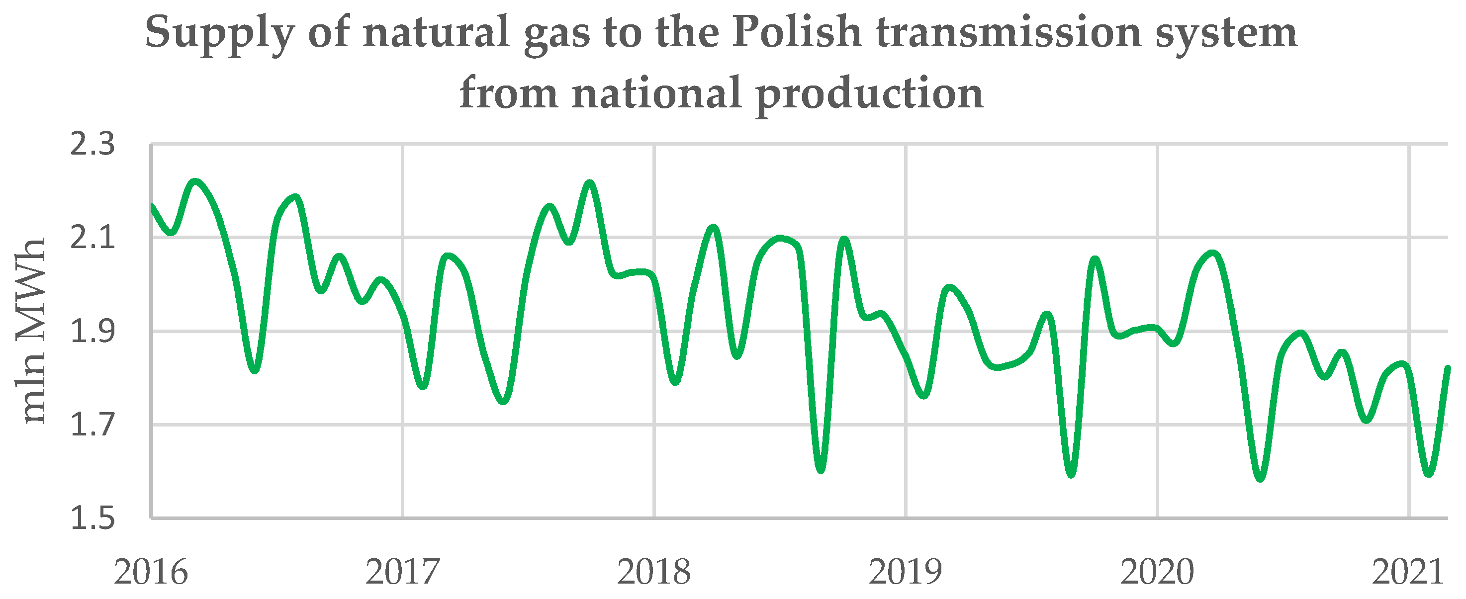
Despite the increase in the number of recognized hydrocarbon fields (Table 1) from year to year, the volume of natural gas from national production transmitted to the national transmission system is decreasing (Figure 1). This confirms that diversification of supplies from various sources guarantees persistence security. The fossil energy resources (coal, oil, and natural gas) currently have no substitutes to match the required energy demand. Poland has no chance to be self-sufficient in covering the country’s demand for oil and natural gas [6]. Due to this fact, it is important to diversify the supply routes [7]. An important aspect of ensuring energy production in Poland is still the production of electricity from coal.
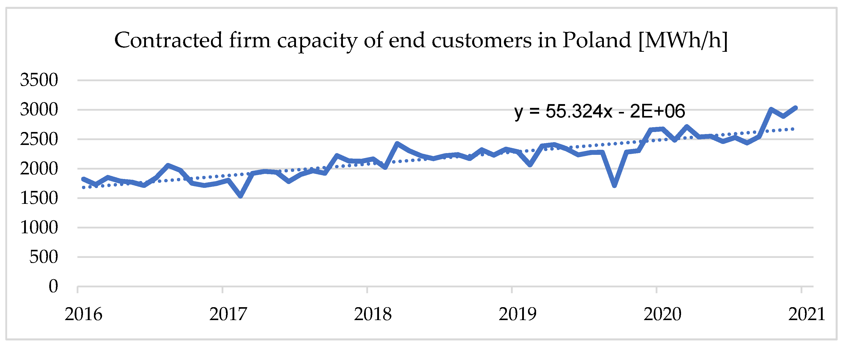
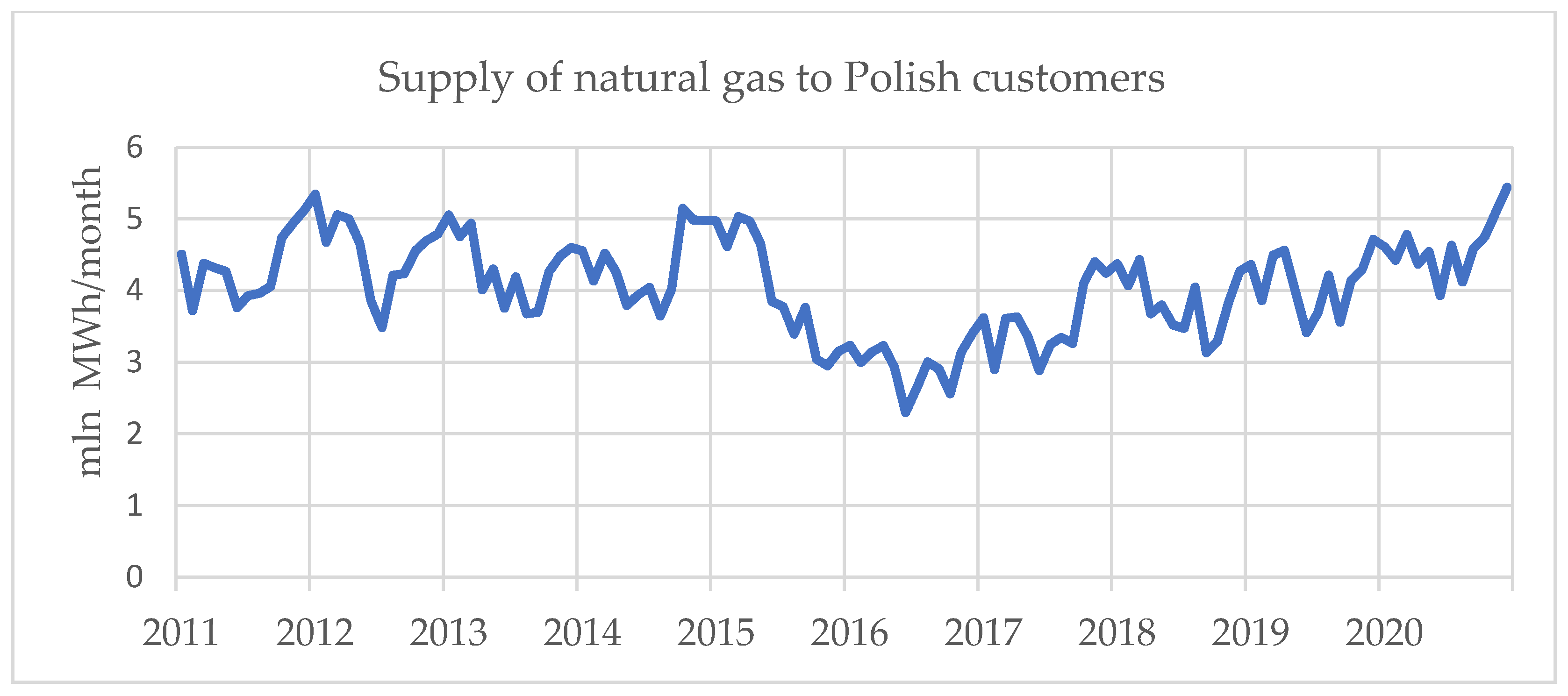
Many factors may influence the consumption of natural gas by final consumers (industrial consumers, households) [8]. It is important to note that there is growing interest in gaseous fuel in Poland (Figure 2) Based on the literature on the subject, several potential factors can influence the consumption of natural gas in Poland and can be identified [9,10]. These are described in the following section. It is necessary to mention that the influence of the coronavirus pandemic on the volumes of transmitted natural gas volumes has also been noticed recently [11]. Consequently, there is no attempt to build a model for the years 2020–2021, as they are affected by the deformation of the time series related to the supply of gaseous fuels.
This article can also fill the research gap in the field of the possibility of using econometric models to describe the consumption of natural gas in Poland by industrial consumers, in a country aspiring to create a gas hub in the future and switching from coal-based to gas-based power generation. Furthermore, the Polish transmission network is currently being extended, with interconnections with Lithuania, Slovakia, the Czech Republic, and the North-South Gas Corridor being developed. It should be added that an analysis of recent publications has not revealed any material concerning an attempt to analyze the interdependence of natural gas consumption by Polish industry; moreover, such publications are practically nonexistent. Of course, there are scientific articles that present forecasts, using mechanical forecasting techniques, without a thorough analysis of external factors that could affect the consumption of natural gas. The article analyzes the possibility of using a few dozen macroeconomic indicators, which may describe the phenomenon under study. Finally, 12 factors were selected for the article. Preliminary analysis showed that they have the greatest influence on consumption. The article presents their potential and the possibility of using them in the final econometric model. The contribution of the paper is the collection of macroeconomic indicators describing the current prevailing reality on the Polish natural gas market together with their interpretation. In particular, attention was paid to the most important determinants affecting natural gas consumption by the Polish economy, so that the continuity of supply is maintained and the perspective of new connections of customers with the gas network is created. This knowledge may be useful for gas operators and energy companies.

Review of the Literature

One of the recent scientific publications that attempted to analyze the interdependence of energy consumption by end users is an article by Muglabeh et al., 2021 [12]. The results showed that energy consumption significantly affected economic growth and that there is a common causal relationship. Radmeher et al. 2021 show by means of phenomenon interdependence analysis, an interesting relationship between economic growth and carbon emissions and between economic growth and renewable energy consumption is bidirectional [13]. Abbasi 2021, also using econometric modeling, indicated that the industrial sector is a key factor in overall energy demand, closely related to the economy. Empirical analysis shows that these factors are cointegrated. While a 1% increase in electricity consumption causes the price of electricity to fall by 0.19%, if the GDP increases by 1%, the price of electricity falls by 0.16% [14]. Furthermore, Gerhson et al. 2021 indicated that fossil fuels are significant drivers of real GDP or economic growth for Nigeria [15].
An interesting publication in the area under review was the “Macroeconomic Short-Term High-Precision Combination Forecasting Algorithm” paper, which indicated that to calculate the potential growth rate, the three factors of potential total factor productivity, labor, and capital stock must be estimated and then the existing growth accounting model must be used to calculate the potential output [15].
Econometric modeling can be used to describe the energy balancing structure. In one publication, the authors studied the relationship between electricity consumption and economic reform. A 1% increase in economic output increases electricity consumption by 0.22% (income elasticity of electricity demand) [16].
Using econometric modeling, Ghosh et al. 2021 developed a model that optimizes the retail input, the wholesale price demanded by the producer, the environmental performance of the product and the selling price charged by retailers [17].
The coefficients in the econometric model can be interpreted as long-term elasticities, as the variables form a natural logarithm. Thus, CO2 emissions increase with the level of production and consumption of fossil fuel-based energy. For example, a 3% increase in economic activity increases emissions by 1.27%, while a 3% increase in fossil fuel energy consumption will increase total emissions by 1.69%, assuming other factors remain constant. Research on data on the Mexican economy found evidence of a bidirectional causal relationship between energy and production, indicating that the two variables form a complementary process, that is, an increase in GDP is accompanied by an increase in energy demand [18].
The causal analysis [19] based on the empirical model indicated that natural gas consumption in Indonesia is a boost to the welfare of the country. The other authors have the same observation that, based on an econometric model, confirms the hypothesis of natural gas consumption induced by economic growth [20]. The authors recommend that policy makers intensify efforts to increase the accumulation of physical and human capital to offset industrialization, which will result in an increase in natural gas consumption in Malaysia. The next article indicated in an econometric model that an increase in natural gas consumption in the Mediterranean region leads to industrial growth [21]. Makala [22] made an attempt to analyze the relationship between industrial growth and natural gas consumption, his research focusing on finding a relationship between natural gas consumption and economic growth in Tanzania. The other notable publication is the analysis of the natural gas market in Germany [23], in which the authors analyze the factors in the construction of a statistical model of natural gas consumption. It is indicated that the main factors are population and outdoor temperature. Based on linear regression analysis, the authors indicated the relationship of explanatory variables such as population and temperature. Such analyzes were based on econometric models made from the perspective of domestic consumption. However, the construction of an econometric model can be applied in various contexts to the impact of natural gas consumption in buildings, with regard to homes and offices. Therefore, the method can be used successfully from the point of view of the local consumer. The linear regression method can also be used in hybrid combination with other methods such as artificial neural networks, random forests, vector machines [24]. The building of econometric models can also be successfully used in the perspective of renewable energy deposits. A successful application of the model used for hydroelectric plants is a promising approach [25]. The authors argue that these models can estimate the construction time of hydroelectric plants, which will help support environmental protection projects. The literature review concluded that in the research paper, the authors of building an econometric model using the method of correlation analysis of natural gas consumption indicate that economic development stimulates natural gas consumption.

2. Material and Methods

The objective of the paper is to determine the nature and type of cause-and-effect relationships for the consumption of natural gas by Polish end consumers. Econometric model building (classical least squares method) can be used for this purpose. In the classical least squares method, the assumptions must be considered, among all: the estimated econometric model is linear with respect to the parameters, and the explanatory variables xi are nonrandom quantities with fixed elements.
Consequently, it is reasonable to make an attempt to estimate a model that characterizes the dependence of gaseous fuel consumption on selected factors.
In general, the analytical form of such a model can be written as [26]:
Y = α 0 + α 1 x 1 + α 2 x 2 + + α n x n + ε
The purpose of the model was to present the relationship between the explained variable Y and the explanatory variables xn. It was assumed in the paper that the consumption of natural gas by consumers constituted the explanatory (dependent) variable Y, and the potential explanatory (independent) variables, potentially characterizing the factors influencing the value of natural gas consumption, would be marked as xn. α0,…, αn-parameters to be determined. In the following section, the basic sequence of econometric modeling procedures has been presented. Figure 3 illustrates the procedure for the construction of the econometric model.
The analysis covered the period January 2011 to December 2015, because in this period the end users observed stable deliveries, thus providing the basis for the construction of the econometric model (Figure 4). In addition, Figure 5, in contrast, presents a time series of potential variables during the period under study. The graph is only intended to show the nature of the run of observations.

Principal Characteristics of the Variables

The main part of the construction of the econometric model using the least-squares method is the specification of the variables, including data collection. The selection of explanatory variables from the originally adopted set was preceded by checking the existence of significant relationships between potential independent variables and the dependent variable. The hypotheses of stochastic independence for the examined characteristics were verified using Pearson’s chi-square independence test. The literature review suggested a relationship between natural gas consumption and GDP [27]. A study of a comprehensive review of macroeconomic indicators published by the Central Statistical Office was conducted in a monthly class. Analysis of the literature indicated that the three main influencing factors with the highest correlation with natural gas demand in the structure of energy consumption, GDP and urbanization rate, successively [28]. The published results for Indonesia as a country rich in its natural resources are to be one of the countries in the world that plays an active role in increasing international trade flows, it has been shown that in the short term, all variables such as domestic consumption, exchange rate, natural gas prices, and GDP per capita have a significant impact on the volume of natural gas exports and imports [29]. Additionally, other studies indicate factors such as total population, gross domestic products, urbanization rate, industrial structure, energy consumption structure, and carbon dioxide emission to be colinear with natural gas consumption. In addition, it points out the strongly correlated relationship between natural gas consumption and outside air temperature. Natural gas demand generally increases in the coldest months and decreases in the warmest months, with a slight increase in the summer to meet the demand for electric generators [30].
The data on macroeconomic indicators were all taken from EUROSTAT.

3. Experimental

3.1. Propose Optimal Macroeconomic Indicators

The first is the compilation of a selection of potential explanatory variables based on knowledge about the phenomenon under analysis. These variables are obtained by knowledge of the theory of the given field of knowledge. The criterion for selection should be substantive knowledge of the studied phenomena. Factors should be selected (explanatory variables) that have a significant impact on the formation of the phenomenon researched. The variables collected in this manner will be called the set of potential explanatory variables. The most important formal and statistical criteria in the methods of variable selection are: the variables should be characterized by high variability, ensure maximum correlation of the explanatory variable with the explanatory variables. The explanatory variables should not be significantly correlated among themselves. The maximum degree of fit of the model to the actual economic relations should be sought, which is expressed in the maximization of the coefficient of determination R2, which is done in the article in the following section. Subsequently, a reduction of the set of explanatory variables is made, guided by statistical criteria. The article relies on the graph method, the study of correlation significance, and information capacity.
The first step in building the econometric model was to study the specification of potential macroeconomic indicators that affect the consumption by gaseous fuel of industrial consumers [31]. The selection of explanatory variables for a causal model should be based on the theory of the relevant field of knowledge, the experience of the principal and statistics, and trial and error methods (intuitive). Based on a general analysis of the macroeconomic indicators made available by EUROSTAT, the study selected the most potential ones (Table 2).
After analyzing the proposed macroeconomic indicators, in terms of the construction of a time series that can be used to build an econometric model (Table 3), it was decided to select (highest p-values):
Table 4 determined the essential statistical calculations needed to develop the model, using GRETL software [32]. An open source statistical package used mainly in econometrics.
The above results are not discussed because non-stationarity in individual macroeconomic indicators had to be removed. The results are discussed in detail in further detail in the article.

3.2. Checking the Seasonality and Removal of Nonstationarity

The following fundamental step requires checking the seasonality of the time series of the variables (Table 5). The variables can be used in the model, but an issue is the risk of apparent regression. This regression occurs if the analyst considers the variables in the model and ignores the fact that they are stationary.
Non-stationarity is eliminated in order for the data to be distributed normally and to achieve stationarity. As a result of the analysis, it was found that trends occur in the time series of variables X3, X4, X6, X8, X10. These series have the feature of trend-stationarity. The basic element in building an econometric model is to remove non-stationarity [33]. For the indicated variables, trend stationarity was removed by the differentiation method (Table 6).
The above results are reasonably satisfactory (Table 7), but the objective was to achieve even better results, striving to obtain Stat. Durbina-Watsona ~2,0 [34].
The best results intended for the assumptions were obtained after removing the variables: X7, X8, X12 (Table 8):
The p-value for the F-test was 5.33 × 10⁻⁸ (Table 9) which is a quite satisfactory result, the proposed arrangement of variables has explanatory power [35]. The coefficient of determination of R-square was 0.87, and this is sufficient to provide an analysis of the relationship. The information criteria of Akaike, Hannan–Quinn, and the Bayes–Schwarz criterion are close to each other, satisfactory result [36]. Furthermore, the values of the Durbin-Warson statistic are greater than the coefficient of determination R-square, a satisfactory result [37]. Another important information is the result obtained from the Durbin-Watson statistic obtained 2, which according to the distribution table is a good result. Furthermore, the standard error of the residuals was 244,692.9, in relation to the constant −9.80418 × 10⁶, which is significantly small, a good result. The analysis proved that the range of the adjusted R-square and the coefficient of determination R-square is within 5%, which is a good result. It should be added that the results presented suggest eliminating the variable X5 in the further construction of the econometric model.

3.3. Correlation Study between Variables

3.3.1. Correlation Coefficient Matrix Analysis Method

A correlation matrix is a table showing the correlation coefficients between variables. Each cell in the table shows the correlation between two variables (Table 10) [38].
The correlation matrix showed that the variables: X9, X10, and X11 are greater than the critical value, i.e., 0.333, they are potentially strongly related to the explained variable Y and have explained it well.

3.3.2. The Hellwig Method

The Hellwig method has been a formal method of selecting explanatory variables for a statistical model. The GRETL software provided a ready-to-use package for determining variables using this method [39]. Hellwig’s method indicated that the variables X10_filter and X11 are the most significant. The integral capacity was 0.42. Given the correlation between the variables Y and X9, include the variable in the model.

3.3.3. Stepwise Regression Method

Stepwise regression is a method that iteratively examines the statistical significance of each independent variable in a linear regression model. Furthermore, there is a popular data extraction tool that uses statistical significance to select the explanatory variables to be used in a multiple regression model [40]. GRETL software, also provides prepackaged packages for calculations using this method (Table 11 and Table 12). A significance level of 5% was assumed for the Student’s t-test:
The stepwise regression method showed that the significant explanatory variables of the Y variable are: X6, X10, X11 (Table 13). To summarize the results above, the summed variables were based on the Hellwig test and the stepwise regression method was used to build the model: X6, X9, X10, X11.

3.4. Building a Model That Includes Relevant Variables

A new method of least squares model with four variables was estimated. It is finally adopted (Table 14 and Table 15) as follows, as the result of the previous models:
On the basis of the above results, it can be concluded that the parameters of interest have improved.

3.5. Testing the Normality Distribution of the Residuals

Null hypothesis: the empirical distribution has a normal distribution (Figure 6). Performed Doornik-Hansen Test-transformed skewness and kurtosis: Chi-square(2) = 1.060 with p-value 0.58863 (Table 16).

3.6. Testing for Autocorrelation

To test for autocorrelation, the Breusch -Godfrey test based on Langrange multipliers was performed [41]. The null hypothesis of this test is the absence of autocorrelation.
Coefficient of determination. R-square = 0.387876
  • Test statistic: LMF = 0.950485,
    with p-value = P(F(12,18) > 0.950485) = 0.524
  • Test statistic: TR^2 = 13.575668,
    with p-value = P(chi-square(12) > 13.5757) = 0.329
  • Ljung-Box Q’ = 15.3757,
    with p-value = P(chi-square(12) > 15.3757) = 0.222.
For all test statistics, the p-values are large, greater than 5%, and therefore the null hypothesis should be accepted, i.e., the model contains no autocorrelation. The residuals do not depend on the lagged residuals (Figure 7).

3.7. Removal of Autocorrelation (Cochrane-Orcutt Method)

Autocorrelation is the dependency between the two components. Autocorrelation occurs when the effects of random variability do not expire within a given period. For all test statistics, the p values are large, greater than 5%, so the null hypothesis should be accepted, i.e., the model contains no autocorrelation. The residuals do not depend on the lagged residuals.

3.8. Heteroskedasticity Test (Test Breusch–Pagan)

Heteroskedasticity occurs when the variance of a random component is not constant. The occurrence of heteroskedasticity can be influenced by both an incorrect functional form of the model and the omission of relevant variables. To test for heteroskedasticity, the White test and the Breusch–Pagan test were performed [42]. The null hypothesis of both tests is that there is no heteroskedasticity. Variance constancy means only that at each measurement point the variance of the random component is constant. This is a very important assumption. Check that the square of the residuals does not depend on anything.
Sum of squares explained = 3.94143. Test statistic: LM = 1.970717, with p-value = P(chi-square(4) > 1.970717) = 0.741145. A satisfactory result was obtained. The test indicated the absence of a heteroskedasticity problem (Table 17).

3.9. Technical Diagnosis of the Model (Test Ramsey Reset)

Null hypothesis: the model is correctly fitted (linearity of the model). Auxiliary regression equation for the RESET specification test. Least squares estimation, observations used 2013:02-2015:12 (N = 35). Dependent variable (Y): Y_filter
Null hypothesis: the model is correctly fitted (linearity of the model). Auxiliary regression equation for the estimation of the RESET specification test, observations used 2013:02-2015:12 (N = 35), dependent variable (Y): Y_filter (Table 18).
Test statistic: F = 1.463234, with p-value = P(F(2,28) > 1.46323) = 0.249. The p-value indicated that the model was a correct match.

3.10. Stability Test for Coefficients

Variance inflation factor (VIF) is a measure of the amount of multicollinearity in a set of multiple regression variables. Mathematically, the VIF for a regression model variable is equal to the ratio of the overall model variance to the variance of a model that includes only that single independent variable. Collinearity assessment VIF(j)-Variance Inflation Factors (VIF)-minimum possible value = 1.0. Values > 10.0 are indicative of a collinearity problem, variance inflation. VIF(j) = 1/(1 − R(j)^2), where R(j) is the multiple correlation coefficient between variable j and the other independent variables of the model (Table 19).
Collinearity diagnostics confirm that there are serious problems with multicollinearity. The other method of verification is the diagnosis of Belsley–Kuh–Welsch collinearity (Table 20) [43]:
Where: lambda = eigenvalues of the inverse covariance matrix (smallest is 0.00082038), cond = condition index (note: the proportions of variances in the columns have a sum equal to 1.0)
According to BKW, cond >= 30 means “strong” almost linear interdependence, for cond between 10 and 30 means “moderately strong” interdependence. Estimated parameters whose variance is associated with high values of the condition index can always be considered problematic.
  • Number of condition indicators for cond >= 30:1
  • Sum of variance ratio >= 0.5 for cond >= 30: (Table 20).
The test was also repeated for the variables X10_filter, X11, and X6_filter (Table 21):
The test was repeated for a different set of parameters (Table 22).
Belsley–Kuh–Welsch collinearity diagnosis: variance proportions (Table 23):
The test was repeated for a different set of parameters (Table 24).
X10, X11 with Y were also indicated in stepwise regression and Hellwig’s method as the best variables. The collinearity has been removed. The new model does not seem to retain its positive properties. To confirm this, the tests in the previous subsections were repeated.

3.11. Residuals Normality Test

Frequency distribution for uhat5, observations 14–48, number of intervals = 7, mean = 3.64214 × 10⁻¹⁰, dev.std. = 299754 (Figure 8).
Null hypothesis: the empirical distribution has a normal distribution (Table 25). Doornik–Hansen test transformed skewness and kurtosis: chi-square(2) = 0.836 with p-value 0.65852. A satisfactory result was obtained.

3.12. Test for Autocorrelation

Breusch-Godfrey test for autocorrelation to the estimate of the least squares of order 12, observations used 2013:02-2015:12 (N = 35). Dependent variable (Y) (Table 26).
  • Coefficient of determination. R-square = 0.397951
  • Test statistic: LMF = 0.991492,with p-value = P(F(12,18) > 0.991492) = 0.492
  • Test statistic: TR^2 = 13.928293, with p-value = P(Chi-square(12) > 13.9283) = 0.305
  • Ljung-Box Q’ = 19.5405,with p-value = P(Chi-square(12) > 19.5405) = 0.0763
No autocorrelation was found.

3.13. Test for Heteroskedasticity

White’s test for heteroskedasticity of residuals (variance of residual variance). Least squares estimation, observations used 2013:02-2015:12 (N = 35). Dependent variable (Y): uhat^2 (Table 27).
  • Coefficient of determination. R-square = 0.198184
  • Test statistic: TR^2 = 6.936457,with p-value = P(Chi-square(9) > 6.936457) = 0.643735
The results obtained did not demonstrate a heteroskedasticity problem.

3.14. Final Form of Macroeconomic Indicators

Least Squares estimation, observations used 2013:02-2015:01 (N = 24). Dependent variable (Y): Y_filter (Table 27 and Table 28).
LM test for autocorrelation of order 12-Null hypothesis: no autocorrelation of the random component. Test statistic: LMF = 0.539864 with p-value = P(F(12, 8) > 0.539864) = 0.838092.
A CUSUM test showing whether the index measuring the sensitivity of the model or the sensitivity measure is within the confidence interval, i.e., the coefficients do not change over time (Figure 9) [44].
To improve the stability run, a modification was made to account for the structural change for variable X11. Then the run as a whole formally falls within the confidence interval.

3.15. Coincidence Test

Coincidence test comparing the frequencies of two periodic phenomena (as the ticking of two clocks) by observing the interval between their successive coincidences, the interval being the least common multiple of the periods compared [45].
Correlation coefficients, observations used 2013:02-2014:12. Critical value (with 5% critical area on two sides) = 0.4132 for n = 23.
The coefficients X11_pre_shock and X10_filter have the same positive signs, i.e., the model has coincidence. The X6_filter has opposite signs. It does not cross it out of the model but may introduce some disorder (Table 29 and Table 30).
Therefore, for the final model the following will be taken: X11_before-shock (continuous power) and X10_filter (heating days) (Table 31).

4. Experimental Results and Discussion

Econometric modeling has shown that for the proposed macroeconomic indicators, the natural gas consumption by Polish industrial consumers is determined to the greatest extent by the heat and power industry and the chemical industry. A significant role is also played by increasing the contracting of firm capacity provided by the Polish gas transmission pipelines operator, which proves an increased interest in gaseous fuel by the industry. This interest is related to the ongoing transformation process, in which natural gas will constitute a bridge fuel and an important factor in ensuring energy security.
To build the model, historical data related to the supply of gaseous fuel were necessary. The analysis covered the years 2011–2021. In the analysed time interval, potential macroeconomic indicators and natural gas volumes shipped were given in monthly gradation. It was found that for the course of natural gas supply there are structural changes that make it necessary to analyse the time series in the periods January 2015–March 2018, March 2018–January 2020, and January 2020–December 2020 (COVID-19). The selected macroeconomic indicators confirmed the fact that structural changes occurred during the pandemic period. Therefore, a stable supply period was considered for the study, as required for the model, 2011–2015.
Initially, variables such as the share of Property Rights to Certificates of Origin for energy produced from RES (in order to present them as a new source in the ongoing energy transition) in session transactions on the Polish Power Exchange and hard coal production in Poland (energy transition process) were proposed. Other variables proposed are energy-related goods, construction and assembly production (constant prices), dwelling or house occupancy and energy carriers, price index of industrial output sold, weighted average gas prices.
Based on the information obtained from descriptive statistics, it was found that the coefficients of variation for the indicators: “coal production [thousand tonnes]”, “energy-related goods”, “dwelling or house use and energy carriers”, “price indices of industrial output sold” are low, that is, less than 0.1. For this reason, these indices were not taken into account for further analysis. In the article an attempt was made to present the dependence of the impact of energy produced from hard coal, but the low variability of the index did not allow it. Therefore, an additional variable was introduced, namely PCMSI 2 (Polish Energy Coal Market Index). Moreover, due to the fact that the above-mentioned indices could not be taken into account in further analysis, additional indices were carried out: the price of Brend crude oil, CO2 emissions trading (EU ETS carbon market price euros), coefficients for the number of heating days, the coefficient for electricity/gas/steam/hot water generation and supply, new orders in the industry. An attempt was also made to introduce variables related to the length of available infrastructure and the number of new customers (connected and in the process of being connected), but without success due to lack of such data (protected data). For the above variables, the coefficients introduced were no longer low and were taken for further analysis. After analysing the time series graphs of the proposed variables, it was concluded that because of the too frequent structural changes occurring in the variable “coal production”, the elimination was eliminated.
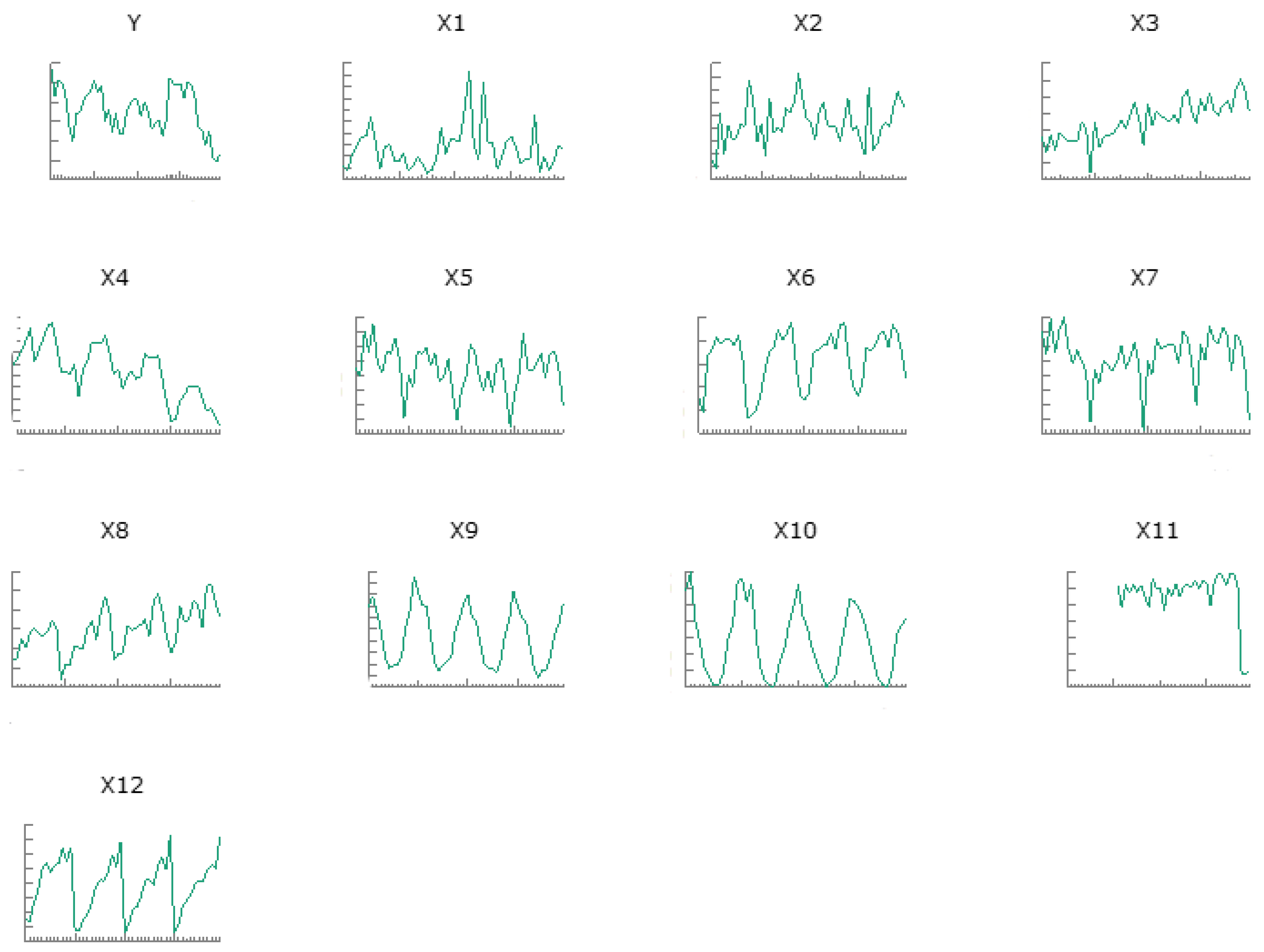
Subsequently, a preliminary analysis of the graphs of the dependence of the explained variable (gas supply to end users) on the explanatory variables, as well as the dependence between the explanatory variables themselves, was carried out. The conclusions of the preliminary analysis showed that the explained variable is dependent.
From all variables, with the exception of the variable ‘price index of industrial production sold.’ Preliminary analysis revealed many unfavourable correlations between the explanatory variables.
Another important aspect was to assess the stationarity of the time series. The variables initially proposed can be used to build the model, but there is a risk of apparent regression. Therefore, the explanatory variable and the explained variables were tested for stationarity. The Dickey-Fuller test for the Y variable showed that it is a series with free expression, linear trend, and quadratic trend. The KPSS test confirmed this fact. The Dickey-Fuller and KPSS tests were used to check trend stability, stationarity, and stochastic nonstationarity for the remaining variables. The results obtained showed that the variables X1, X11, X12, and X13 are stationary. For the period 2016–2018, the series is stationary, it was noted that since the beginning of 2018 there has been a sharp increase for the variable X8, which causes a structural change and these observations were not taken into account.
After examining the series for stationarity, this was removed for the variables for which it was found. A preliminary analysis of the model was then carried out. The estimate of the model was carried out using the classical least-squares method. However, due to the very high p-value for the F-test (0.919), other variables that could be used in the model should be reexamined, as the F-test showed that the variables already proposed would not be able to induce a strong correlation in this system. In addition, an attempt was made to logarithmize the variables, but this did not introduce significant changes in the p-values in the F test. In the search for additional variables, the list of entities classified as final customers was analyzed in terms of their business profile. Furthermore, the zone of customers that have available transmission capacity in the national transmission system was analyzed. Again, the analysis of input data was performed. Based on the analysis of the transmission customers, it can be concluded that entities can be divided into groups: (1) those engaged in the production of basic chemicals, fertilisers and nitrogen compounds, plastics and synthetic rubber in primary forms, (2) those engaged in the sale of heat and natural gas, (3) those engaged in the production of building ceramics and table glass, (4) manufacture of products for the automotive, engineering, and mining industries, (5) manufacture of steel, (6) manufacture of electricity and heat, (6) manufacture of household chemicals, (6) retail, wholesale, (7) other. There is no information available on the volume of gaseous fuel consumption, but from the review of the available literature it can be concluded that the largest amount of gaseous fuel is consumed by industrial customers associated with the production of chemicals, fertilisers, electricity generation, building ceramics and other materials.
A re-analysis of the time series graphs was carried out to check for structural changes in the time series. Descriptive statistics tests were carried out and showed that the variable X1 had a variance of less than 0.1, indicating that this variable alone could not be taken for further analysis.
Next, graphs of the relationship between the explained variable and the nonplanar variables were constructed. After this part, stationarity was reassessed, and non-stationarity was removed from the newly proposed variables.
As a result of the second analysis of the newly proposed variables, the p-value for the test is 0.28. This result could be acceptable due to the values of the Durbin-Watson statistic but the coefficient of determ. The R-square is 0.53, which led the author to decide to combine the variables, from model 1 and model 2, those that have the greatest association strength with the variable under study.
Important information is the fact: the two samples made between January 2016 and March 2018 showed a problem in finding the strength of the relationship between the Y variable.
The third analysis was for the period January 2012–2015. This is the period in which the greatest stabilization was observed. For the next, third attempt at analysis, the following indicators were adopted: production of staple cereals (yields affect phosphate consumption potassium salt, fertilizers), food production (consumers of gaseous fuels), paper production (consumers of gaseous fuels), refined products production (consumers of gaseous fuels), chemicals and chemical products production (consumers of gaseous fuels), manufacture of nonmetallic mineral products (consumers of gaseous fuels), manufacture of basic metals (consumers of gaseous fuels), manufacture of metal products (consumers of gaseous fuels), electricity, gas and steam production and supply, heating days, Continuous power, construction output.
Stationarity estimation and removal of non-stationarity were again performed for the proposed variables in the above setup. Least Squares per-formed estimation suggests removing variables X7, X8, X12-which was done. The following results were obtained:
Having satisfactory variables, a study of the correlation between the variables was made. This test was carried out using a correlation matrix, which shows that variables X9, X10, X11 are potentially strongly related to the explanatory variable Y and describe it well. Furthermore, an additional correlation test between variables was performed using the Hellwig method, which indicated that variables X10 (after stationary trend change) and X11 are the most significant. The integral capacity for this system was 0.42. Due to the correlation between the variables Y and Y9, it was included in the model. In addition, the correlation between the variables was examined using the stepwise regression method (an alternative to Hellwig’s method), which assumed a significance level of 5% for the T-student test. The stepwise regression method showed that the significant explanatory variables for the Y variable were X6, X10, and X11. To sum up the above discussion, the summary variables will be used to build the further model, viz. X6, X9, X10, X11. Based on the tests so far, the batch variables were found to be good.
The model building was then carried out with the relevant variables. A new least squares model was estimated with only four variables already included.
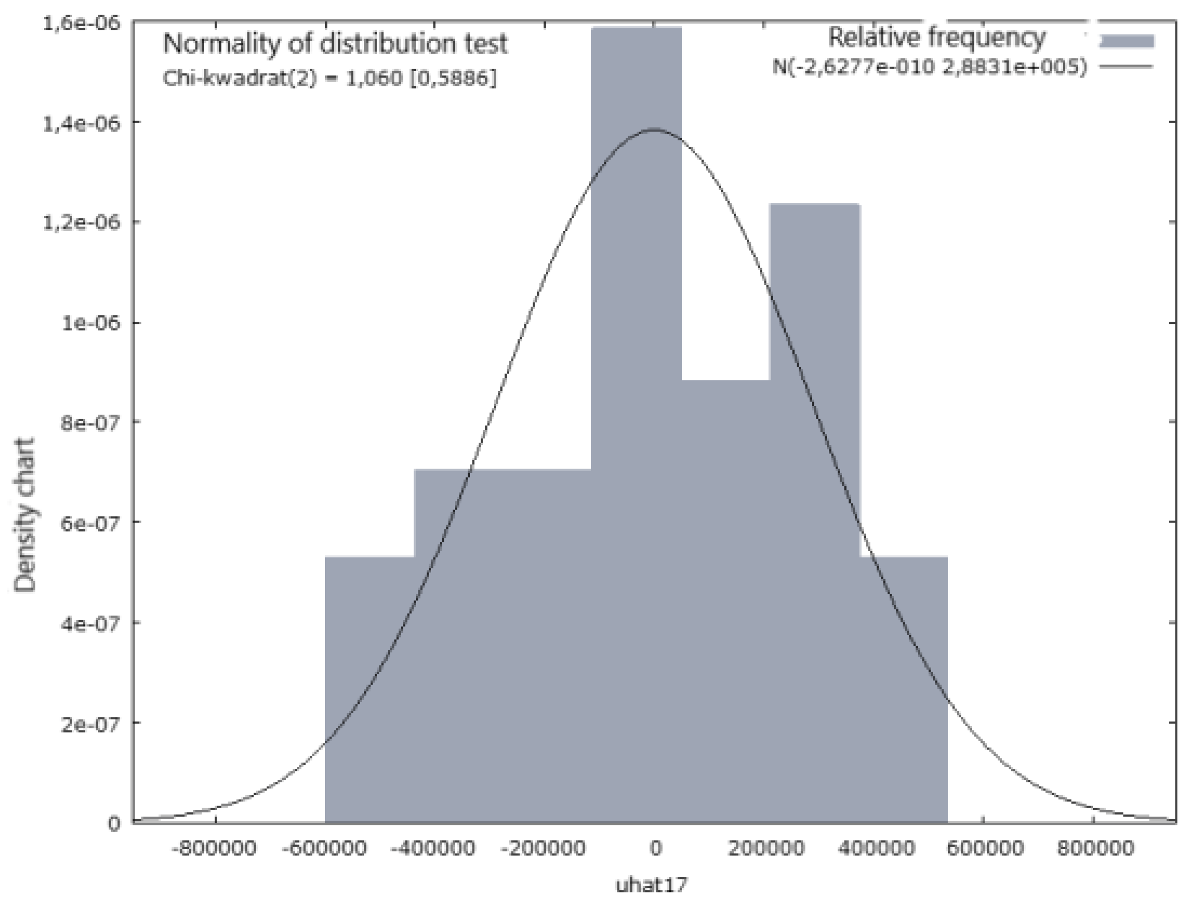
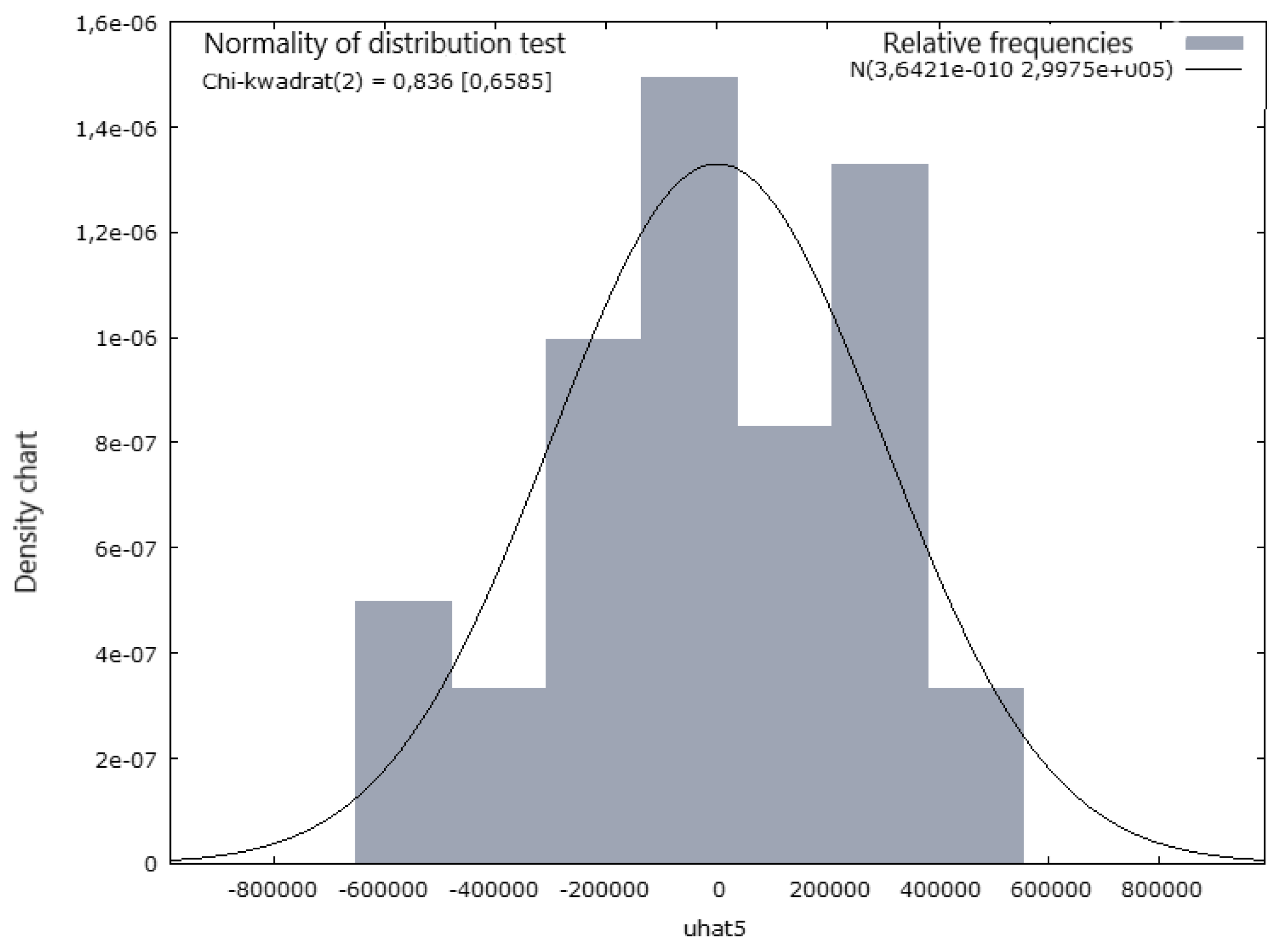
For the new least squares model, the normality distribution of the residuals was checked. The Chi-square test for normality of the distribution and the Doornik-Hansen test showed that the distribution is normal.
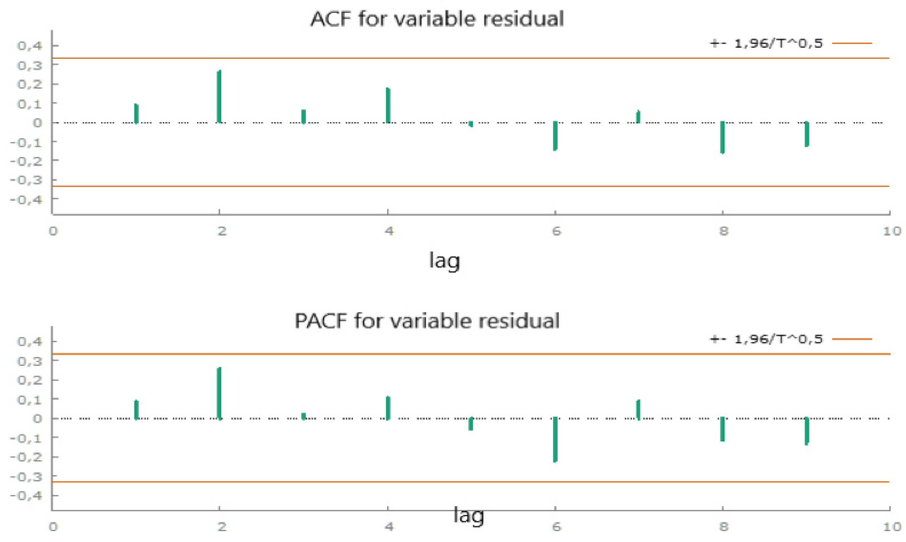
To check for the presence of autocorrelation, the Breusch–Godfrey test based on Lan-grange multipliers was performed, in which the null hypothesis for this test is the absence of autocorrelation. The test carried out showed the absence of autocorrelation (no autocorrelation of the random component), which may indicate a well-done analysis of the input data to the model.
The next point in constructing the model is the test for heteroskedasticity, i.e., the White test and the Breusch-Pagan test were performed to check. The null hypothesis of both tests is the absence of heteroskedasticity. Both tests indicated the absence of the heteroskedasticity problem (p = 0.74).
To further test the fit of the data to the model, the Ramsey RESET test was performed. Null hypothesis: the model is fitted correctly (linearity of the model). The p-value (0.249) indicates that the model is fitted correctly. The collinearity of the variances was further tested with the VIF test. The test was initially conducted for the following variables: X6(after removing trendostationarity), X9, X10 (after removing trendostationarity), X11. The test showed that the highest collinearity occurred for variable X9. The test was repeated for variables X10 (after removing trend stationarity), X11, and X6 (after removing trend stationarity). For these variables, the stepwise regression test and the Hellwig method showed that these were the best variables. Therefore, collinearity was removed. For the new set of variables, the normality test of the residuals, the autocorrelation test, the heteroskedasticity check were performed again. These tests did not show any problems.
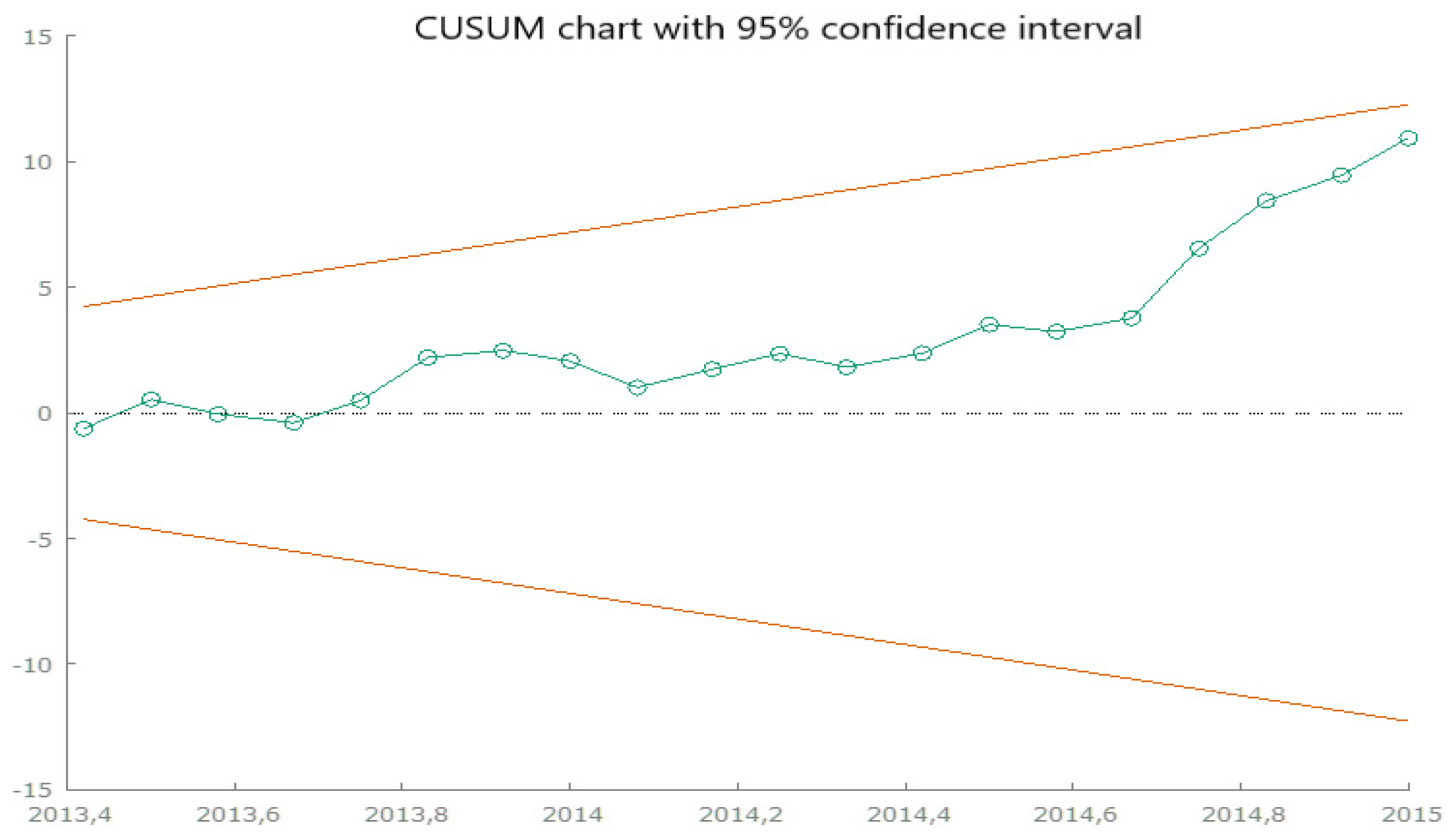
Upon checking the stability of the model parameters, the CUSUM (Cumulated SUM of residuals) test was performed. This test shows whether the index measuring the sensitivity of the model or the sensitivity measure is within the confidence interval, that is, whether the coefficients do not change over time. For three observations, a structural change is visible (not significant-remains unchanged).
In order to improve the stability of the run, a modification related to taking into account structural changes was introduced for variable X 11. Then the whole run formally falls within the confidence interval.
The last step was to conduct a coincidence test, where its absence indicates collinearity of the variables. The coefficients X11_before_shock and X10_filter have the same positive signs, i.e., there is coincidence in the model. The X6_filter has opposite signs. This does not remove it from the model but may introduce some disturbance.

5. Conclusions

Y = 530 , 809 × ( X 6 _ filtr ) + 308 , 393 × ( X 10 _ filtr ) + 11 , 989 × ( X 11 _ before _ shock )
According to the ceteris paribus rule:
The model takes into account:
Y-quantity of gas supplied [MWh/month]
X6-production of mineral fertilizers [ton]
X10-Heating days [index]
X11-contracted firm capacity power [MWh/month].
The volume of gas supplied:
(a)
Increases by 530.809 [MWh] if mineral fertilizer production increases by unit (thousand tonnes) compared to the previous year,
(b)
Is increased by 3083.93 [MWh], if the heating days increase by one unit compared to the previous year,
Heating days (index)—the severity of the cold over a specified period of time, taking into account the outdoor temperature and the average indoor temperature (in other words, the need to heat). HDD calculation is based on a base temperature, defined as the lowest daily average air temperature that does not lead to space heating. The value of the base temperature depends, in principle, on several factors related to the building and its surrounding environment. Using a general climatological approach, the base temperature is set at a constant value of 15 °C in the HDD calculation.
(c)
Will increase by 11,989 MWh if the contracted capacity increases by a unit compared to the previous year.
On the basis of the obtained model of the analysis of interdependence of the natural gas supply phenomenon to customers, it may be concluded that the highest interdependence occurs for the production of mineral fertilizers, the index of the number of days of heating-i.e., the consumption of gaseous fuel by industrial and commercial heat and power plants, and the contracted capacity by the remaining final customers. The other end users are a group with a wide range of production types, so it can be concluded that the tests of the proposed variables did not show a significant impact on the model.
In relation to the actual situation, the model refers to the expected significant increase in the share of gas units, as forecast by Polskie Sieci Elektroenergetyczne. The results of analyses prepared by Polskie Sieci Elektroenergetyczne to determine the future structure of electricity generation for the transmission network development plan update of the for the purpose of updating the transmission network showed a possible significant increase in the number of gas units in the National Power Grid. In addition, activity of entities from the power sector electricity sector may be a result of the emerging power market-the Act of 8 December 2017 on the power market (Dz.U of 2018, item 9) as well as the necessity or willingness to convert in the next few years of highly emitting energy carriers (coal) due to increasing electricity demand.
Charges for CO2, NOX, etc. emissions. The analysis of the interdependence of the observed phenomenon and the construction of the model provides information on the important factors influencing the consumption of natural gas by the Polish industry and their impact on this effect. It can provide knowledge, decision makers, politicians, distribution and transmission operators in making decisions related to the construction of infrastructure and other business operations. Econometric models can be successfully implied in energy companies conducting business related to energy trading. Such models will allow them to understand market phenomena and investigate the reasons behind the industry’s interest in energy.
The application of this model can be used by energy companies involved in trading, supplying gaseous fuels to end consumers. Energy operators will pay attention to the most important external indicators influencing natural gas off-take. This knowledge determines the proposed parameters to which particular attention should be paid, in planning the supply of natural gas to consumers. The article outlines the essence of macroeconomic modeling as one that can complement mechanical forecasting based on historical data. The model clearly indicated that the largest consumption of natural gas in Poland is related to the commercial power industry, heat engineering and switching economies from coal to, i.a., natural gas.
The selection of potential macroeconomic indicators should be critically assessed. The pre-selection of potential explanatory variables is time-consuming and the analyst must have a working knowledge of the market under study. Macroeconomic modeling is also unable to build a model capable of signaling the accumulation of negative economic phenomena.
Future directions of research should include identification of the most significant factors influencing the consumption of natural gas by the Polish economy as a result of the ongoing energy transition in order to achieve carbon neutrality. This research could also be based on the time period during which the coronavirus pandemic occurred and affected the reduction of energy consumption by end users. Future research could also indicate how the pandemic directly affected the analyzed macroeconomic indicators, which subsequently affected energy consumption. Furthermore, the research procedure presented can also be applied to other energy sectors. A challenge for today may be to present this method in the area of renewable energy sources. An interesting challenge is the development of an econometric model covering all available energy sources and their combination with the development of a forecast. It is also worth undertaking other studies to analyze macroeconomic indicators for different countries of the European Union and to develop models with comparisons, while checking which indicators affect which countries. The results of this research could be the subject of a fair energy transition.

Author Contributions

Conceptualization, T.C. and M.Ł.; methodology, T.C.; software, T.C.; validation, T.C. and M.Ł.; formal analysis, T.C.; investigation, M.Ł.; resources, T.C.; data curation, T.C.; writing—original draft preparation, T.C.; writing—review and editing, T.C.; visualization, T.C.; supervision, M.Ł.; project administration, T.C.; funding acquisition, M.Ł. All authors have read and agreed to the published version of the manuscript.

Funding

This research received no external funding.

Institutional Review Board Statement

Not applicable.

Informed Consent Statement

Not applicable.

Data Availability Statement

Not applicable.

Conflicts of Interest

The authors declare no conflict of interest.

References

  1. Deligeorgiou, G.; Gounaris, K. Natural Gas as a Source of Energy. In Proceedings of the Conference on Advances in Management, Economics and Social Science–MES 2014, Rome, Italy, 7–8 June 2014. [Google Scholar] [CrossRef]
  2. Latif, S.A.; Chiong, M.; Rajoo, S.; Takada, A.; Chun, Y.-Y.; Tahara, K.; Ikegami, Y. The Trend and Status of Energy Resources and Greenhouse Gas Emissions in the Malaysia Power Generation Mix. Energies 2021, 14, 2200. [Google Scholar] [CrossRef]
  3. Bisaga, I.; To, L. Funding and Delivery Models for Modern Energy Cooking Services in Displacement Settings: A Review. Energies 2021, 14, 4176. [Google Scholar] [CrossRef]
  4. IEA. Special Report on World Energy Outlook. The Role of Gas in Today’s Energy Transitions; IEA: Paris, France, 2019; Available online: https://www.iea.org/reports/the-role-of-gas-in-todays-energy-transitions/ (accessed on 29 July 2021).
  5. PEP 2040. Available online: https://www.gov.pl/web/klimat/polityka-energetyczna-polski-do-2040-r-przyjeta-przez-rade-ministrow/ (accessed on 29 July 2021).
  6. Gawlik, L.; Mokrzycki, E. Paliwa kopalne w krajowej energetyce—Problemy i wyzwania. Polityka Energetyczna—Energy Policy J. 2017, 20, 5–25. [Google Scholar]
  7. NATO. Energy Security: Operational Highlights; NATO: Brussels, Belgium; Volume 15, Available online: https://www.enseccoe.org/data/public/uploads/2021/08/nato-ensec-coe-energy-highlights-no.15.pdf/ (accessed on 29 July 2021).
  8. Hong, L.; Zhang, H.; Xie, J.; Wang, D. Analysis of factors influencing the Henry Hub natural gas price based on factor analysis. Pet. Sci. 2017, 14, 822–830. [Google Scholar]
  9. Hasterok, D.; Castro, R.; Landrat, M.; Pikoń, K.; Doepfert, M. Polish Energy Transition 2040: Energy Mix Optimization Using Grey Wolf Optimizer. Energies 2021, 14, 501. [Google Scholar] [CrossRef]
  10. Smith, L.V.; Tarui, N.; Yamagata, T. Assessing the impact of COVID-19 on global fossil fuel consumption and CO2 emissions. Energy Econ. 2021, 97, 105170. [Google Scholar] [CrossRef] [PubMed]
  11. Mugableh, M.I. The Relationships between Energy Consumption and Economic Growth: A Review of the Literature. J. Econ. Manag. Res. 2020, 8, 1–2. [Google Scholar] [CrossRef]
  12. Radmehr, R.; Henneberry, S.R.; Shayanmehr, S. Renewable Energy Consumption, CO2 Emissions, and Economic Growth Nexus: A Simultaneity Spatial Modeling Analysis of EU Countries. Struct. Chang. Econ. Dyn. 2021, 57, 13–27. [Google Scholar] [CrossRef]
  13. Abbasi, K.R.; Hussain, K.; Abbas, J.; Adedoyin, F.F.; Shaikh, P.A.; Yousaf, H.; Muhammad, F. Analyzing the role of industrial sector’s electricity consumption, prices, and GDP: A modified empirical evidence from Pakistan. AIMS Energy 2021, 9, 29–49. [Google Scholar] [CrossRef]
  14. Gershon, O.; Emekalam, P. Determinants of Renewable Energy Consumption in Nigeria: A Toda Yamamoto Approach. IOP Conf. Ser. Earth Environ. Sci. 2021, 665, 012005. [Google Scholar] [CrossRef]
  15. Li, C. Macroeconomic Short-Term High-Precision Combined Forecasting Algorithm Based on Grey Model. Secur. Commun. Netw. 2021, 2021, 1–9. [Google Scholar] [CrossRef]
  16. He, Y.; Collins, A.R. Optimal dynamic electricity consumption function estimation: An institutional experimental evidence from Guangzhou, China (1949–2016). Econ. Res.-Ekon. Istraživanja 2021, 34, 1–25. [Google Scholar] [CrossRef]
  17. Ghosh, P.K.; Manna, A.K.; Dey, J.K.; Kar, S. Supply chain coordination model for green product with different payment strategies: A game theoretic approach. J. Clean. Prod. 2021, 290, 125734. [Google Scholar] [CrossRef]
  18. Catalán, H. Impacto de las energías renovables en las emisiones de gases efecto invernadero en México. Probl. Desarro. 2020, 52, 59–83. [Google Scholar] [CrossRef]
  19. Bulkani; Sonedi; Chandra; Anugrah; Putra. The Natural Gas Consumption and Economic Development Nexus: Fresh Evidence from Indonesia. Int. J. Energy Econ. Policy 2021, 11, 607–614. [Google Scholar] [CrossRef]
  20. Etokakpan, M.U.; Solarin, S.A.; Yorucu, V.; Bekun, F.V.; Sarkodie, S.A. Modeling natural gas consumption, capital formation, globalization, CO2 emissions and economic growth nexus in Malaysia: Fresh evidence from combined cointegration and causality analysis. Energy Strat. Rev. 2020, 31, 100526. [Google Scholar] [CrossRef]
  21. Harkat; Tahar. The Impact of Natural Gas Consumption on Industry Value Added in the Mediterranean Region; Munich Personal RePEc Archive: Munich, Germany, 2019; Available online: https://mpra.ub.uni-muenchen.de/92492/1/MPRA_paper_92492.pdf/ (accessed on 27 July 2021).
  22. Makala, D.; Zongmin, L. Natural Gas Consumption and Economic Growth in Tanzania. Eur. J. Sustain. Dev. Res. 2019, 4, em0113. [Google Scholar] [CrossRef] [Green Version]
  23. Rusev, V.N.; Abramkin, G.V.; Muravyova, E.K. Multiple regression model for gas consumption in Germany. IOP Conf. Ser. Earth Environ. Sci. 2021, 808, 012033. [Google Scholar] [CrossRef]
  24. Martinez-Castillo, C.; Astray, G.; Mejuto, J. Modelling and Prediction of Monthly Global Irradiation Using Different Prediction Models. Energies 2021, 14, 2332. [Google Scholar] [CrossRef]
  25. Han, H.; Picoli, G.J., Jr.; Gue, H.; Yu, Q.; Powles, S.B. Mechanistic basis for synergism of 2,4-D amine andmetribuzin in Avena sterilis. J. Pestic. Sci. 2020, 45, 216–222. [Google Scholar] [CrossRef]
  26. Sobczyk, M. Ekonometria; Wydawnictwo, C.H., Ed.; Beck: Warszawa, Poland, 2013; p. 9. [Google Scholar]
  27. Jialinang, W.; Nu, L. Influencing factors and future trends of natural gas demand in the eastern, central and western areas of China based on the grey model. Nat. Gas Ind. B 2020, 7, 473–483. [Google Scholar]
  28. Wildan, M.A.; Imron, M.A.; Siswati, E.; Rosyafah, S. Macroeconomic factors affecting natural gas export management. Int. J. Energy Econ. Policy 2020, 11, 639–644. [Google Scholar] [CrossRef]
  29. Gao, F.; Shao, X. Forecasting annual natural gas consumption via the application of a novel hybrid model. Environ. Sci. Pollut. Res. 2021, 28, 21411–21424. [Google Scholar] [CrossRef]
  30. Botzen, W.; Nees, T.; Estrada, F. Temperature Effects on Electricity and Gas Consumption: Empirical Evidence from Mexico and Projections under Future Climate Conditions. Sustainability 2020, 13, 305. [Google Scholar] [CrossRef]
  31. Factors Affecting Natural Gas Prices. Available online: https://www.eia.gov/energyexplained/natural-gas/factors-affecting-natural-gas-prices.php (accessed on 29 July 2021).
  32. Rubaszek, M.; Bech-Wysocka, K.; Dybka, P. Skrypt do Przedmiotu Ekonometria I; Szkoła Główna Handlowa w Warszawie: Warszawa, Poland, 2020. [Google Scholar]
  33. Cottrell, A.; Lucchetti, R. Gretl User ManualGretl User Manual. 2007. Available online: http://gretl.sourceforge.net/ (accessed on 25 July 2021).
  34. Bex, T. How to Remove Non-Stationarity in Time Series Forecasting. Available online: https://towardsdatascience.com/how-to-remove-non-stationarity-in-time-series-forecasting-563c05c4bfc7 (accessed on 29 July 2021).
  35. Champion, R.; Lenard, C.T.; Mills, T.M. Demonstrating the Durbin-Watson Statistic. J. R. Stat. Soc. Ser. D Stat. 1998, 47, 643–644. [Google Scholar] [CrossRef]
  36. Riffenburgh, R. Sequential Analysis and Time Series. Statistics in Medicine, 3rd ed.; Academic Press: Cambridge, MA, USA, 2012. [Google Scholar]
  37. Bozdogan, H. Model selection and Akaike’s Information Criterion (AIC): The general theory and its analytical extensions. Psychometrika 1987, 52, 345–370. [Google Scholar] [CrossRef]
  38. Cheng, C.-L.; Shalabh; Garg, G. Coefficient of determination for multiple measurement error models. J. Multivar. Anal. 2014, 126, 137–152. [Google Scholar] [CrossRef] [Green Version]
  39. Pham-Gia, T.; Choulakian, V. Distribution of the Sample Correlation Matrix and Applications. Open J. Stat. 2014, 4, 330–344. [Google Scholar] [CrossRef] [Green Version]
  40. Using Gretl for Principles of Econometrics. Available online: http://www.kufel.torun.pl/prog/ebook_gretl.pdf (accessed on 29 July 2021).
  41. Smith, G. Step away from stepwise. J. Big Data 2018, 5, 32. [Google Scholar] [CrossRef]
  42. Farbmacher, H.; Kögel, H. Testing under a special form of heteroscedasticity. Appl. Econ. Lett. 2016, 24, 264–268. [Google Scholar] [CrossRef]
  43. Breusch, T.; Pagan, R. A simple test for heteroscedasticity and random coefficient variaton. Econometrica 1979, 47, 5. [Google Scholar] [CrossRef]
  44. Akinwande, M.O.; Dikko, H.G.; Samson, A. Variance Inflation Factor: As a Condition for the Inclusion of Suppressor Variable(s) in Regression Analysis. Open J. Stat. 2015, 5, 754–767. [Google Scholar] [CrossRef] [Green Version]
  45. Belsley, D. A Guide to using the collinearity diagnostics. Comput. Sci. Econ. Manag. 1991, 4, 33–50. [Google Scholar]
Figure 1. Supply of natural gas to the Polish transmission system from national production (2016–2021). These data can be found here: https://www.entsog.eu/ (accessed on 1 October 2021).
Energies 14 07649 g001
Figure 2. Supply of natural gas to Polish customers (2011–2015). This data can be found here: https://www.entsog.eu/ (accessed on 1 October 2021).
Energies 14 07649 g002
Figure 3. Procedure for constructing an econometric model.
Energies 14 07649 g003
Figure 4. Supply of natural gas to Polish customers (2011–2015). This data can be found here: https://www.entsog.eu/ (accessed on 1 October 2021).
Energies 14 07649 g004
Figure 5. Graph of the variables time series of the analysed variables in the period 2011–2015. This data can be found here: https://ec.europa.eu (accessed on 1 October 2021).
Energies 14 07649 g005
Figure 6. Normality of distribution test.
Energies 14 07649 g006
Figure 7. ACF and PACF for variable residual.
Energies 14 07649 g007
Figure 8. ACF and PACF for variable residual (2).
Energies 14 07649 g008
Figure 9. CUSUM Test Harvey-Collier test statistic = 2.44718 with p-value = 0.02429.
Energies 14 07649 g009
Table 1. Volume of recoverable natural gas reserves from gas, oil, and condensate fields in mln m3 (own elaboration based on data from Polish Geological Institute).
YearQuantity of ReservoirsMines ResourcesOff-Balance ReservoirsIndustrial Resources
2020306141,643.382277.1373,514.38
2019305141,971.362277.6774,953.67
2018298139,929.312230.5966,640.98
2017295116,956.982230.2650,607.8
2016293119,721.342219.8552,295.1
Table 2. The preliminary macroeconomic indicators proposed.
The Macroeconomic Indicators Proposed
YNatural gas consumption by end consumers
X1Primary cereal production (yields affect potassium phosphate production potassium
X2Production of foods (consumers of gaseous fuel)
X3Paper production (consumers of gaseous fuel)
X4production of refined products (consumers of gaseous fuel)
X5Manufacture of chemicals and chemical products (consumers of gasoline)
X6Manufacture of nonmetallic mineral products (consumers of gasoline)
X6Metal production (consumers of gaseous fuel)
X7Manufacture of metal products (consumers of gaseous fuels)
X8Electricity, gas, steam, and air conditioning supply
X9Heating days
X10Contracted firm capacity in the National Natural Gas Transmission System
X11Building production
Table 3. Method of least squares (Model 1). Observations used 02.2013–12.2015 (N = 35).
RatioStandard Errort-Studentp-ValueInfluence (0–3)
const−3.14543 × 1061.36906 × 106−2.2980.0296**
X2−193.03497.8029−1.9740.0587*
X5889.485316.0732.8140.0090***
X71407.52467.0173.0140.0056***
X8−823.527313.236−2.6290.0140**
X103218.41363.6318.851<0.0001***
X1111.66402.093055.573<0.0001***
X12323.16891.07263.5480.0014***
Table 4. Determined parameters (Model 1).
Determined Parameters
Arithmetic mean of the dependent variable4,194,017Standard deviation of the subsidiary599,008.3
Sum of squares of the residuals1.86 × 1012Standard error of residuals262,753.9
Coefficient of determination R-square0.847202Corrected R-square0.807588
F(7, 27)21.38628The p-value for the F-test1.80 × 10−9
Logarithm of reliability−481.8855Crit. inform. Akaike’s979.7709
The Bayes–Schwarz criterion992.2137Crit. Hannan–Quinn984.0662
Autocorrelation of residuals-rho1−0.037921Stat. Durbin–Watson2.035796
Table 5. Determination of Stationarity and Removal of Stationarity from Time Series Data.
Verification of stationarity
p valueX1X2X3X4X5X6X7X8X9X10X11X12
Extended Dickey-Fuller test0.8670.97410.9220.5260.0060.6850.9830.0010.9990.993
KPSS test for the variable>0.10>0.10 >0.10>0.10>0.10>0.100.012>0.100.83>0.10>0.10
Verification of the removal of non-stationarity
X1X2X3X4X5X6X7X8X9X10X11X12
Extended Dickey-Fuller test0.0360.0070.0010.0470.001 0.0030.001 0.004
KPSS test for the variable>0.10>0.10>0.10>0.10>0.10 >0.10>0.10>0.10>0.10
Table 6. Method of least squares), for the factors listed below.
RatioStandard Error.t-Studentp-ValueInfluence (0–3)
const−2.70592 × 1063.87983 × 106−0.69740.4925
X3_filtr−1824.80908.311−2.0090.0564*
X4_filtr196.094105.4121.8600.0757*
X6_filtr1289.20578.5632.2280.0359**
X8_filtr−430.428337.782−1.2740.2153
X10_filtr2510.351339.851.8740.0737*
X2−228.683121.376−1.8840.0723*
X5385.415415.7210.92710.3635
X7488.963458.4371.0670.2972
X9485.849226.9072.1410.0431**
X1111.13532.171785.127<0.0001***
X120.28360876.08160.0037280.9971
Table 7. Determined parameters.
Arithmetic mean of the dependent variable4,194,017Standard deviation of the subsidiary599,008.3
Sum of squares of the residuals1.61 × 1012Standard error of residuals264,928.0
Coefficient of determination R-square0.867676Corrected R-square0.804390
F(7, 27)13.71051The p-value for the F-test1.29 × 107
Logarithm of reliability−479.3679Crit. inform. Akaike’s982.7358
The Bayes–Schwarz criterion1001.400Crit. Hannan–Quinn989.1786
Autocorrelation of residuals-rho10.054622Stat. Durbin–Watson1.884526
Table 8. Method of least squares (Model 3), following differentiation.
RatioStandard Error.t-Studentp-ValueInfluence (0–3)
const−9.80418 × 1063.87983 × 106−2.730.0118**
X2−259.607112.11−2.310.0298**
X3_filtr−1540.75838.93−1.830.0792*
X4_filtr165.8197.361.710.1020
X5629.01383.961.630.1150
X6_filtr889.15534.371.660.1097
X71185.38423.422.80.0102**
X8_filtr−734.75311.98−2.350.0274**
X9362.48209.571.70.0971*
X102833.151237.512.280.0316**
X119.722.014.84<0***
X12162.8170.272.310.0298**
Table 9. Determined parameters (Model 3), following differentiation.
Arithmetic mean of the dependent variable188.14Standard deviation of the subsidiary576,185.7
Sum of squares of the residuals1.38 × 1012Standard error of residuals244,692.4
Coefficient of determination R-square0.877999Corrected R-square0.819650
F(7, 27)15.04749The p-value for the F-test5.33 × 10−8
Logarithm of reliability−476.5869Crit. inform. Akaike’s977.1738
The Bayes–Schwarz criterion995.83Crit. Hannan–Quinn983.6167
Autocorrelation of residuals-rho1−0.067004Stat. Durbin–Watson2.100575
Table 10. Method of matrix analysis of correlation coefficients.
Y_filtrX2X3_filtrX4_filtrX5
1.0000−0.1876−0.0161−0.1095−0.0861Y_filtr
1.00000.58940.35510.3468X2
1.00000.35720.5419X3_filtr
1.00000.1363X4_filtr
1.0000X5
X6_filtrX7X8_filtrX9X10_filtr
−0.33180.1026−0.22000.44580.4954Y_filtr
0.43670.15480.66630.0958−0.0159X2
0.50770.66850.6754−0.0431−0.0847X3_filtr
0.71410.35210.5914−0.5176−0.5994X4_filtr
0.55310.72080.5235−0.3794−0.3274X5
1.00000.61840.8392−0.7728−0.8225X6_filtr
1.00000.5725−0.4988−0.3957X7
1.0000−0.4002−0.4494X8_filtr
1.00000.9542X9
1.0000X10_filtr
X11X12
0.4851−0.2345Y_filtr
−0.35180.4484X2
−0.1275−0.0080X3_filtr
0.27100.3822X4_filtr
−0.0116−0.3133X5
0.11990.3826X6_filtr
0.2430−0.2931X7
−0.13440.4815X8_filtr
−0.2822−0.1002X9
−0.2877−0.2301X10_filtr
1.0000−0.2482X11
1.0000X12
Table 11. Stepwise Regression Method.
Non-Significant Variable Eliminatedp-Value
X50.115
X4_filtr0.317
X20.101
X90.168
X120.085
X8_filtr0.212
X70.055
X3_filtr0.153
Table 12. Method of least squares (Model 4), following differentiation.
RatioStandard Errort-Studentp-ValueInfluence (0–3)
const−3.7127 × 106477104−7.7828.83 × 10−9***
X6_filtr544.198173.4543.1370.00037***
X10_filtr3312.34490.0656.7591.45 × 10−7***
X1113.7541.7527.8477.42 × 10−9***
Table 13. Determined parameters (Model 4), following differentiation.
Arithmetic mean of the dependent variable188.14Standard deviation of the subsidiary576,185.7
Sum of squares of the residuals2.79 × 1012Standard error of residuals299,753.9
Coefficient of determination R-square0.7532Corrected R-square0.7293
F(7, 27)31.54The p-value for the F-test1.52 × 10−9
Logarithm of reliability−488.9141Crit. inform. Akaike’s985.82
The Bayes–Schwarz criterion992.0497Crit. Hannan–Quinn987.975
Autocorrelation of residuals-rho10.232Stat. Durbin–Watson1.5258
Table 14. Method of least squares (Model 5), following differentiation.
RatioStandard Errort-Studentp-ValueInfluence (0–3)
const−2.46833 × 1061.30751 × 106−1.8880.0688*
X6_filtr555.933173.7093.2000.0032***
X9−152.861149.549−1.0220.3149
X10_filtr4195.20992.9034.2250.0002***
X1113.73281.751677.840<0.0001***
Table 15. Determined parameters (Model 5), following differentiation.
Arithmetic mean of the dependent variable188.1458Standard deviation of the subsidiary576,185.7
Sum of squares of the residuals2.69 × 1012Standard error of residuals299,537.7
Coefficient of determination R-square0.761537Corrected R-square0.729742
F(7, 27)23.95148The p-value for the F-test5.70 × 10−9
Logarithm of reliability−488.3151Crit. inform. Akaike’s986.6301
The Bayes–Schwarz criterion994.4068Crit. Hannan–Quinn989.3146
Autocorrelation of residuals-rho10.151076Stat. Durbin–Watson1.678929
Table 16. Indicators characterizing the density graph.
RangesAverageNumberCumulative
Frequency
Influence (0–10)
< 4.370 × 10⁵−5.181 × 10538.57%8.57%***
−4.370 × 10⁵−2.749 × 10⁵−3.560 × 105411.43%20.00%****
−2.749 × 10⁵−1.128 × 10⁵−1.938 × 105411.43%31.43%****
−1.128 × 1054.932 × 104−3.173 × 104925.71%57.14%*********
4.932 × 1042.114 × 1051.304 × 105514.29%71.43%*****
2.114 × 1053.735 × 1052.925 × 105720.00%91.43%*******
>=3.735 × 1054.546 × 10538.57%100.00%***
Table 17. Heteroskedasticity test (Breusch–Pagan test).
RatioStandard Errort-Studentp-Value
const−0.7487455.32835−0.14050.8892
X6_filtr0.0009027390.0007078961.2750.2120
X9−8.08896 × 10−50.000609442−0.13270.8953
X10_filtr0.002991760.004046270.73940.4654
X118.92825 × 10−67.13837 × 10−61.2510.2207
Table 18. Technical diagnosis of the model (Test Ramsey Reset).
RatioStandard Errort-Studentp-ValueInfluence
(0–3)
const−3.50085 × 1061.48998 × 106−2.3500.0261**
X6_filtr710.953217.7373.2650.0029***
X9−235.476156.804−1.5020.1444
X10_filtr5279.771349.623.9120.0005***
X1119.68574.611774.2690.0002***
yhat^23.36764 × 10−72.58559 × 10−71.3020.2034
yhat^3−5.32538 × 10−134.76748 × 10⁻¹³−1.1170.2735
Table 19. Stability test for coefficients.
CoefficientValue
X6_filtr3.254
X911.222
X10_filtr14.310
X111.143
Table 20. Variance proportions (1).
LambdaCondConstX6_filtrX9X10_filtrX11
2.9811.0000.0000.0000.0000.0000.001
1.8301.2760.0000.0830.0000.0190.000
0.1804.0660.0000.8580.0000.1860.000
0.00819.6330.0250.0580.0440.1260.949
0.00160.2810.9750.0010.9550.6690.049
Table 21. Number of condition indicators for cond >= 10:2. Sum of the proportion of variance >= 0.5 for cond >= 10.
ConstX9X10_filtrX11
1.0001.0000.7950.998
Table 22. Repeated test for variables X10_filter, X11, X6_filter.
X10_filtr3.481
X111.143
X6_filtr3.239
Table 23. Variance proportions (2).
LambdaCondConstX10_filtrX11X6_filtr
1.9981.0000.0030.0020.0030.001
1.8181.0480.0000.0770.0000.084
0.1783.3550.0000.8050.0000.867
0.00618.8530.9970.1160.9970.048
Table 24. Number of condition indicators for cond >= 10:2. Sum of the proportion of variance >= 0.5 for cond >= 10 (2).
ConstX11
0.9970.997
Table 25. Indicators characterizing the density graph (2).
RangesAverageNumberCumulative
Frequency
Influence
(0–10)
<−4.800 × 10⁵−5.659 × 10538.57%8.57%***
−4.800 × 10⁵−3.080 × 10⁵−3.940 × 10525.71%14.29%**
−3.080 × 10⁵−1.360 × 10⁵−2.220 × 105617.14%31.43%******
−1.360 × 1053.597 × 104−5.002 × 104925.71%57.14%*********
3.597 × 1042.080 × 1051.220 × 105514.29%71.43%*****
2.080 × 1053.799 × 1052.939 × 105822.86%94.29%********
>= 3.799 × 1054.659 × 10525.71%100.00%**
Table 26. Test for Autocorrelation.
CoefficientStandard Errort-Studentp-Value
const177,7542.15508 × 1060.082480.9352
X11−0.8718767.71008−0.11310.9112
X6_filtr−69.2738224.845−0.30810.7615
X10_filtr−320.516619.034−0.51780.6109
X11_after_shock1.935494.776900.40520.6901
uhat_10.01814160.2665580.068060.9465
uhat_20.2320330.2403890.96520.3472
uhat_30.06300020.2540430.24800.8069
uhat_40.2987620.2505911.1920.2487
uhat_50.1143090.2806570.40730.6886
uhat_6−0.1207950.323099−0.37390.7129
uhat_70.2174870.2902350.74930.4633
uhat_8−0.06253700.273920−0.22830.8220
uhat_9−0.2461560.260332−0.94550.3569
uhat_10−0.2441250.270089−0.90390.3780
uhat_11−0.2294350.291265−0.78770.4411
uhat_12−0.3583310.300190−1.1940.2481
Table 27. Test for heteroskedasticity (2).
CoefficientStandard Errort-Studentp-Value
const5.32132 × 10111.43860 × 10120.36990.7146
X11−4.16140 × 1061.12841 × 107−0.36880.7154
X6_filtr−1.38702 × 1086.13871 × 108−0.22590.8231
X10_filtr−1.17824 × 1093.63169 × 109−0.32440.7483
sq_X119.6196922.12810.43470.6675
X2_X3709.9192214.870.32050.7512
X2_X44837.7712,932.60.37410.7115
sq_X6_filtr−167,636165,722−1.0120.3214
X3_X4−990,056907,689−1.0910.2858
sq_X10_filtr−1.85355 × 1061.57325 × 106−1.1780.2498
Table 28. Final model-parameters.
CoefficientStandard Errort-Studentp-ValueInfluence (0–3)
const−3.26338 × 1061.82076 × 106−1.7920.0882*
X6_filtr530.809221.6272.3950.0265**
X10_filtr3083.93627.1744.917<0.0001***
X11_per_shock11.98926.561591.8270.0826*
Table 29. Determined parameters (Final Model).
Arithmetic mean of the dependent variable33,489.86Standard deviation of the subsidiary509,542.0
Sum of squares of the residuals2.05 × 1012Standard error of residuals319,805.6
Coefficient of determination R-square0.657458Corrected R-square0.606076
F(7, 27)12.79565The p-value for the F-test0.000068
Logarithm of reliability−336.0779Crit. inform. Akaike’s680.1558
The Bayes–Schwarz criterion684.8680Crit. Hannan–Quinn681.4060
Autocorrelation of residuals-rho10.115482Stat. Durbin–Watson1.712620
Table 30. Coincidence test (Final Model).
X6_filtr530.809
X10_filtr3083.93
X11_per_shock11.9892
Table 31. Coincidence test (2) (final model).
Y_filtrX6_filtrX11_per_shockX10_filtr
1.00000.39940.11140.6906
Publisher’s Note: MDPI stays neutral with regard to jurisdictional claims in published maps and institutional affiliations.

