Thermo-Hydraulic Characteristics of Micro-Scale Surface Roughness Topology of Additively Manufactured Surface Model: Modal Decomposition Perspective

Abstract

As a consequence of rapid development of additive manufacturing (3D printing) methods, the academic/industrial demand has been continuously increasing. One field of application is the manufacturing of heat exchanging devices using this promising method. In this regard, understanding the underlying mechanisms from a thermo-hydraulic viewpoint becomes important. Therefore, in this study, scale-resolving large eddy simulation (LES) is applied to reveal the flow details in combination with a model of roughness topology occurring in additive manufacturing. To process the transient LES results, proper orthogonal decomposition (POD) is used to extract the coherent flow structures, and the extended POD is used to rank the flow modes based on thermal importance. The main aim of the present work is to go beyond the conventionally applied methodologies used for the evaluation of surface roughness, i.e., averaged numerical study or experimental overall performance evaluation of the flow/thermal response of additively manufactured surfaces in heat exchangers. This is necessary to reveal the underlying flow mechanisms hidden in the conventional studies. In this study, the behavior of the flow over the micro-scale surface roughness model and its effects on heat transfer are studied by assuming cone-shaped roughness elements with regular placement as the dominant surface roughness structures. The major discussions reveal the footprint of flow mechanisms on the heat transfer coefficient spatial modes on the rough surface. Moreover, comparative study on the flow/thermal behavior at different levels of roughness heights shows the key role of the height-to-base-diameter ratio of the roughness elements in thermal performance.

1. Introduction

The trending additive manufacturing 3D printing method has been recognized as a solution to manufacture light-weight/compact heat exchanging devices with minimized material waste and facilitation of freedom in designing complex elements. Generally, the technology applies the additive shaping principle. As a result, the three-dimensional body is made by successive addition of material [1]. The term ‘additive’ opposes the conventional ‘subtractive’ manufacturing methods, where selective removal of material is used to build the specific shape of bodies. Examples are milling, turning, and drilling [1]. In fact, in additive manufacturing, a part is built by layer-by-layer material addition, minimizing the overall waste of raw material [2]. Selective laser sintering, selective laser melting (very similar to selective laser sintering and differing primarily in the materials they use), electron beam melting, and direct metal laser sintering are the additive manufacturing methods dealing with metals [3,4].

One feature of 3D-printed heat exchanging devices that is important to thermal performance is the minimization of contact thermal resistance caused by conventional attachment of elements on surfaces [4]. Aside from the plus points, the challenges of the additive manufacturing must be considered; overhang printing, removal of supporting structures, compatible raw materials, and minimization of the overall costs can be named as a few [2]. In addition to the mentioned positive and challenging features, the process-induced surface roughness of additive manufacturing-enabled materials has become a topic from the perspective of fluid mixing and heat transfer consequences [5].

The growing trend of 3D printing technology in manufacturing heat exchanging and thermal management devices on the one hand, and the naturally rough surface of the 3D-printed parts on the other hand make the study of the surface roughness effect on the thermo-hydraulic performance of additively manufacturing heat exchangers a critical topic. Stimpson et al. [5] evaluated the surface roughness produced by the direct metal laser sintering process and measured its influence on flow losses and convective heat transfer through rectangular minichannels. Their work contains experimental data to study the overall performance of the rough surface in terms of the pressure loss and heat transfer coefficient. However, the detailed study of flow/thermal behavior is missing. The numerical study of rough surface effects on thermo-hydraulic performance has been conducted through both averaged models and detailed flow study methods, such as direct numerical simulation (DNS) and large eddy simulation (LES). Isaev et al. [6] provided a numerical study based on Reynolds averaged Navier Stokes (RANS) turbulence modelling on vortex heat transfer enhancement in the presence of oval-trench surface dimples. The focus of this study was on the mechanism of secondary flow restructuring and heat transfer enhancement due to the formation of vortex structures in the dimples and spiral vortices in behind. Despite the undeniable strength of RANS/URANS in providing desirably fast study of engineering cases in the presence of a turbulent flow regime, there are research items reporting unrealistic results obtained by such models in comparison to the scale-resolving LES model and DNS. Turnow et al. [7] provided a study on the flow structures and heat transfer in a staggered array of dimples on a surface in the presence of turbulent flow. They reported the flow structures determined by LES inside the dimple as chaotic, containing a wide range of scales where coherent structures are hard to detect. The applied POD showed tornado-like flow structures, and the different geometrical configurations of the dimples on the surface were shown to have considerable capacity to control the dimple-induced flow mixing.

Among the methods of analyzing the numerical/experimental data of turbulent flow thermal fields, POD has attracted considerable attention. Lumley [8] proposed this method in the field of fluid dynamics. The primary idea was to represent the complex turbulent flow organization using a set of deterministic functions. In this case, each of the functions contains a share of total turbulence kinetic energy. Eßl et al. [9] employed POD analysis of the gas-jet wiping process in hot-dip galvanizing. Using the decomposition analysis, they extracted the energetic flow modes of the flow. The identified energetic POD modes showed flapping and axial fluctuations of the jet core length. Extended-POD (EPOD) developed by Borée [10] is the method to correlate two quantities using the same temporal basis. In this method, the modes of one generic quantity are found by solving the eigenvalue problem for the other quantity. Lohrasbi et al. [11] provided a study on the correlation of flow and temperature fields for the domain with vortex generators of different angles of attack responsible for causing different signals within the computational domain. In this work, a spatial consideration was expressed to be adopted as the prerequisite for domain selection to ensure uncontaminated correlation study by EPOD.

In the present paper, an analysis of the thermal/flow behavior of a natural surface roughness topology arising in additive manufacturing from the perspective of modal decomposition analysis of flow and thermal fields is targeted. To the authors’ knowledge, the detailed study of flow mechanisms and thermal consequences over 3D-printed surfaces is missing in literature, and with the growing trend of 3D printing technology, understanding the flow/thermal aspects of such surfaces becomes crucial. Therefore, in the present study, the scale-resolving turbulence model in the framework of LES along with POD/EPOD methods are used to extract the coherent structures and study the thermal–flow correlation. The dominant energetic flow modes and the thermally important modes are extracted, and the behavior of the natural roughness model from the thermo-hydraulic perspective is discussed. The surface roughness in this work is assumed as cone-shaped peak/valley structures at three levels of heights with regular placement on the surface ignoring the randomness of height/placement of the roughness elements in the real rough surface. The paper is structured as follows. Firstly, the employed method is described and validated. Secondly, model description is provided. Thirdly, the results of the velocity POD/EPOD study are provided for the roughness model, and the modes are described. Finally, POD is applied on the Nusselt field in order to examine the footprint of the flow modes on the modes corresponding to the heat transfer coefficient on the rough surface.

2. Methodology

ANSYS Fluent 19.1 is used to study turbulent flow and heat transfer. For this, Large Eddy Simulation is adopted whose governing equations are found by filtered Navier–Stokes equations in either Fourier space or configuration space, so that eddies smaller than the filter width or grid spacing are filtered out. Consequently, the obtained governing equations represent the dynamics of large eddies. For this, the filtered variable is defined by $\overline{u}={\int }_D^{}G\left(x,x^{\prime }\right)u\left(x^{\prime }\right)d{x}^{\prime }$, where overbar denotes the filtered field, $D$ represents the fluid domain, and $G$ is the filter function determined based on the volume of the computational cell [12]:

$$\frac{\partial \rho }{\partial t}+\frac{\partial \left(\rho {\overline{u}}_i\right)}{\partial x_i}=0$$

(1)

$$\frac{\partial }{\partial t}\left(\rho {\overline{u}}_i\right)+\frac{\partial }{\partial x_j}\left(\rho {\overline{u}}_i{\overline{u}}_j\right)=-\frac{\partial \overline{P}}{\partial x_i}+\frac{\partial }{\partial x_j}\left[\mu \left(\frac{\partial {\overline{u}}_i}{\partial x_j}+\frac{\partial {\overline{u}}_j}{\partial x_i}-\frac{2}{3}{\delta }_{ij}\frac{\partial {\overline{u}}_k}{\partial x_k}\right)\right]-\frac{\partial {\tau }_{ij}}{\partial x_j}$$

(2)

$$\frac{\partial \rho {\overline{h}}_s}{\partial t}+\frac{\partial \rho {\overline{u}}_i{\overline{h}}_s}{\partial x_i}-\frac{\partial \overline{P}}{\partial t}-{\overline{u}}_j\frac{\partial \overline{P}}{\partial x_i}=\frac{\partial }{\partial x_i}\left(\lambda \frac{\partial \overline{T}}{\partial x_i}\right)-\frac{\partial }{\partial x_j}\left[\rho \left(\overline{u_i{h}_s}-{\overline{u}}_i\overline{h_s}\right)\right]$$

(3)

where $\overline{h}$ and $\overline{T}$ represent filtered enthalpy and temperature, respectively. The subgrid-scale turbulence models for modelling subgrid-scale stresses in ANSYS FLUENT use the Boussinesq hypothesis as in the RANS models. The subgrid-scale turbulent stresses are calculated by:

$${\tau }_{ij}=\frac{1}{3}{\tau }_{kk}{\delta }_{ij}-2{\mu }_t{\overline{S}}_{ij}$$

(4)

where ${\mu }_t$ is the subgrid-scale turbulent viscosity and ${\overline{S}}_{ij}$ is the rate-of-strain tensor for the resolved scale:

$${\overline{S}}_{ij}=\frac{1}{2}\left(\frac{\partial {\overline{u}}_i}{\partial x_j}+\frac{\partial {\overline{u}}_j}{\partial x_i}\right)$$

(5)

Eddy viscosity is modelled by the so-called wall-adapting local eddy-viscosity (WALE) model:

$${\mu }_t=\rho L_s^2\frac{{\left(S_{ij}^d{S}_{ij}^d\right)}^{3/2}}{{\left({\overline{S}}_{ij}{\overline{S}}_{ij}\right)}^{5/2}+{\left(S_{ij}^d{S}_{ij}^d\right)}^{5/4}}$$

(6)

$$L_s=\min \left(\kappa d_w,C_w{V}^{1/3}\right)$$

(7)

$$S_{ij}^d=\frac{1}{2}\left({\overline{g}}_{ij}^2+{\overline{g}}_{ji}^2\right)-\frac{1}{3}{\delta }_{ij}{\overline{g}}_{kk}^2, {\overline{g}}_{ij}=\frac{\partial {\overline{u}}_i}{\partial x_j}$$

(8)

where $\kappa$ represents the von Karman constant (0.41), $d_w$ represents the distance to the closest wall, $C_w$ is the WALE constant (0.325), and V is the volume of the computational cell.

The working fluid is water/glycol (50-50) with the thermo-physical properties provided in

Table 1. Thermo-physical properties of water/glycol as the working fluid.

Variable	Unit	Water/Glycol (50-50)
$\mathrm{Density} \left(\rho \right)$	$\mathrm{kg}/{\mathrm{m}}^3$	1001
$\mathrm{Specific} \mathrm{heat} \left(C_p\right)$	$\mathrm{J}/\left(\mathrm{kg}·\mathrm{K}\right)$	3620
$\mathrm{Thermal} \mathrm{conductivity} \left(\lambda \right)$	$\mathrm{W}/\left(\mathrm{m}·\mathrm{K}\right)$	0.4
$\mathrm{Dynamic} \mathrm{viscosity} \left(\mu \right)$	$\mathrm{kg}/\left(\mathrm{m}·\mathrm{s}\right)$	$0.7\times {10}^{-3}$

.

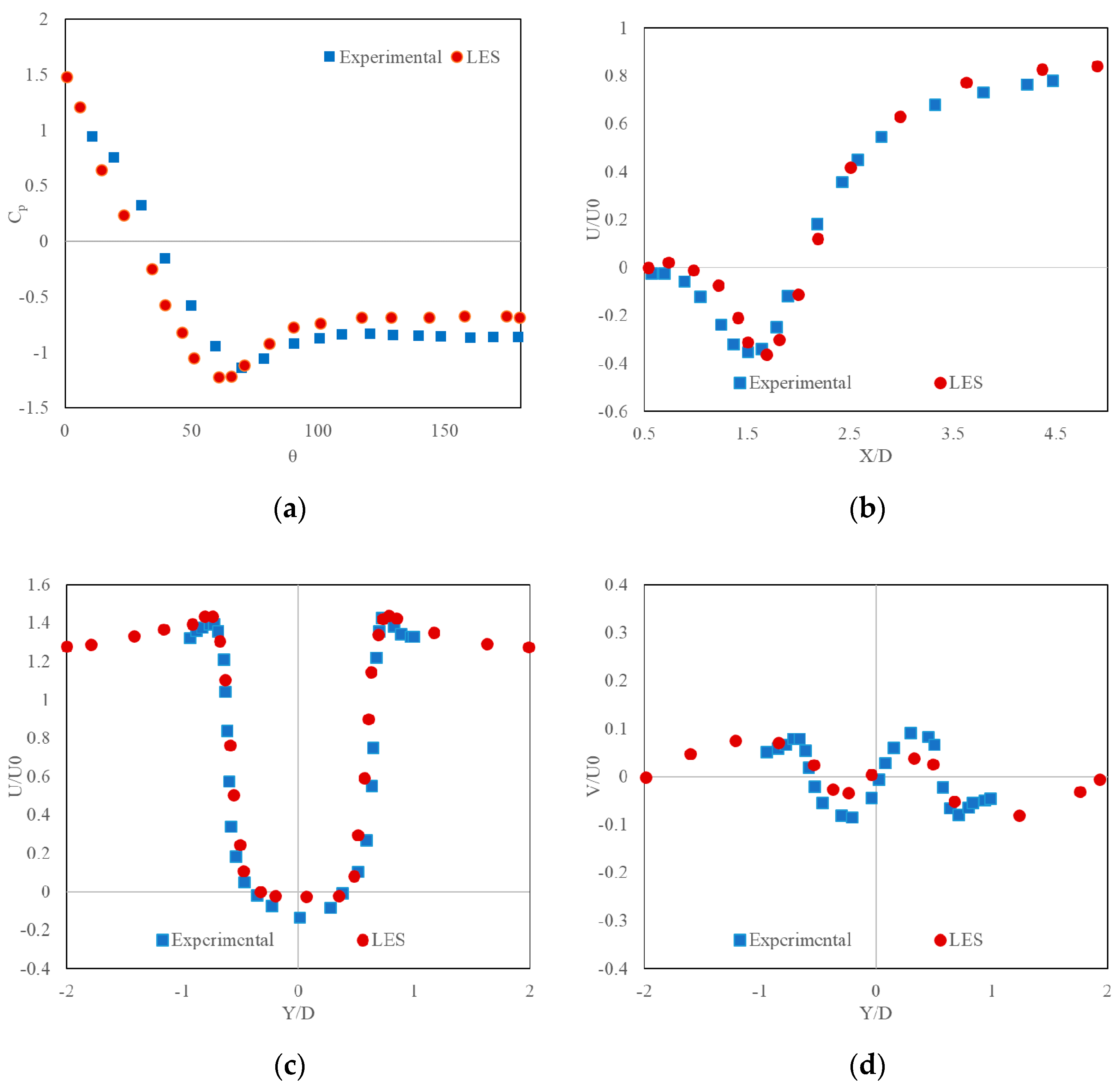
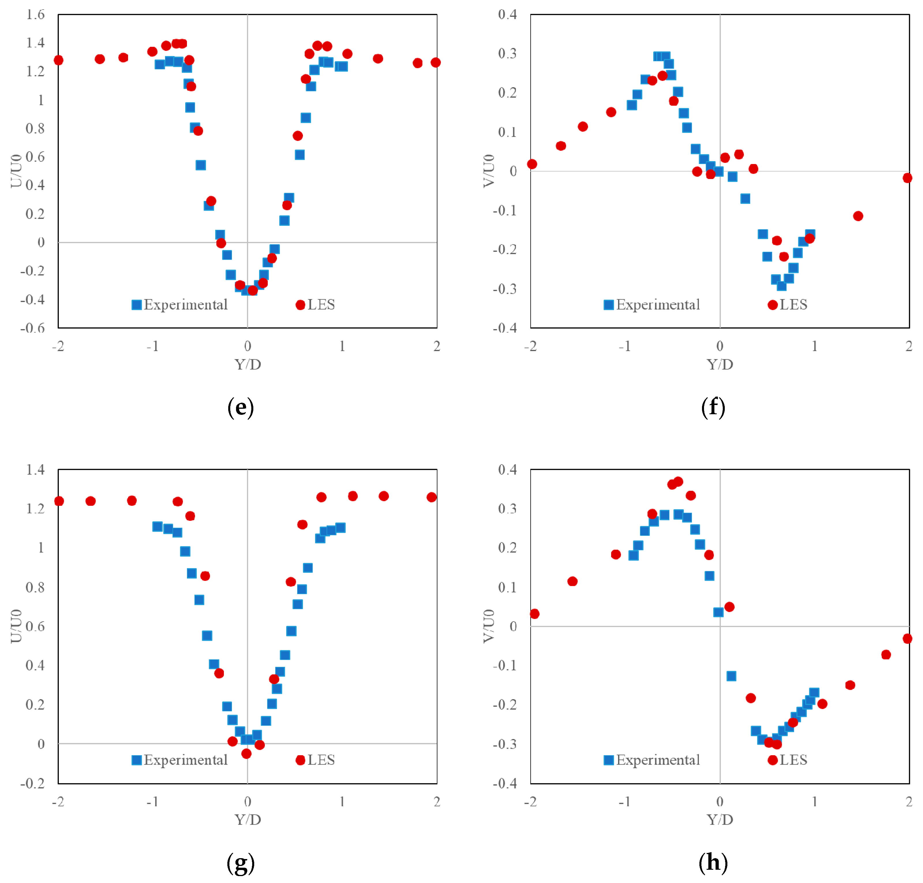
Validation of the LES calculation is done as shown in Figure 1. For this, a turbulent flow over a cylinder at Re = 3900 is adopted to check the validity of the method in predicting the separation of the shear layers in the presence of an obstacle, compared with the experimental data provided by Parnaudeau et al. [13].

Figure 1 indicates acceptable accordance of the LES-based simulation results considering the span-wise periodicity with the experimental data [13].

Proper orthogonal decomposition—developed by Lumley [8] as discussed before—has the capability of extracting the coherent flow structures and ranking the flow modes based on the energy content. In fact, each one of these POD modes contains a share of the total turbulent kinetic energy (TKE) of the flow field. Besides, the modes are ranked based on the energy content. The input of POD is the collected transient field data in the domain of interest by a high-enough number of snapshots. To apply POD on the fluctuating part of velocity, the following decomposition is the starting point of the calculations [14]:

$${\overrightarrow{u}}_i\left({\overrightarrow{x}}_k\right)=\overline{\overrightarrow{u}}\left({\overrightarrow{x}}_k\right)+\overrightarrow{u^{\prime }}\left({\overrightarrow{x}}_k\right)$$

(9)

where ${\overrightarrow{u}}_i\left({\overrightarrow{x}}_k\right)$ represents the velocity field ($i$ = $1$ to $N$), $N$ is the number of snapshots, and ${\overrightarrow{x}}_k$ is the spatial coordinates ($k$ = 1 to $M$), where $M$ is the number of spatial positions. The fluctuating part of the velocity field can be represented by a linear set of space-dependent spatial modes ${\overrightarrow{\varphi }}_j$ and the corresponding purely time-dependent temporal coefficients $a_{ij}$:

$$\overrightarrow{u^{\prime }}\left({\overrightarrow{x}}_k\right)={\displaystyle \sum }_{j=1}^N{a}_{ij}{\overrightarrow{\varphi }}_j\left({\overrightarrow{x}}_k\right)$$

(10)

According to the method of snapshots [15], spatial POD modes and temporal coefficients can be calculated based on the eigenvalues (${\lambda }_j$) and eigenvectors ($e_j$) of the $N\times N$ correlation matrix ($\tilde{C}$) [9]:

$$\tilde{C}=\frac{1}{N}\langle {\overrightarrow{u^{\prime }}}_i · {\overrightarrow{u^{\prime }}}_j\rangle$$

(11)

The temporal coefficients corresponding to the POD modes are calculated as follows:

$$a_{ij}=e_{ij}\sqrt{{\lambda }_{j}N}$$

(12)

The spatial modes satisfy the orthonormality condition as follows:

$$\langle {\overrightarrow{\varphi }}_i · {\overrightarrow{\varphi }}_j\rangle ={\delta }_{ij}$$

(13)

The spatial modes are calculated as follows:

$${\overrightarrow{\varphi }}_j=\frac{1}{{\lambda }_{j}N}{\displaystyle \sum }_{i=1}^N{a}_{ij}{\overrightarrow{u^{\prime }}}_i$$

(14)

Note that each $j^{th}$ mode ${\overrightarrow{\varphi }}_j$ contains a share (${\lambda }_j$) of total turbulent kinetic energy.

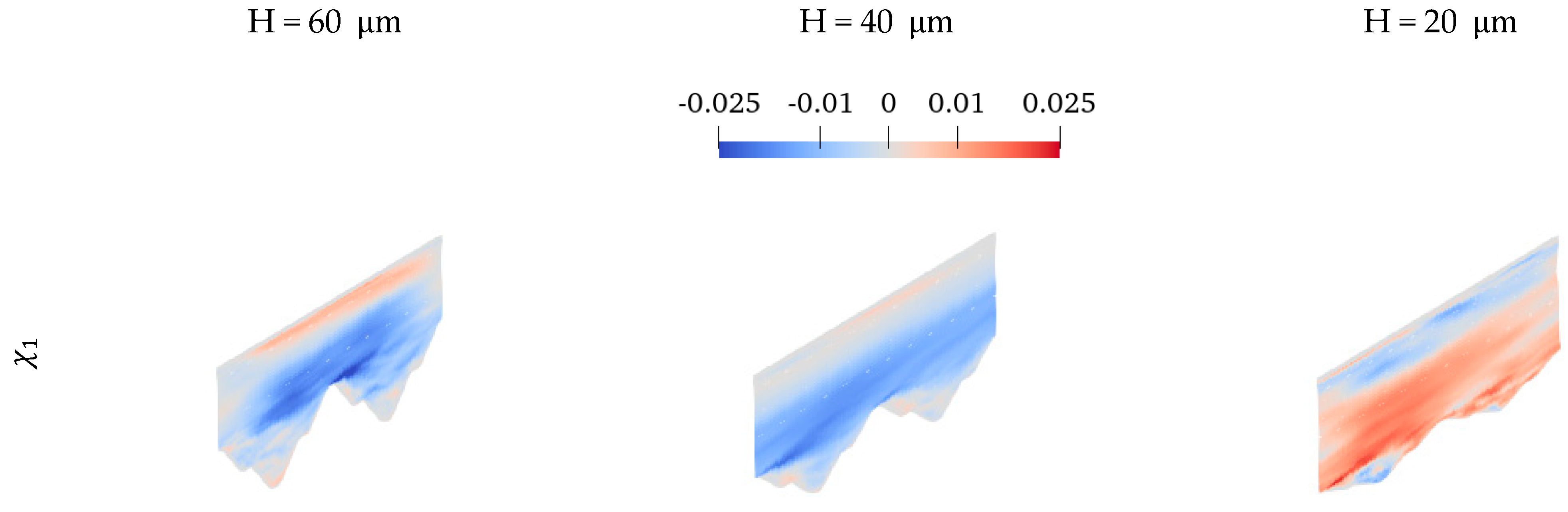
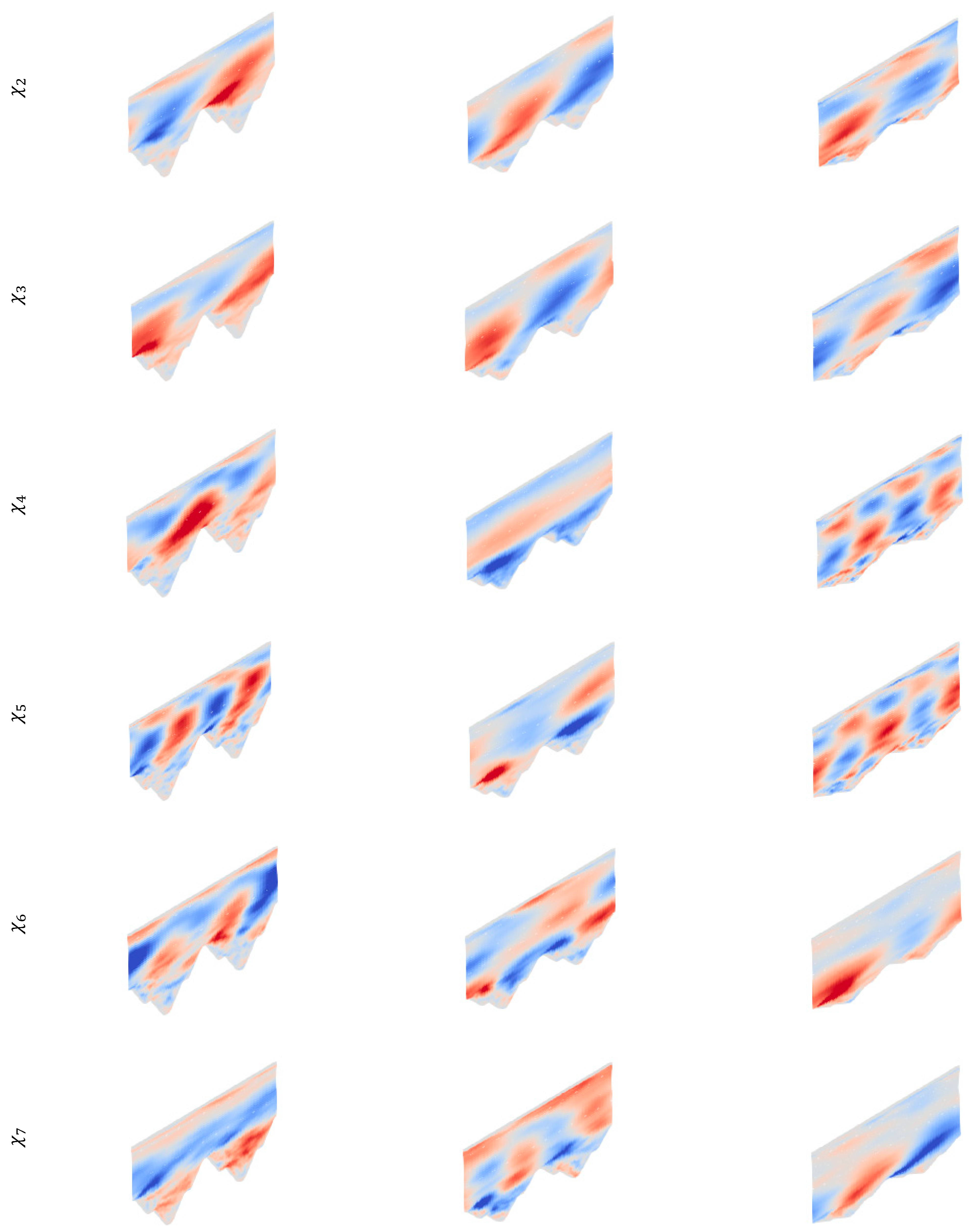
Borée [10] proposed extended proper orthogonal decomposition (EPOD) to conduct correlation analysis between two vector fields or scalar fields, e.g., to study correlation between a flow field and temperature field. To achieve this, the eigenvalue problem for one quantity is solved. Following this, the obtained set of eigenvectors is used to find the modes of the other quantity (in this case, correlation is assessed between the temperature and flow fields). The correlated EPOD modes are hence found by:

$${\chi }_j=\frac{1}{{\lambda }_{j}N}{\displaystyle \sum }_{i=1}^N{a}_{ij}{g}_i^{\prime }$$

(15)

where $g_i^{\prime }$ is the field whose EPOD mode is to be calculated. The correlated field can be found using the EPOD mode [14]:

$${g^{\prime }}_{i,corr}\left({\overrightarrow{x}}_k\right)={\displaystyle \sum }_{j=1}^R{a}_{ij}{\chi }_j\left({\overrightarrow{x}}_k\right)$$

(16)

Additionally, the uncorrelated field can be found by subtraction from the original field:

$${g^{\prime }}_{i,uncorr}\left({\overrightarrow{x}}_k\right)=g^{\prime }{}_{i,orig}\left({\overrightarrow{x}}_k\right)-g^{\prime }{}_{i,corr}\left({\overrightarrow{x}}_k\right)$$

(17)

3. Model Description

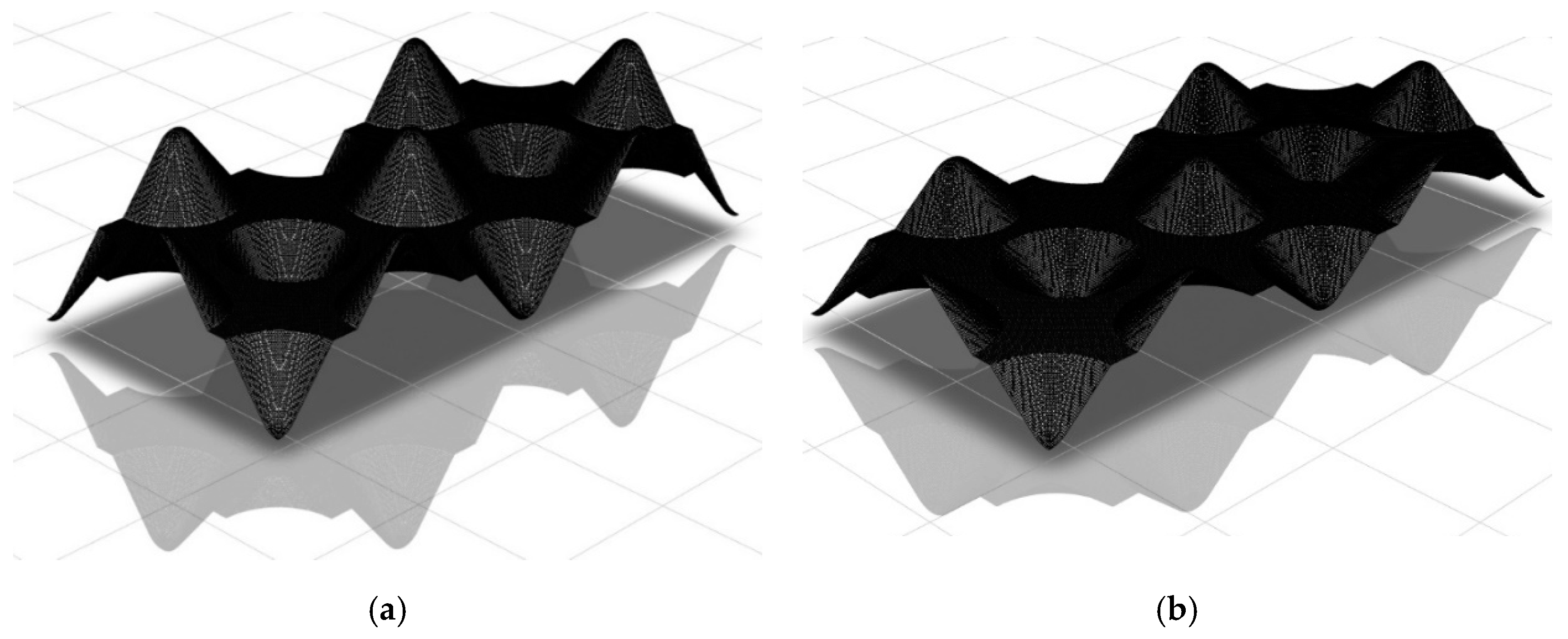
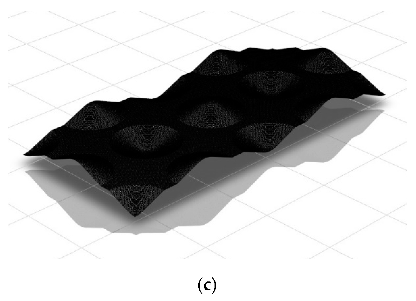
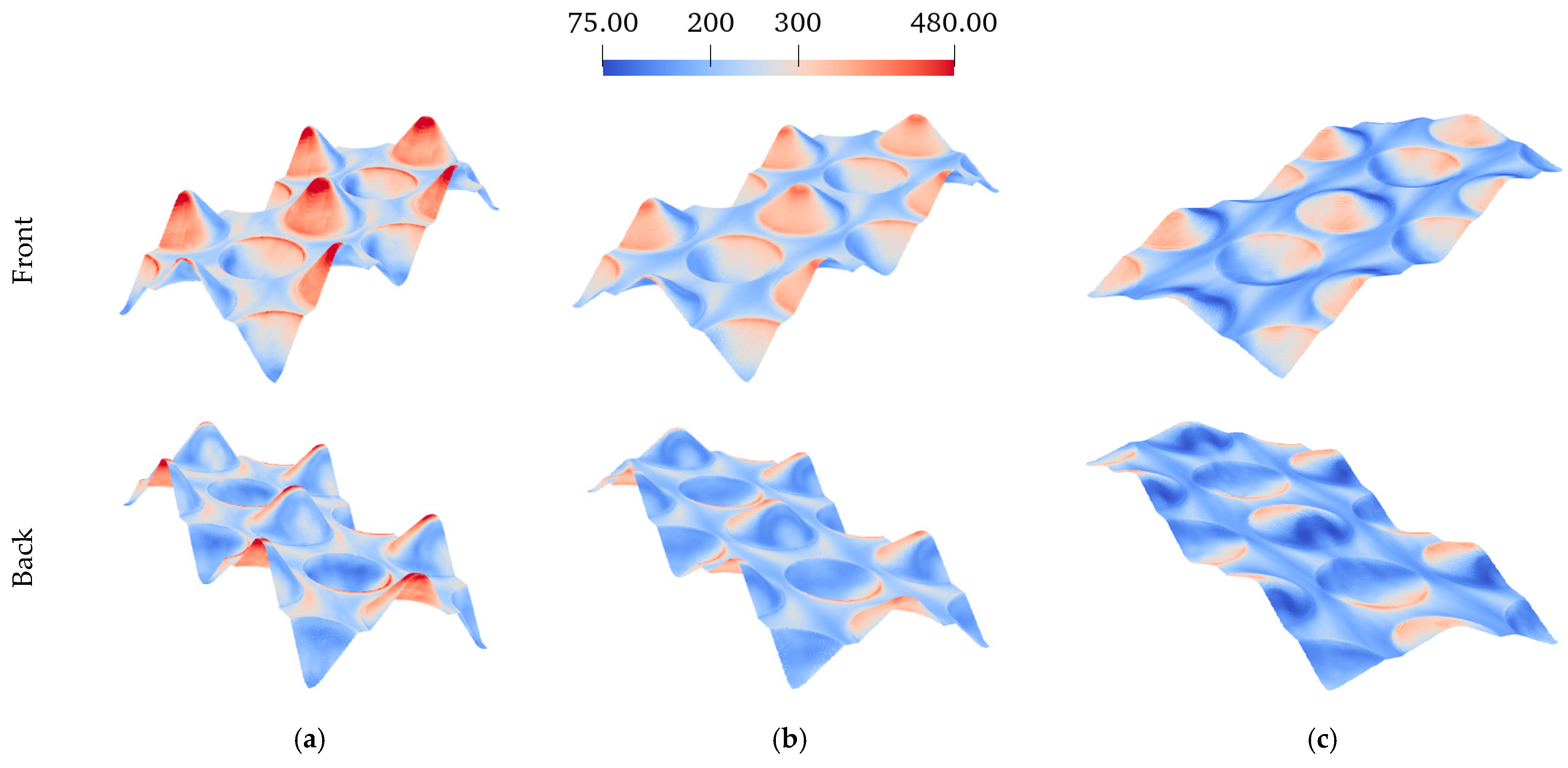
Based on the roughness topology provided in [5] corresponding to a part manufactured by direct metal laser sintering, the roughness model for the current POD/EPOD-based study is considered as cone-shaped peaks/valleys at three levels of heights (at each level, the roughness elements are of the same height) with a fixed base diameter and regular placement of the roughness elements on the surface as shown in Figure 2, Figure 3 and Figure 4. It must be noted that the randomness of geometrical parameters corresponding to the roughness elements and their placement, which is naturally arising in the real surface roughness topology, is not considered in the model. In fact, the model takes into account the dominant roughness elements as cone-shaped peaks/valleys to extract the dominant flow mechanisms governing the heat transfer from the rough surface. The investigated cases in this study include roughness heights of 20 $\mathsf{\mu }\mathrm{m}$, 40 $\mathsf{\mu }\mathrm{m}$, and 60 $\mathsf{\mu }\mathrm{m},$ corresponding to a height-to-base diameter ratio of $H/D=0.175, 0.350,$ and $0.525$, respectively. 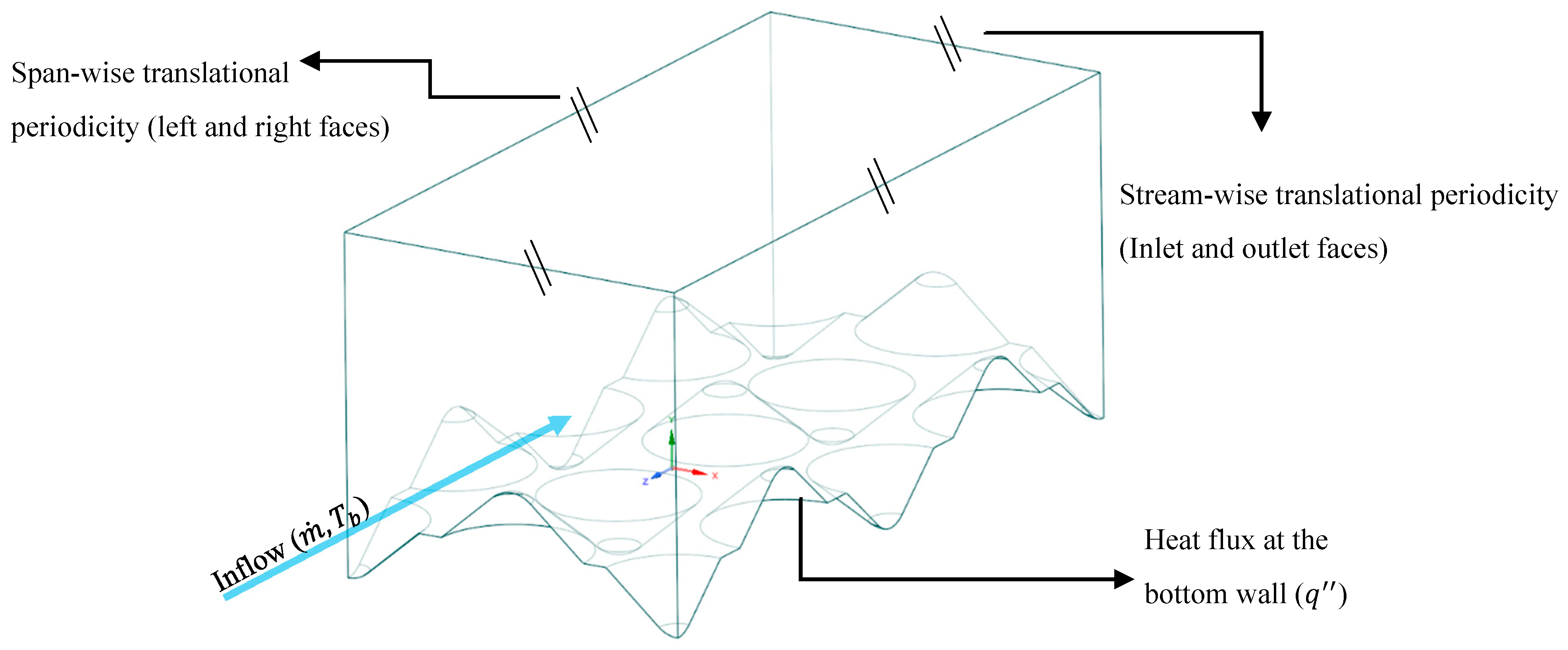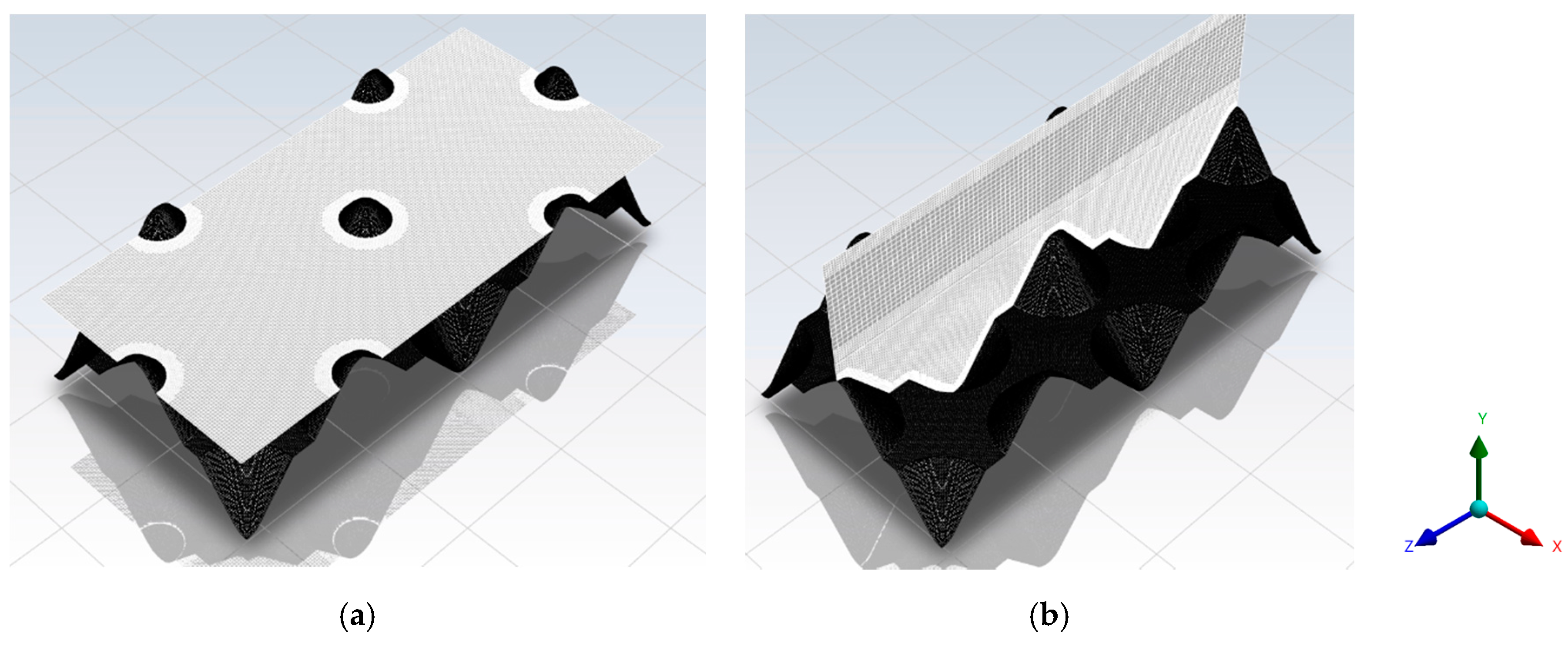The span-wise and stream-wise distance between the cone peaks in the cone-shaped roughness model are assumed as 127.8 $\mathsf{\mu }\mathrm{m}$ and 134.0 $\mathsf{\mu }\mathrm{m}$, respectively. The same is used for the stream-wise and span-wise distance between valleys. The computational domain and the applied boundary conditions are provided in Figure 2, and the three levels of roughness are illustrated in Figure 4.

As shown in Figure 2, stream-wise and span-wise periodicity is considered for the computational domain, and the mass flow rate ($\dot{\mathrm{m}}$) in the stream-wise direction is specified along Z, with a specific inflow bulk temperature (${\mathrm{T}}_{\mathrm{b}}=363.15 \mathrm{K}$). The bottom wall is subject to constant heat flux (${10}^5\mathrm{W}/{\mathrm{m}}^2$). The top wall is taken to be adiabatic with a no-slip condition. The mass flow rate over the periodic domain corresponds to Re = 1.26 $\times {10}^4$, where the Re is calculated based on the height of the periodic domain [7].

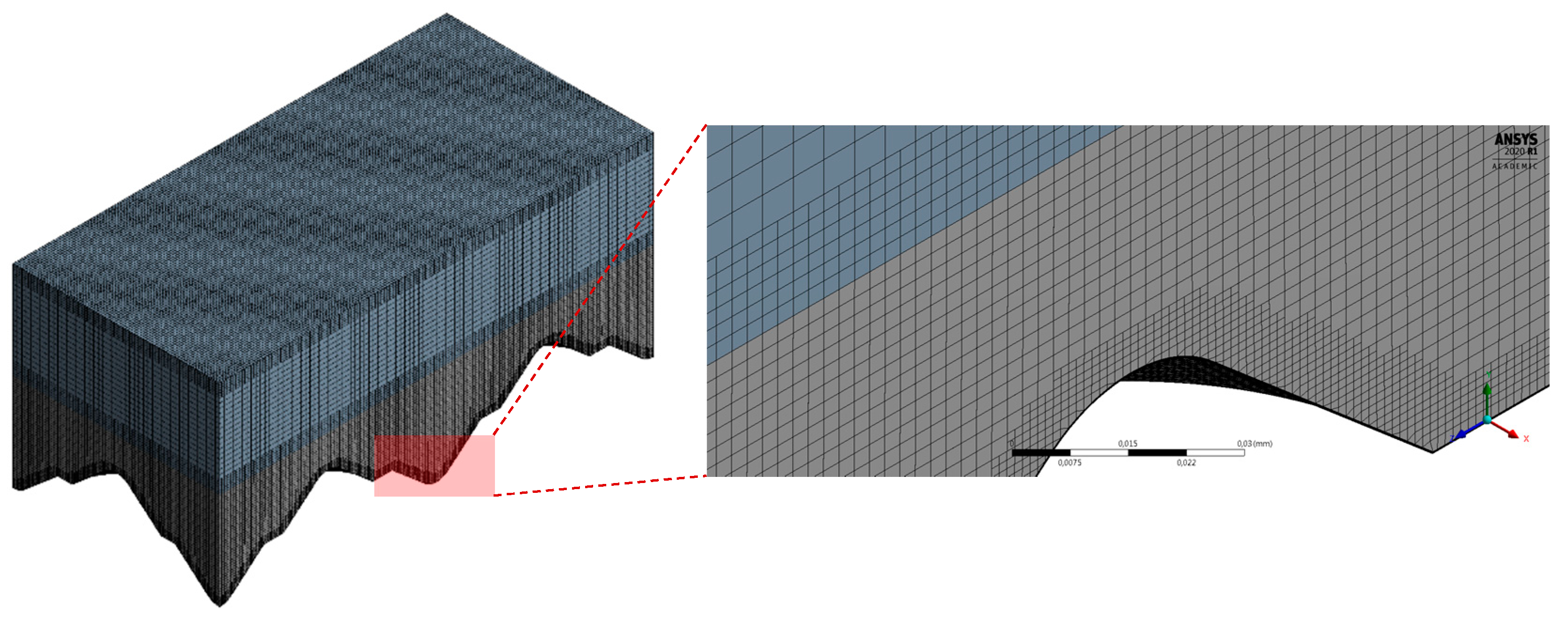
To give an overview of the generated mesh and corresponding resolution, the three-dimensional mesh for the periodic domain studying the roughness effect for the mid-level of roughness is shown in Figure 3. Cut-Cell Meshing technology is used in ANSYS-Meshing in order to achieve the desired near-wall mesh refinement with close-to-one aspect ratios. For the illustrated mesh, the total number of cells is $2.3\times {10}^{+6}$ and the near-wall mesh resolution is $\widetilde{∆x^{+}}\approx \widetilde{∆z^{+}}\approx$ 14.2 and $\widetilde{∆y^{+}}\approx$ 0.20, where the provided values for $\widetilde{∆x^{+}}$, $\widetilde{∆y^{+}}$, and $\widetilde{∆z^{+}}$ are the facet maximum values representing the stream-wise, wall-normal, and span-wise resolutions, respectively. In more detail, $∆y^{+}$ represents the non-dimensional wall distance for a wall-bounded flow defined as $∆y^{+}\equiv 2\rho u_{\tau }y/\mu$, where $\rho$ is the fluid density, $u_{\tau }$ is the friction velocity at the nearest wall, y is the distance to the nearest wall, and $\mu$ is the local dynamic viscosity of the fluid. Moreover, $\widetilde{∆x^{+}} \mathrm{and} \widetilde{∆y^{+}}$ are calculated as the square root of the multiplication of $y^{+}$ and face area magnitude, i.e., the magnitude of the face area vector for the non-internal faces, divided by the cell wall distance, i.e., the distribution of the normal distance of each cell centroid from the wall boundaries [16]. It is noteworthy that the difference in the resolution report of the wall-normal and stream-wise directions is due to the very thin inflation layers.

Menter’s SST k-ω [17] is conducted as a precursor RANS simulation to identify the suitable mesh resolution, and once this is done, the time step size is estimated. The bounded second-order implicit method is used for the transient formulation, and the iterative time advancement method is applied in the entire calculation. The LES calculations are initialized by the converged RANS steady solution with a small time step size corresponding to Courant numbers as low as 0.1, and a high number of iterations per time step (as high as 100). Following this, the time step size is ramped up to CFL $\approx$ 10, and the number of iterations per time step is also reduced to 20. During this time, the domain is washed at least once. The required time duration is roughly determined by the channel length and flow characteristic velocity. Finally, the time step size is ramped down to CFL around one up to the statistically averageable state. Once this is reached, the snapshots containing instantaneous thermal/flow fields are exported. The final time step used in this procedure is $5\times {10}^{-8} \mathrm{s}$, and the maximum No. of iterations per time step is 100 at the beginning and 20 when exporting snapshots. The total No. of time steps for exporting snapshots is 12,000 with 4 as the data exporting frequency. The sub-grid scale model is the WALE model with $C_w$ = 0.325. The SIMPLE scheme is used for pressure-velocity coupling. The spatial discretization of the gradient, pressure, momentum, and energy is done by least squares cell-based, second order, bounded central differencing, and second order upwind, respectively.

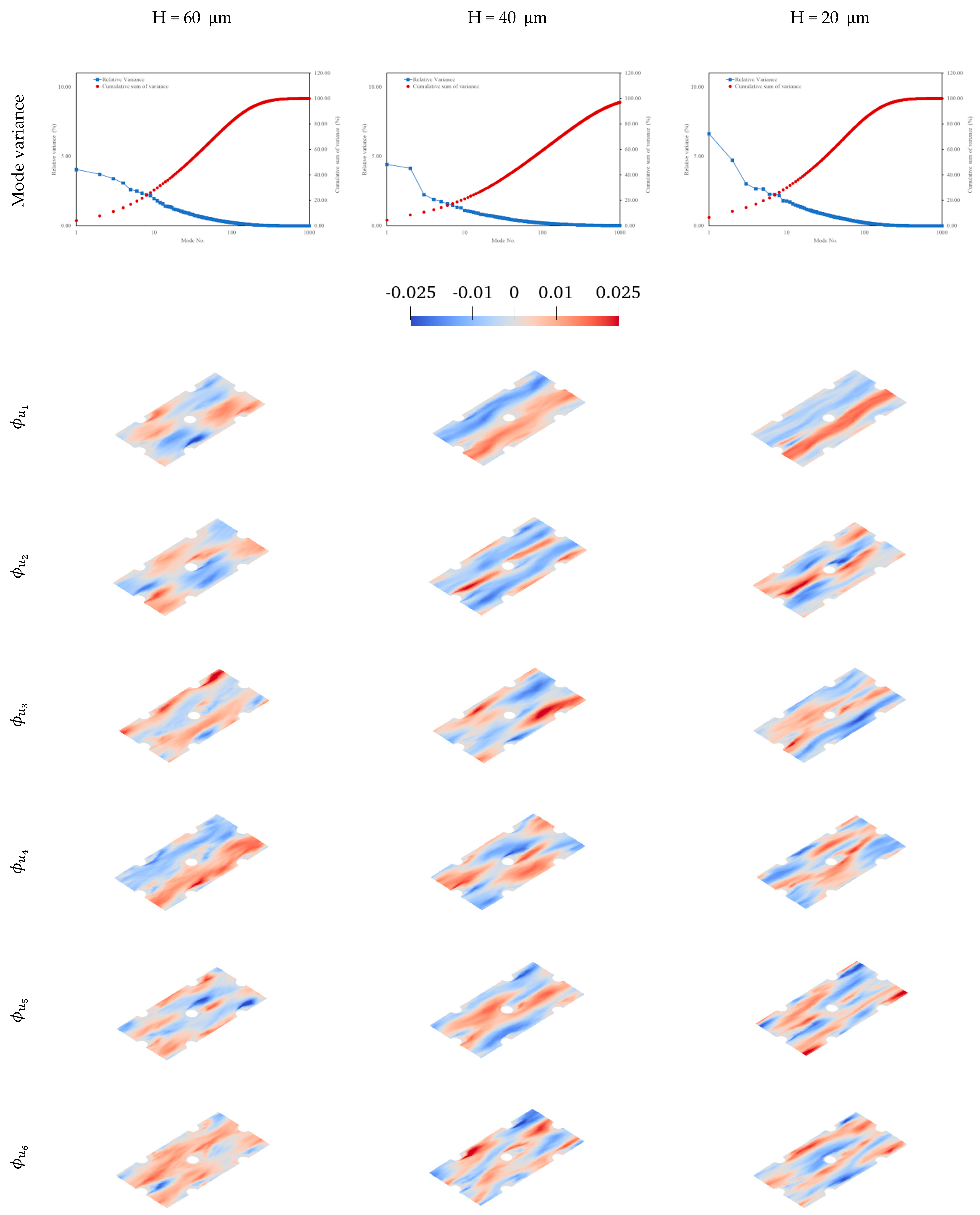
For the modal decomposition analysis, the snapshots of the flow/thermal fields are reported on the horizontal and wall-normal stream-wise planes as illustrated in Figure 5. The horizontal plane in all cases is located at $Y=2/3H$, where $H$ is the peak height, and the wall-normal plane is located at the middle of the periodic domain along the X-axis at X = 0 as shown in the figure. In the present study, the shown 2D planes are used to export the flow/thermal data to conduct the modal decomposition analysis at a reduced computational cost in terms of input files. The limits of this approach must be considered; specifically, the mixing between the flow mechanisms observed in these two planes and the absence of the out-of-plane velocity component affects the analyses. Modal decomposition study of 2D planes extracted from the fluid domain has been used in numerous studies (see [18,19,20]) According to Meyer et al. 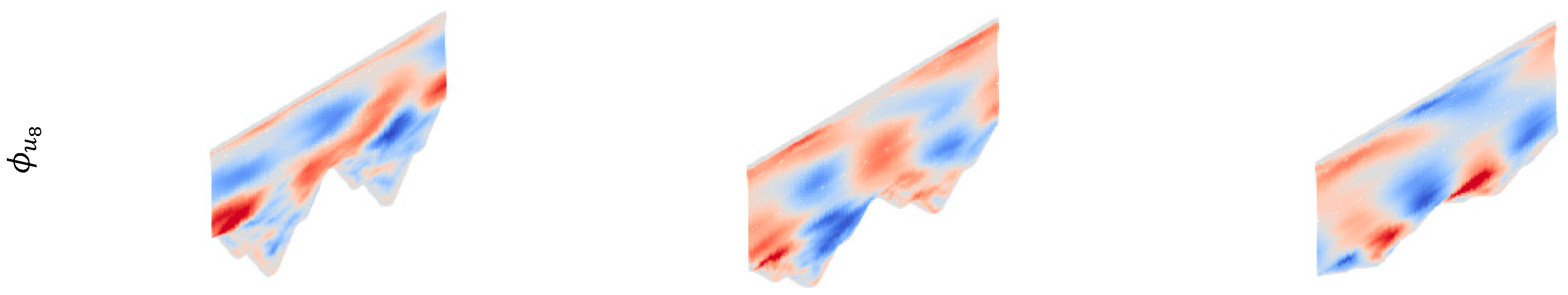[20], POD study conducted on planes would agree well with the “true” three-dimensional analysis as long as the plane contains the important phenomena in the flow. Accordingly, flow/thermal snapshots in this paper are exported on a horizontally mounted plane in addition to the wall-normal stream-wise plane so as to consider the span-wise mixing effect in the horizontal plane that is not observed in the stream-wise wall-normal plane.

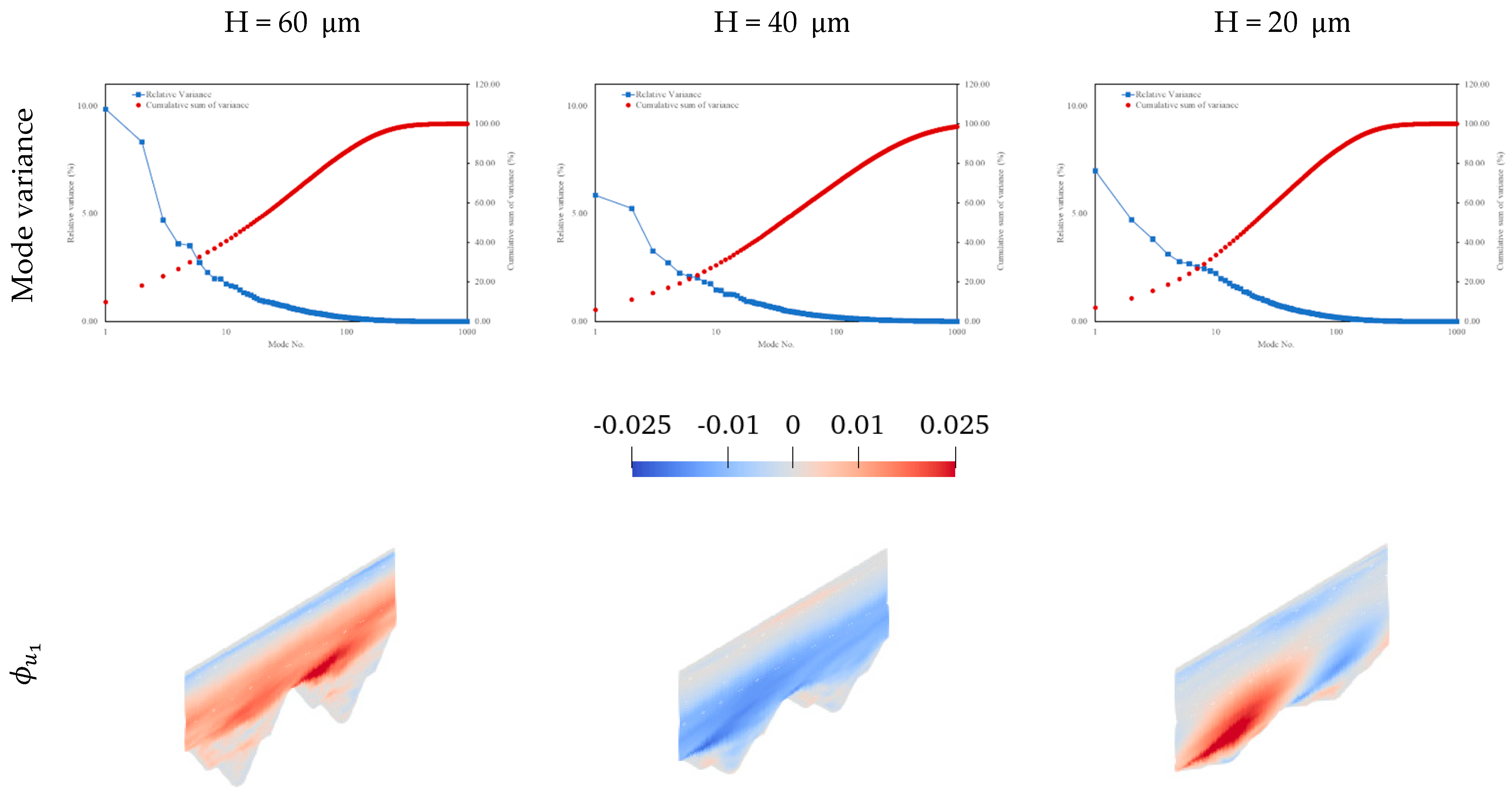
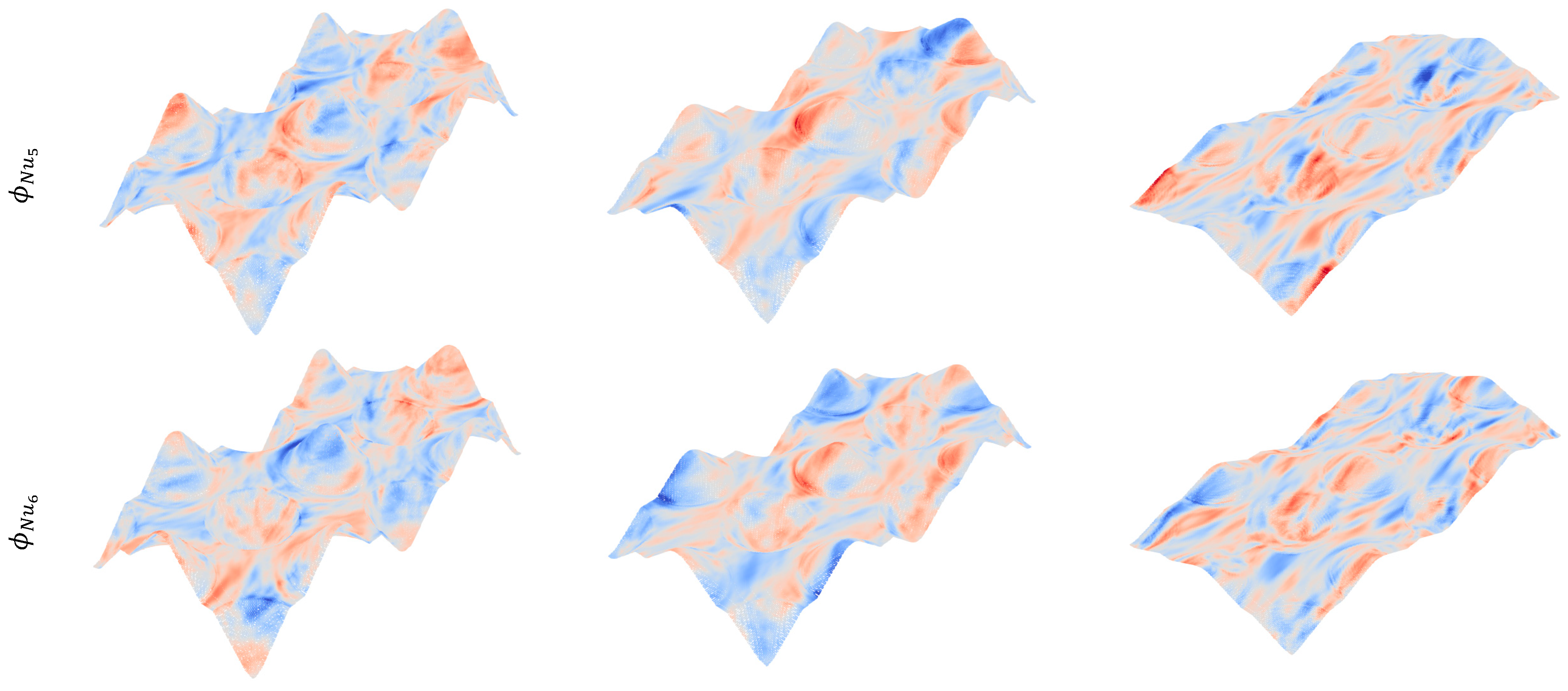
4. Results and Discussions

4.1. Modal Decomposition Analysis of the Velocity Field on the Rough Surface Model

The TKE-ranked POD modes of the stream-wise velocity in the wall-normal plane for all three levels of roughness heights are shown in Figure 6. The modes corresponding to the high level of roughness indicate that among the low-order energetic flow modes, the so called Kelvin–Helmholtz instability [21] is observed (see modes No. 2, 3, 4, and 5). Due to the appearance among the low-order/high-energy POD modes, this instability is recognized as the dominant flow mechanism in stream-wise wall-normal planes, which is promoted and intensified by the peaks of the roughness profile as the wall-attached obstacles. In addition, the other point is the existence of strong active flow fluctuations in the core flow as well as in the near-wall flow as a result of the strengthened fluctuations by the high-rise peaks in the case of a high level of roughness. In spite of the positive aspects, the negative point for thermal transport is the minimal engagement of valleys in terms of the absence of strong velocity fluctuating structures due to the flow trap effect in the case of high roughness. This becomes clear when comparing the mode shapes with the corresponding ones at the low level of roughness height. This effect comes from the dead fluctuation zone in the valleys. To verify if the valleys are involved in thermally important modes, the EPOD modes of this case are discussed in the next sections. The POD modes of velocity corresponding to the medium level of roughness provided in Figure 6 show the same flow mechanism as the dominant/energetic as for the high roughness level. However, even among the energetic modes, a higher engagement of valleys in terms of strong flow fluctuations is observed. Active fluctuations in this area are important to avoid local dead areas/hot spots. The other point is that in the medium roughness level, a balance is observed between the strong Kelvin–Helmholtz structures and the engagement of valleys. This is in contrast to the case with the low level of roughness as shown later. Finally, when comparing the energy distribution and mode shapes of velocity eigenmodes at the low level of roughness height with the high roughness case, the first inferred point is the similar energy distribution and flow mechanism in the stream-wise wall-normal plane. In fact, the same flow mechanism is introduced by the wall-attached roughness structures. However, the main difference is where the active strong fluctuations take place. In this regard, valleys are more engaged so that the dead fluctuation zone is avoided. The other point is the shift of the coherent flow modes of the low level of roughness to the near-wall area, while the corresponding flow modes at the high level of roughness show strong fluctuating structures in the core area as well as near the wall. This is important to achieve core flow-near wall flow mixing.

The POD modes illustrated in Figure 7 are the TKE-ranked POD modes for the stream-wise velocity in the horizontal plane. As shown in this figure for the high level of roughness height, according to the first few energetic modes, von Kármán instability is observed among the dominant flow mechanisms in the horizontal plane induced by the peaks of surface roughness elements. The von Kármán instability is clearer for a high level of roughness in modes No. 1, 2, 5, 6, 7, and 8. This mechanism is responsible for the intensification of span-wise flow mixing. One point is that this flow mechanism is exclusively produced by the peaks in the roughness profile, and the valleys do not contribute to it. Moreover, due to the desired flow mixing by this mechanism, it is beneficial for thermal transport. This is the other reason behind the beneficial effects of peaks in heat transfer. Finally, it is worth mentioning that this flow mixing is active for a wider wall-normal distance in the case of high-rise peaks compared to the low level of roughness. The mode shapes in this plane at a medium and low level of roughness indicate that the von Kármán mechanism is still observed at a low level of surface element roughness; however, at the low level of roughness height, it is observed in more streak-like shapes in the 2D plane. The fact that the dominance of this flow mechanism is lost is also observed in terms of losing the coherence as shown in the energy distribution diagram, where the trend of the energy distribution shows a strict decreasing behavior. The other point is that aside from the weaker mixing, in this case, the lower height of the peaks responsible for this flow mechanism reduces the overall wall-normal distance where this mixing mechanism exists, which is acting against the roughness-induced heat transfer enhancement.

The reason behind having two different dominant flow mechanisms in the two studied planes, i.e., stream-wise wall normal and horizontal planes, lies in the fact that in the wall-normal planes, flow is taking place over ‘wall-attached obstacles’. In accordance with literature [21], for the case of flow over an obstacle with no gap between the obstacle and wall, i.e., fully wall-attached obstacle, the dominant flow mechanism is Kelvin-Helmholtz promoted by the obstacle. This is responsible for small-scale flow structures in the near-wall region promoting heat transfer from the surface. On the other hand, the low-order energetic flow modes in the horizontal plane indicate a different flow mechanism, i.e., von Kármán instability promoted by the peaks of the roughness elements. This is very similar to the simplified case of having pin-shaped obstacles attached to the walls, where von Kármán instability is generated by the pin structures.

The EPOD modes representing thermally importance-based ranked flow modes are provided in Figure 8. According to the mode shapes corresponding to the high level of roughness, the EPOD modes verify the fact that the active/strong fluctuating structures are mainly introduced by peaks, and the valleys in the case of a high roughness level play a minimal role in thermal transport. The other point inferred from the EPOD modes is the similarity of the mode topologies to the energetic POD modes. This shows the importance of the energetic flow structures in heat transfer in the analyzed 2D stream-wise wall normal planes. The EPOD modes in Figure 8 corresponding to the medium level of roughness show the thermal importance of the large-scale Kelvin–Helmholtz-induced structures followed by small-scale structures distributed in the entire domain including valleys. This verifies the thermal importance of valley-involving flow modes, which is acting against the flow trap effect in these areas. With the reduction of the large-scale flow structures in the case of the low level of roughness, there is a change in the rank of thermally important flow modes compared to the energy-based ranked modes. In fact, the large-scale Kelvin–Helmholtz-induced structures still appear among the first few modes, but above them, the small-scale structures active all over the domain gain thermal importance. In more detail, comparison between Figure 6 and Figure 8 indicates that for the high level of roughness, the same mode topologies appear as the first few energetic POD modes and thermally-important EPOD modes. However, when the same comparison is made for the low level of roughness, it is observed that the first few large-scale POD modes that appear as the most energetic among the TKE-ranked modes come after some small-scale flow structures among the thermally important EPOD modes. This is attributed to the fact that the energetic POD modes corresponding to the Kelvin–Helmholtz mechanism at a low level of roughness lose their thermal importance compared to the high level of roughness. In addition to the mentioned points, the engagement of valleys in the thermally important modes can also be observed in this figure.

4.2. Modal Decomposition of the Transient Nusselt Field on the Rough Surface

Prior to applying modal decomposition study on the Nu field, the temporal mean of the local Nusselt on the heated wall is shown in Figure 9. The local Nu is calculated by $\mathrm{Nu}=\left({\mathrm{hD}}_{\mathrm{h}}\right)/{\mathrm{k}}_{\mathrm{f}},$ where $\mathrm{h}$,${ \mathrm{D}}_{\mathrm{h}}$, and ${\mathrm{k}}_{\mathrm{f}}$ represent the convective heat transfer coefficient, hydraulic diameter, and fluid thermal conductivity, respectively. Besides, $\mathrm{h}$ is calculated as $\mathrm{h} = {\mathrm{q}}^{″}/\left({\mathrm{T}}_{\mathrm{w}}-{\mathrm{T}}_{\mathrm{b}}\right)$, where ${\mathrm{q}}^{″}$, ${\mathrm{T}}_{\mathrm{w}}$, and ${\mathrm{T}}_{\mathrm{b}}$ represent the heat flux, wall temperature, and fluid bulk temperature, respectively. As illustrated in this figure, one plus point of the high-rise roughness peaks is observed as the impingement of the coolant on it. This effect is stronger at a higher level of heights. However, the negative aspect is also observed on the rear side of the peaks in terms of considerably low-Nu areas.

POD is applied on the Nu field over the rough surface to evaluate the footprint of the flow and thermal fields on the heat transfer characteristics of the roughness model. Figure 10 shows the mode variance distributions and spatial POD modes of the Nu field on the surface at the three levels of roughness heights.

Comparison between the spatial mode shapes of Nu on the rough surface between the low and high levels of roughness shows a streakier pattern of Nu eigenmodes when tending from the high level of roughness toward the more smooth surface. In fact, the dominant-high-variance Nu eigenmodes are mainly formed by the streak structures of low/high Nu elongated in the stream-wise direction. Note that even at the roughness height of 20 μm, the span-wise von Kármán mixing still exists, and the structure is not fully streaky. In fact, in the case of a fully smooth surface, the role of the abovementioned small-scale flow structures in the near-wall region is absent. In such cases, the large-scale sweeps/ejections in the system would govern the thermal response of the surface [21], and the small-scale near-wall vortices are almost absent due to the absence of rough elements responsible for such flow structures. Therefore, in such cases, the Nu eigenmodes of streak shapes are expected. However, in all of our cases, the mentioned flow instabilities cause near-wall vortices, but as mentioned, with a tendency toward a smooth surface, the more streak-like spatial mode shapes of Nu are observed. From the comparison between Nu mode shapes of the high and low levels of roughness (here $H=60 \mathsf{\mu }\mathrm{m} \mathrm{and} 20 \mathsf{\mu }\mathrm{m}$, respectively), it is inferred that in contrast with the streaky shapes of the POD modes of Nu at the low level of roughness, the pattern is strongly distorted with the increase of the roughness height. This is attributed to the intensification of span-wise mixing as a result of intensifying von Kármán induced by the high-rise peaks on the surface.

Aside from the mode shapes, the mode variance distributions for the Nu numbers verify the intensification of the thermal role of span-wise mixing with the increase of the roughness height. In fact, with the increase of the roughness height to $H=60 \mathsf{\mu }\mathrm{m}$, the pattern of the Nu mode variance distribution (see Figure 10) becomes very similar to the mode variance distribution pattern of the corresponding height for the flow modes in the horizontal plane, which is dominated by the von Kármán mechanism (see Figure 7). This is attributed to the more dominant role of span-wise mixing caused by von Kármán instability with the increase of height level of high-rise peaks.

From the modal analysis viewpoint, it was indicated how the peaks intensify both observed flow mechanisms, how the valleys do not participate in the von Kármán mechanism, and how valleys can cause a dead fluctuation zone due to the flow trap effect. Accordingly, it seems necessary to provide proposals on how to manipulate additively manufactured surface roughness topology for the sake of thermal transport considerations. To be pragmatic, the recommendation for the surface roughness control either during printing or by post-printing surface treatment is to consider the average roughness height-to-base-diameter ratio for a fair sample area on the rough surface as the surface design parameter. This is, because the mid-level of this parameter can balance the intensified Kelvin–Helmholtz mechanism, the von Kármán-induced mixing by peaks, and the reduction of dead fluctuation zones in valleys. The actual thermal response in terms of the maximum surface temperature and surface Nusselt number are provided in Figure 11. It is observed in this figure that the high level of the height-to-base-diameter causes local hot spots, and the close-to-perfectly-smooth surface would lack the desired flow mixing caused by the natural roughness of the surface. As indicated in this figure, the increase of the roughness height leads to an increase of the averaged Nu on the rough surface. However, due to the illustrated dead fluctuating zones in the valleys in the case of the high level of roughness, this increase in Nu is not seen in terms of a maximum temperature reduction. In other words, the dead fluctuating zones cause thermal performance saturation.

5. Conclusions

The conducted study investigated thermo-hydraulic behavior of a three-dimensional model representing a natural roughness profile observed in additive manufacturing. The surface roughness model is assumed as cone-shaped elements at three levels of height and regular placement of roughness elements as the major roughness structures playing a role in the flow/thermal performance of the system. LES was used to provide detailed flow/thermal fields in the transient form. The transient data were imported into modal decomposition analyses, i.e., POD/EPOD, to extract the energetic and thermally important flow modes. The obtained results indicated that in general, the flow mechanisms responsible for thermal transport are von Kármán in horizontal planes and Kelvin–Helmholtz in stream-wise wall-normal planes. A comparison was made between the POD/EPOD results of the three levels of roughness. Minimization of the dead areas corresponding to hot spots in the micro-scale roughness profile is of crucial importance. This is because regardless of the macro-scale flow mixing promoters, the high number of local dead fluctuation zones containing trapped flow acting as an insulator due to the lower thermal conductivity of common coolants in liquid/air cooling-based devices would reduce the overall performance. This is where roughness can act against the heat transfer purpose. Based on this, the surface roughness manipulation must act in a way that this effect is minimized. The recommendation is to consider the average height-to-base-diameter ratio as the thermal consideration along with the arithmetic average roughness for the design of heat exchangers to be realized by additive manufacturing. While the high ratio roughness benefits from the plus points induced by the high-rise peaks, the thermally inactive dead valleys have a negative effect. At the mid values of this ratio, the high number of local dead areas is reduced, and it still benefits from the shown mixing mechanisms by peaks. It is noteworthy that in the case of a fully smooth surface, the role of von Kármán-induced mixing in horizontal planes and Kelvin–Helmholtz mixing in stream-wise wall normal planes fade. In this case, the transport would be on the shoulder of sweep/ejection mechanisms taking place on smooth surfaces. Finally, it must be noted that the surface roughness model in this work is based on cone-shaped peak/valley structures, so that compared to the real rough surface, the random geometrical parameters of each roughness element and the randomness of placement of roughness elements are absent. Future work is to be conducted on a real 3D-printed surface roughness sample, so that the CFD domain is reconstructed using the point cloud extracted by computed tomography scanning of the rough surface, and the instantaneous flow/thermal fields to be imported into the established POD/EPOD study.

References

1. ASTM International. ASTM52900-15 Standard Terminology for Additive Manufacturing—General Principles—Terminology; ASTM International: West Conshohocken, PA, USA, 2015; Volume 3, p. 5. [Google Scholar]
2. Kaur, I.; Singh, P. State-of-the-art in heat exchanger additive manufacturing. Int. J. Heat Mass Transf. 2021, 178, 121600. [Google Scholar] [CrossRef]
3. Dugbenoo, E.; Arif, M.F.; Wardle, B.L.; Kumar, S. Enhanced Bonding via Additive Manufacturing-Enabled Surface Tailoring of 3D Printed Continuous-Fiber Composites. Adv. Eng. Mater. 2018, 20, 1800691. [Google Scholar] [CrossRef]
4. Dixit, T.; Nithiarasu, P.; Kumar, S. Numerical evaluation of additively manufactured lattice architectures for heat sink applications. Int. J. Therm. Sci. 2020, 159, 106607. [Google Scholar] [CrossRef]
5. Stimpson, C.K.; Snyder, J.C.; Thole, K.A.; Mongillo, D. Roughness Effects on Flow and Heat Transfer for Additively Manufactured Channels. J. Turbomach. 2016, 138, 051008. [Google Scholar] [CrossRef]
6. Isaev, S.; Schelchkov, A.; Leontiev, A.; Gortyshov, Y.F.; Baranov, P.; Popov, I. Vortex heat transfer enhancement in the narrow plane-parallel channel with the oval-trench dimple of fixed depth and spot area. Int. J. Heat Mass Transf. 2017, 109, 40–62. [Google Scholar] [CrossRef]
7. Turnow, J.; Kornev, N.; Zhdanov, V.; Hassel, E. Flow structures and heat transfer on dimples in a staggered arrangement. Int. J. Heat Fluid Flow 2012, 35, 168–175. [Google Scholar] [CrossRef]
8. Lumley, J.L. The structure of inhomogeneous turbulent flows. In Atmospheric Turbulence and Radio wave Propagation; Publishing House Nauka: Moscow, Russia, 1967; pp. 166–176. [Google Scholar]
9. Eßl, W.; Pfeiler, C.; Reiss, G.; Ecker, W.; Riener, C.K.; Angeli, G. LES-VOF simulation and POD Analysis of the Gas-Jet Wiping Process in Continuous Galvanizing Lines. Steel Res. Int. 2017, 89, 1700362. [Google Scholar] [CrossRef]
10. Borée, J. Extended proper orthogonal decomposition: A tool to analyse correlated events in turbulent flows. Exp. Fluids 2003, 35, 188–192. [Google Scholar] [CrossRef]
11. Lohrasbi, S.; Hammer, R.; Eßl, W.; Reiss, G.; Defregger, S.; Sanz, W. A modification to extended proper orthogonal decomposition-based correlation analysis: The spatial consideration. Int. J. Heat Mass Transf. 2021, 175, 121065. [Google Scholar] [CrossRef]
12. ANSYS. ANSYS Fluent User’s Guide, Release 19.0; ANSYS: Canonsburg, PA, USA, 2018. [Google Scholar]
13. Parnaudeau, P.; Carlier, J.; Heitz, D.; Lamballais, E. Experimental and numerical studies of the flow over a circular cylinder at Reynolds number 3900. Phys. Fluids 2008, 20, 085101. [Google Scholar] [CrossRef] [Green Version]
14. Stöhr, M.; Sadanandan, R.; Meier, W. Phase-resolved characterization of vortex–flame interaction in a turbulent swirl flame. Exp. Fluids 2011, 51, 1153–1167. [Google Scholar] [CrossRef] [Green Version]
15. Sirovich, L. Chaotic dynamics of coherent structures. Phys. D Nonlinear Phenom. 1989, 37, 126–145. [Google Scholar] [CrossRef]
16. Gerasimov, A. Quick Guide to Setting Up LES-Type Simulations; ANSYS Sweden AB: Goteborg, Sweden, 2016. [Google Scholar]
17. Menter, F. Zonal Two Equation k-w Turbulence Models for Aerodynamic Flows. AIAA 1993. [Google Scholar] [CrossRef]
18. Mallor, F.; Raiola, M.; Vila, C.S.; Örlü, R.; Discetti, S.; Ianiro, A. Modal decomposition of flow fields and convective heat transfer maps: An application to wall-proximity square ribs. Exp. Therm. Fluid Sci. 2019, 102, 517–527. [Google Scholar] [CrossRef]
19. Goli, S.; Dammati, S.S.; Roy, A.; Roy, S. Vortex identification and proper orthogonal decomposition of rigid flapping wing. Int. J. Fluid Mech. Res. 2020, 47. [Google Scholar] [CrossRef]
20. Meyer, K.E.; Cavar, D.; Pedersen, J.M. POD as tool for comparison of PIV and LES data. In Proceedings of the 7th International Symposium on Particle Image Velocimetry, Rome, Italy, 11–14 September 2007; Faculty of Engineering, University “La Sapienza”: Rome, Italy, 2007; Volume 7, pp. 1–12. [Google Scholar]
21. Mallor, F.; Raiola, M.; Vila, C.S.; Örlü, R.; Discetti, S.; Ianiro, A. Modal analysis of instantaneous flow fields and convective heat transfer in a boundary layer downstream of square ribs. In Proceedings of the 18th International Symposium on Flow Visualization, Zurich, Switzerland, 26–29 June 2018. [Google Scholar]
Figure 1. Validation of the LES with experimental data [13]. (a) Pressure coefficient along obstacle surface; (b) Mean stream-wise velocity distribution along centerline; (c) Mean stream-wise velocity profiles at X/D = 1.06; (d) Mean transverse velocity profiles at X/D = 1.06; (e) Mean stream-wise velocity profiles at X/D = 1.54; (f) Mean transverse velocity profiles at X/D = 1.54; (g) Mean stream-wise velocity profiles at X/D = 2.02; (h) Mean transverse velocity profiles at X/D = 2.02.
Energies 14 07650 g001aEnergies 14 07650 g001b
Figure 2. The computational domain and boundary conditions for the roughness model.
Energies 14 07650 g002
Figure 3. The mesh topology for the mid-level roughness.
Energies 14 07650 g003
Figure 4. Three levels of the surface roughness model: (a) H = 60 μ m ; (b) H = 40 μ m and (c) H = 20 μ m .
Energies 14 07650 g004aEnergies 14 07650 g004b
Figure 5. The snapshot planes. (a) horizontal and (b) stream-wise wall normal planes.
Energies 14 07650 g005
Figure 6. The mode variance distribution for the first 1000 modes and the first eight POD modes of the stream-wise velocity corresponding to the three levels of roughness height.
Energies 14 07650 g006aEnergies 14 07650 g006bEnergies 14 07650 g006c
Figure 7. The mode variance distribution for the first 1000 modes and the first eight POD modes of the stream-wise velocity in horizontal planes corresponding to the three levels of roughness height.
Energies 14 07650 g007aEnergies 14 07650 g007b
Figure 8. The first eight EPOD modes of the stream-wise velocity corresponding to the three levels of roughness height.
Energies 14 07650 g008aEnergies 14 07650 g008bEnergies 14 07650 g008c
Figure 9. Front and back view of the temporal mean of the local Nu number for the three levels of roughness. (a) H = 60 μ m ; (b) H = 40 μ m ; and (c) H = 20 μ m .
Energies 14 07650 g009
Figure 10. Nu mode variance distribution for the first 1000 modes and the first six POD modes of Nu corresponding to the three levels of roughness height.
Energies 14 07650 g010aEnergies 14 07650 g010b
Figure 11. Actual thermal performance: (a) maximum facet temperature on the rough surface, and (b) averaged heat transfer coefficient on the rough surface.
Energies 14 07650 g011