Improving Transport Modeling in MESSAGE Energy Planning Model: Vehicle Age Distributions

Abstract

In the European Green Deal, EU Commission has set a goal to reduce greenhouse gas emissions in the transport sector by 90% by 2050 compared to the 1990 level. Most likely, transport decarbonization will rely on a rapid expansion of electric and hydrogen vehicle fleet, which would seriously affect not just overall electricity demand, but also the shape of the electricity consumption curve. Consequently, our research focuses on integrated energy and transport modelling when analyzing its development pathways up to 2050 and beyond. This paper describes how already established transport modeling practices can be further improved by differentiating vehicles by age groups and setting vehicle age distributions to improve the representation of vehicle stock, fuel efficiencies and emissions, especially for countries that have non-declining vehicle age distributions. Modeling results using proposed and traditional approaches were compared for the Lithuanian case. It shows that the transport fuel shift using the proposed approach is more gradual than the traditional one. Diesel cars are phased out by 2050 versus 2040. Furthermore, the proposed approach provided more realistic CO₂ emissions, 7% lower emissions for 2018 than estimated based on statistical data, while traditional approach was 27% lower.

1. Introduction

The 1973 oil crisis sparked public interest in energy issues, which are one of the most complex and controversial topics in society [1] and remain so today, especially when considering ambitious climate change mitigation targets that require radical changes in all economic sectors. There seems to be a consensus that, to achieve set climate targets, a rapid electrification of the economy as well as the decarbonization of the power supply are needed [2,3]. Energy planning models are commonly used to identify energy sector development pathways to reach set national/regional and environmental goals [4,5]. Unfortunately, these models usually focus mainly on certain parts of the energy system, such as electricity [6,7] and heat supply, oversimplifying the interrelations with other parts of the system or other sectors. Such an approach requires enhancement if rapid electrification of other sectors is expected, as it might yield significantly different analysis results than the multi-sectoral approach [3].

In the European Union, the most greenhouse gas emitting sectors are energy supply and transport [8]. The emissions in the energy supply sector have a declining trend due to increasing electricity and heat production from renewable sources. However, in the transport sector, emissions even rose from 2013 to 2017 [8]. The whole transport sector will require radical and rapid changes to achieve 90% emission reduction [9], as outlined in the European green deal [10]. The most likely option is transport electrification, whose effectiveness as an emission reduction measure relies on electricity production sources (renewables, nuclear or fossil fuels). On the other hand, smart electric vehicle charging could be utilized to balance variable power generation from renewable sources, potentially allowing higher penetration of renewables [11,12]. M.P. Fanti et al. [13] modelling results also show that integration of renewables sources, energy storage and electric vehicles in grid management has a clear benefit for the grid’s reliability and energy costs. Due to these sectoral interrelations, the long-term development of power and transport sectors should be analyzed jointly.

Our current research focuses on integrating different sectors into a common energy modeling system for the long-term analysis of the decarbonization of the country’s economy. However, in this paper, we concentrate only on the transport modeling part, as the aim of this paper is to propose methods on how to improve transport sector modeling, specifically in the bottom-up long-term (>30 years) energy planning models by differentiating the vehicle stock by production year in addition to vehicle type and fuel. Due to peculiar vehicle age distribution in Lithuania, existing modeling approaches resulted in too low forecasted transport emissions. Additionally, our proposed methodology allows modeling of the transport fuel shift in a more gradual way, reducing rapid and unrealistic changes without applying any constraints on the fuel shift rate. The proposed approach was developed within MESSAGE energy planning software developed by the International Institute for Applied System Analysis [14].

Although the MESSAGE modeling tool was designed for energy planning, with the main focus on power and heat sectors, its capabilities can be utilized much broader than initially intended. S. Bruno, M.C. Borba et al. proved that the relatively simple transport sector representation could be incorporated into MESSAGE [15]. A more detailed MESSAGE transport model was developed by David L. McCollum et al. [16] with a focus on consumer heterogeneity. In this model, travel demands were differentiated into 23 consumer groups based on attitude towards technology risk, settlement type and driving intensity to improve behavioral realism. Other energy planning models, such as UK MARKAL [17], US-TIMES and China-TIMES [18], also include transport sectors. These models have demands set for travel or freight delivery by different transportation modes (personal cars, buses, trains, etc.), and the model determines how vehicle use by fuel should change within the analyzed period. Different transportation modes in these models do not compete.

A novel approach was developed by Hannah E. Daly et al. [19], which allows transport modal shift. The main idea is to differentiate travel demands by travel distance into short and long-distance travel. Some travel modes can offer only short-distance travel (metros, city buses) while others only long-distance travel (trains, intercity buses) and some can offer both, such as personal cars. Energy planning models calculate the least-cost way to satisfy the demands, so it would meet travel demands exclusively by public transport, as it is the most cost-effective option. For this reason, H.E. Daly introduced a travel time budget (TTB) into the transport model, based on the fact that an average person spends 1.1 h per day travelling [20]. This limited travel time budget forces the model to consider not only travel costs but also speeds. Thus, a model cannot satisfy travel demands just by public transport because it would exceed the travel time budget, as public transport is generally slower. Additionally, the travel time investment (TTI) was implemented as a proxy for infrastructure investments to reduce travel time. This travel time constraint and travel time investment allow different transport modes to compete. The described approach was tested with CA-TIMES (model for California) and Irish TIMES models. J. Tattini et al. implemented this approach in the Danish model TIMES-DKMS [21].

Literature suggests that it is common to set different travel demands for each vehicle type and assume that markets for these vehicle types are homogeneous (no differentiation by class or size) [22]. In other words, vehicles typically are modeled only by fuel and type. P.E. Dodds argues that vehicle disaggregation by size potentially can provide additional insights, such as different rates of decarbonization [22]. Several models have vehicles split by class/size, such as the EPA U.S. nine-region MARKAL model [23] or the TIMES-Canada model [24].

Typically, vehicles of different ages are represented by the same technology (process–equivalent term in TIMES), and average fuel consumption rates for the entire stock of vehicles of the same type and same fuel are used. The problem with using parameters of new cars in technologies that represent the total stock is that fuel consumption and subsequent emissions tend to be unrealistically low due to higher vehicle efficiencies than they should be. In TIMES, there is an option to enable vintage tracking, which applies a set of parameters that depends on the date of capacity instalment [25]. Unfortunately, such a feature is not available in MESSAGE V, used by IAEA and its member states (note: MESSAGEix allows vintage tracking [26]). Thus, to properly evaluate these average fuel consumption rates and their change in modeling years, rather complex exogeneous calculations are required that take into account vehicle stock in the base year and its variation in the future. An example could be the nine-region MARKAL model, which used the supplementary Motor Vehicle Emissions Simulator model (MOVES) [23]. We propose a distinct way to disaggregate vehicles by production year. Vehicle differentiation by production year allows endogenizing of the above-mentioned calculations. We also argue that the proposed approach has other benefits as well. The first is a better representation of fleet turnover. In most transport models, created within energy planning models, fleet turnover is based on historical capacities and fixed lifetimes, i.e., all vehicles retire once they reach a set lifetime (for cars, usually around 15 years) and are replaced by the most cost-efficient option. In this case, older technologies might be phased out too quickly, resulting in unrealistically rapid fuel shifts. An implementation of survival rates, as it is done in the specialized IPTS transport technologies model (an extension of the POLES energy market model) [27], can be used to solve this problem. J. Tattini and M. Gargiulo addressed this issue in TIMES by applying a new feature of TIMES that allows the ability to specify the survival rate based on vehicle age [28]. In GCAM, S-curve retirement function is used for this [29]. However, the survival rate feature is not available in MESSAGE. Our proposed approach allows adequate representation of vehicle stock without the use of survival rates.

Furthermore, our approach allows the representation of vehicle age distributions of different shapes. Countries such as the Czech Republic, Poland or Lithuania have a non-declining vehicle age distribution [30], i.e., these countries have high used vehicle imports from foreign markets. Such vehicle age distributions cannot be correctly represented by applying the survival rates as they are limited to the declining curve. Thus, imports of used vehicles have to be disregarded. This results in lower average vehicle ages and, in turn, lower fuel consumption and emissions than there should be. Therefore, it is not suitable for countries that import a significant share of used cars. Our proposed methodology does not have such limitations. To our best knowledge, there are no other transport models created with bottom-up energy planning tools (such as MESSAGE or TIMES) that would model vehicle stock age distribution, when cars introduced into the stock are not exclusively new.

To summarize, we have implemented the transport sector modeling approach developed by H.E. Daly [19] in MESSAGE for the first time and further improved it by incorporating vehicle age distributions with the aim to better represent vehicle stock, fuel efficiencies and emissions (see Section 2 and Section 3) for countries with non-declining vehicle age distributions. The developed approach was applied to the Lithuanian case.

This paper is structured as follows: the proposed methodology is presented in Section 2; the main results of its application in the Lithuanian transport sector are presented and compared to the “traditional” approach in Section 3; outcomes are discussed in Section 4; Section 5 presents conclusions.

2. Materials and Methods

When modeling the transport sector in MESSAGE or other energy planning models, it is beneficial to split vehicles not only by the mode and fuel but by their production year as well. One of the main reasons to implement this was that newer vehicles, in general, have better fuel efficiency [31] and lower maintenance costs, and this affects the choice of the consumers as well as vehicle stock in the future. Maintenance costs increase as vehicles age due to wear and tear. If vehicles are not differentiated by production year, then average efficiency has to be used. The problem arises when this efficiency is set to increase. In such a case, it increases for vehicles already in stock.

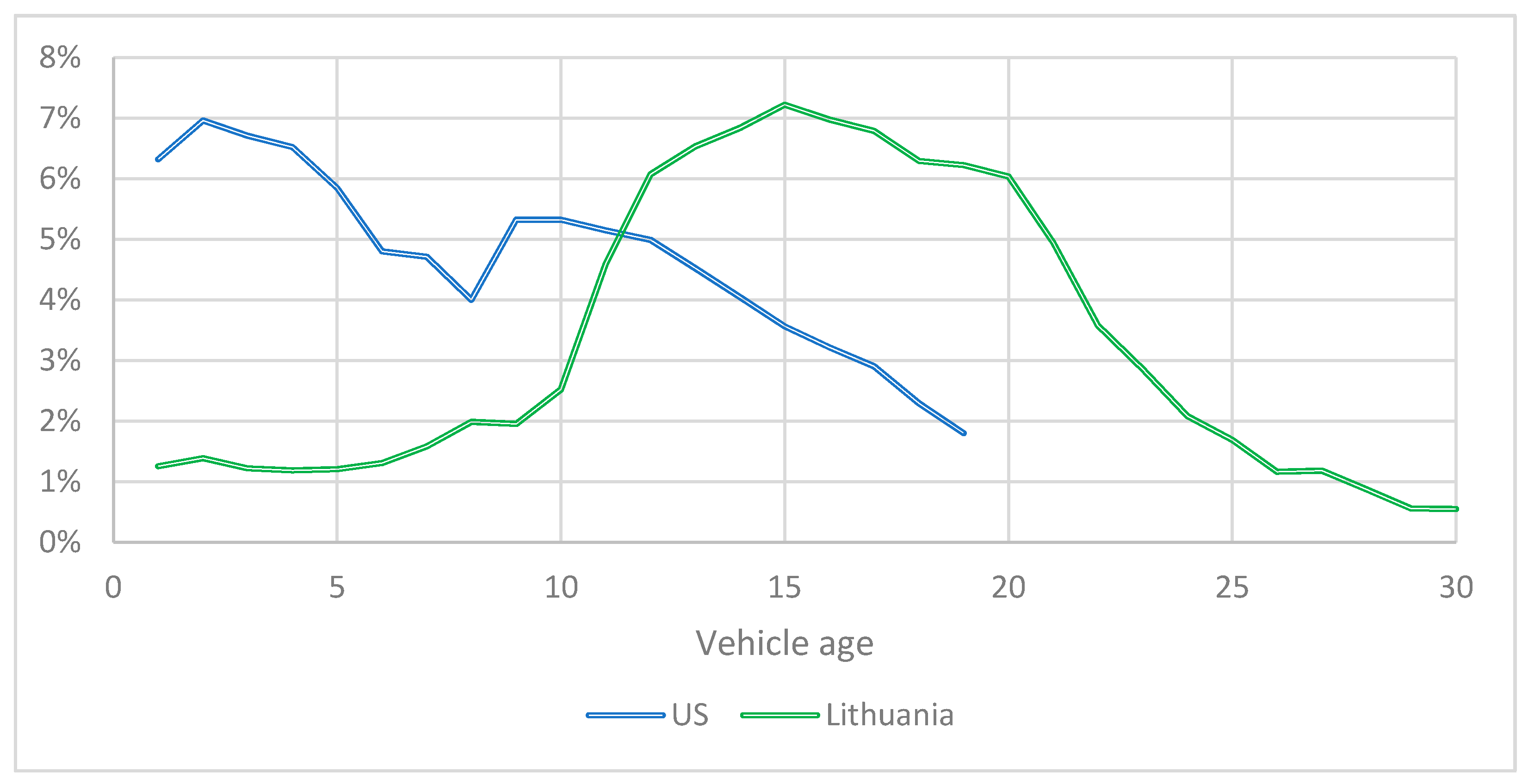
Differentiating vehicles by production year gives another benefit. It allows a better representation of the transport sector for smaller, less wealthy countries with access to the foreign second-hand car market. The wealthiest countries such as the United States have a declining vehicle age distribution curve (see Figure 1). Of course, there are some fluctuations due to economic reasons. This declining curve shows that vehicles taken out of stock are replaced by brand new ones. The vehicle age distribution curve for less wealthy countries, which have access to the foreign used car market, has an entirely different shape. It looks more like a bell curve (see Figure 1). In such countries, retired vehicles mostly are replaced by newer used cars from foreign countries. For example, in Lithuania, in 2018, only 1.2% of the car fleet was new cars. The biggest share was of 15-year-old cars with 7.2%. It is most likely that countries with such vehicle age distribution will lag in adopting new technologies in transport. For this reason, modeling vehicles by production year also improves the representation of fuel change.

2.1. Passenger Transport

In MESSAGE and many other energy planning models, demands are the model’s driving force because the model tries to satisfy set demands in a least-cost way. In the transport sector, there are demands for travel and delivery of goods. Travel demands can be expressed either in passenger-kilometers (pkm) or vehicle-kilometers (vkm). Different vehicle types have a different carrying capacity, i.e., 10 vkm traveled by bus satisfies the travel demand of more people than 10 vkm traveled by a personal car. Thus, it is more convenient to set demands for travel in pkm and delivery of goods in ton-kilometers (tkm).

These demands can be split further based on travel/delivery distance into several parts. For example, the TIMES-DK model has demands set for an extra short distance, short distance, medium distance and long distance [21]. In this paper, it will be split only into short (intracity) and long-distance (intercity) travel. This differentiation’s rationale is that certain travel/delivery modes are available only for specific travel distance. City buses can only be used for short-distance travel, while intercity buses are used for long. Furthermore, in long-distance travel, average travel speeds are higher, and internal combustions engines consume less fuel. As mentioned before, the energy planning model calculates the least-cost way to satisfy set demands. Therefore, the model has a constraint that travel supply has to be equal to the demands. In other words, the sum of passenger kilometers traveled by different travel modes must be equal to travel demands [19]:

$${{\displaystyle \sum }}_{y,f,a}PK{T}_{y,f,a,d}=PK{T}_d,$$

(1)

where $PK{T}_{y,f,a,d}$ is passenger transportation in pkm by vehicle type y (personal car, bus, train, etc.), fuel f (diesel, petrol, electricity, etc.), age group a (built before 1995, from 1995 to 1999, from 2000 to 2004, etc.) and travel distance d. Travel demand is denoted by $PK{T}_d$ (PKT stands for passenger kilometers traveled), where index d shows whether demand is for short or long-distance travel.

In the model, vehicles are represented by technologies, which have fuel and time from TTB as input. The use of travel time budget in energy planning models to enable modal shift was proposed by Hannah E. Daly [19]. This budget is based on Schafer’s findings [20], which show that on average people spend 1.1 h per day traveling, regardless of income, geographical or cultural settings. It includes travel by all modes, motorized and non-motorized. With higher income, people tend to travel longer distances, switching to faster transportation modes. In his paper, Schafer provides equations that help to estimate TTB for motorized travel based on traffic volume per capita [20]:

$$TT{B}_{mot}=a+\frac{b}{{\left(TV-c\right)}^d},$$

(2)

$$a=-\frac{b}{{\left(-c\right)}^d},$$

(3)

$$b=\frac{1.1}{\left(\frac{1}{{\left(240000-c\right)}^d}\right)-\left(\frac{1}{{\left(-c\right)}^d}\right)},$$

(4)

where c = −176,083 and d = 20. Schafer found that these values yield the best fit to statistical data.

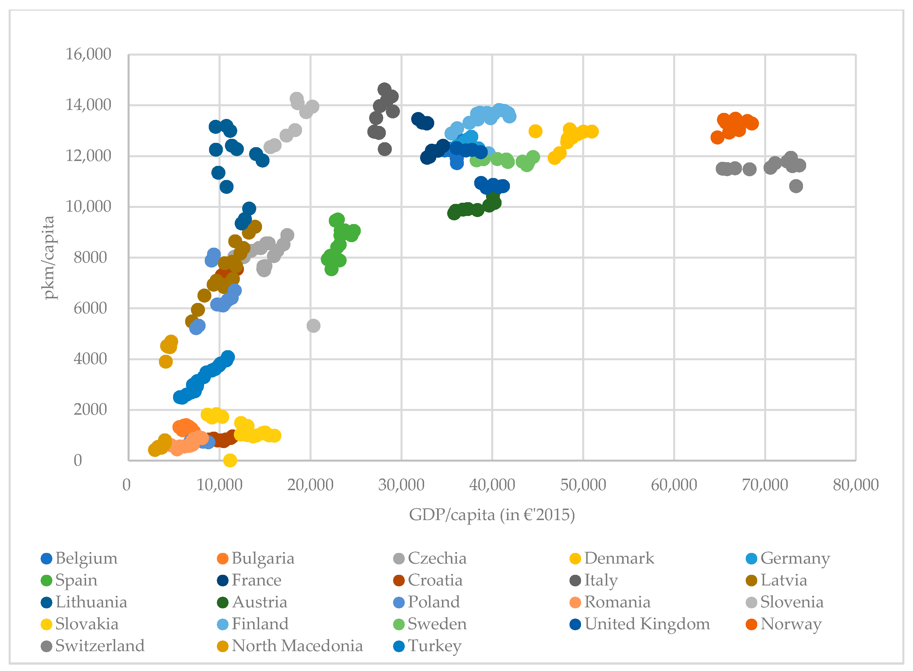
In our models, we used constant annual traffic volume per capita throughout the modeling years as Eurostat statistical data [34,35,36] show that traffic volume in road passenger vehicles per capita saturates at around 12,500 pkm/capita. See Figure 2.

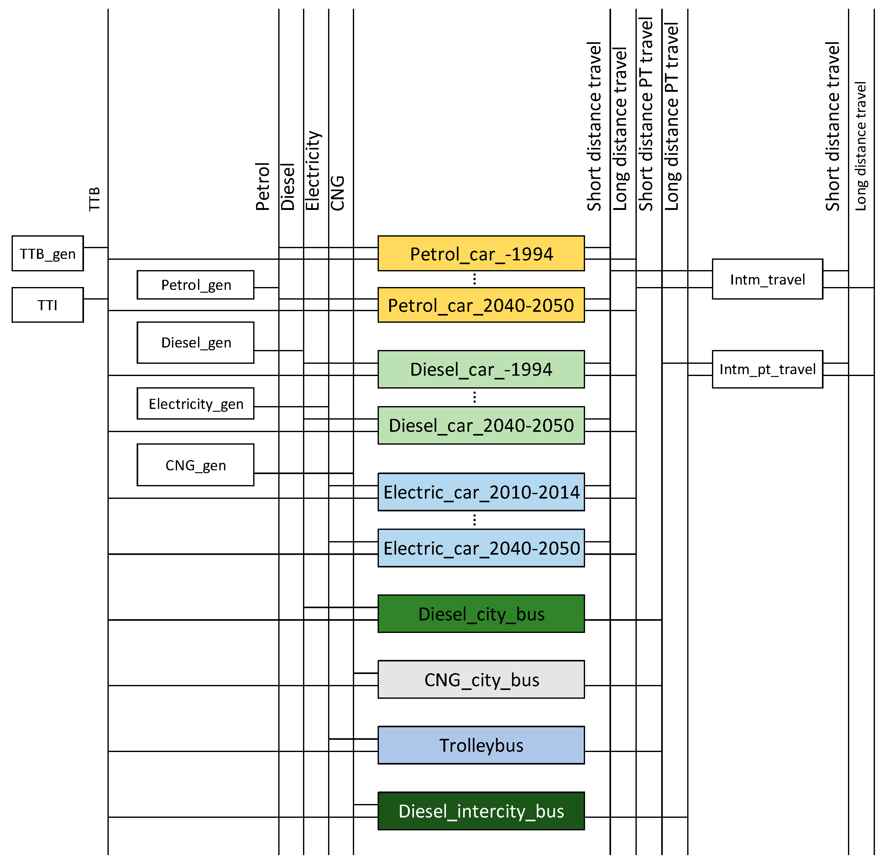
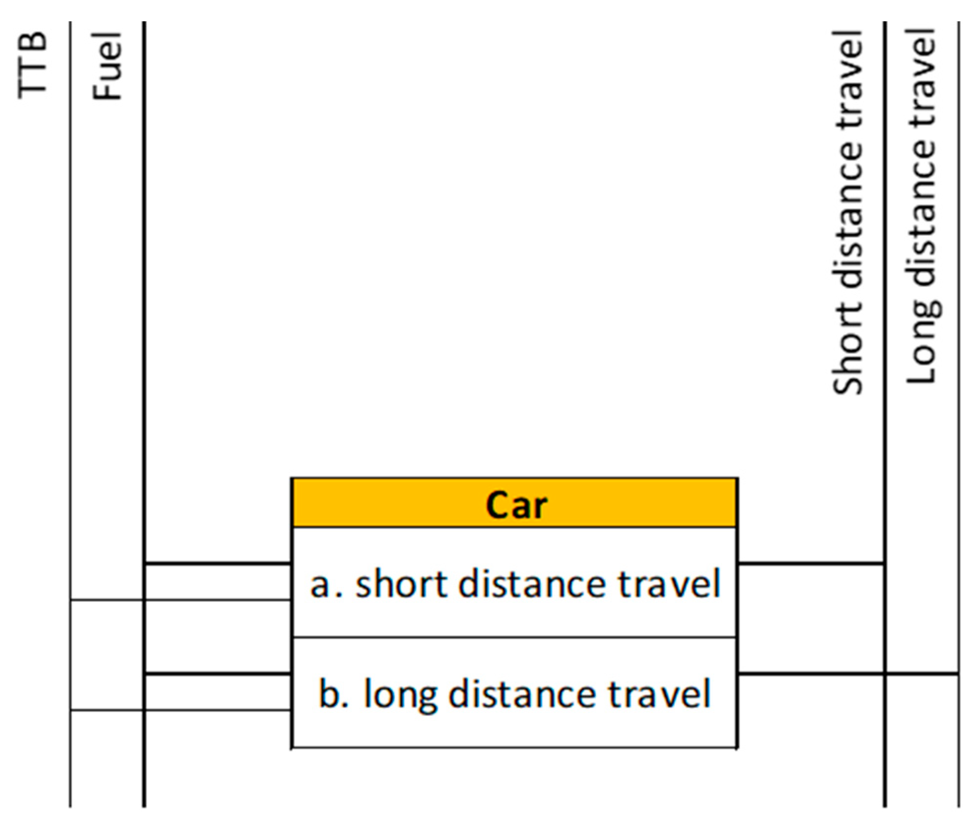
Modeled vehicle technologies output short or long-distance passenger transportation, or both, depending on vehicle type. For example, personal cars can be used for short and long-distance passenger transportation, so representing technology has two operating modes, one for short and one for long-distance travel. The principal diagram of modeling a car in the energy planning model is given in Figure 3. However, used quantities differ between the modes. Internal combustion engine (ICE) cars have a better fuel economy when driving between cities than when driving within a city because of less braking and accelerating cycles, less time stopped at traffic lights and higher efficiency at intercity travel speeds. Besides, due to higher speeds, it takes less time to drive the same distance.

Fuel economy $F{E}_{y,f,a,d}$ is calculated by dividing the vehicle occupancy rate $O{R}_y$ by its fuel consumption rate $FC{R}_{y,f,a,d}$ and multiplying it by 100. Here, the fuel economy is measured in Mpkm per 1 kt of fuel and fuel consumption rate in kg/100 km, while average vehicle occupancy rate is in persons.

$$F{E}_{y,f,a,d}=\frac{100·O{R}_y}{FC{R}_{y,f,a,d}}.$$

(5)

Time consumption rate is calculated with the given equation:

$$TC{R}_{y,f,a,d}=\frac{F{E}_{y,f,a,d}}{{\overline{v}}_{y,d}},$$

(6)

where $TC{R}_{y,f,a,d}$ is time consumption rate in million person-hours (Mph) per 1 kt of fuel. v_y,d is an average speed of vehicle type y in short or long-distance travel d in km/h.

At first glance, $TC{R}_{y,f,a,d}$ equation and measurement units might look very odd. However, in MESSAGE, secondary input has to be expressed in relation to the main one, in this case, to the fuel. Relations between inputs and outputs of vehicle technology can be described with two equations. The first one defines the relation between fuel consumption $F{C}_{y,f,a,d}$ (main input) and pkm produced (output):

$$F{C}_{y,f,a,d}=\frac{PK{T}_{y,f,a,d}}{F{E}_{y,f,a,d}}.$$

(7)

The second equation defines the relationship between secondary and main input, i.e., time consumption $T{C}_{y,f,a,d}$ and fuel consumption $F{C}_{y,f,a,d}$:

$$T{C}_{y,f,a,d}=F{C}_{y,f,a,d}·TC{R}_{y,f,a,d}.$$

(8)

Passenger transport capacity in the model is measured in Mpkm/year (how many million passenger kilometers can be traveled in a single year). So, the capacity of a single vehicle can be calculated by multiplying the number of hours in a year by the average vehicle occupancy rate $O{R}_y$ and average speed ${\overline{v}}_{y,d}$. Additionally, it should be multiplied by the operation time coefficient $O{T}_y$ because a vehicle is on the road only a part of the time. This coefficient prevents satisfying travel demands with too few vehicles.

$$C_{y,d}=\frac{365·24·O{R}_y·{\overline{v}}_{y,d}·O{T}_y}{{10}^6}.$$

(9)

Operation time for cars was estimated to be around 0.04, 0.55 for city buses and 0.2 for intercity buses.

Since vehicles travel at different speeds for short and long-distance travel, Equation (6) gives a different single vehicle capacity, depending on the speed used. For this reason, either short or long-distance travel mode has to be selected as a main activity in the model. In this paper, if a vehicle can be used for short and long-distance travel, short distance travel will be considered the main activity. Otherwise, the only option is the main one. In the model, the capacity for alternative activity is recalculated by multiplying the main activity’s capacity by the power relation coefficient.

$$C_{y,d=long}=C_{y,d=short}·P{R}_{y,d=long},$$

(10)

$$P{R}_{y,d=long}=\frac{{\overline{v}}_{y,d=long}}{{\overline{v}}_{y,d=short}},$$

(11)

where $P{R}_{y,d=long}$ is power relation (MESSAGE specific term) that defines the output ratio of alternative and main activities [14]. ${\overline{v}}_{y,d=long}$ is the average speed for long-distance travel and ${\overline{v}}_{y,d=short}$ is for short-distance travel.

2.2. Freight Transport

Freight transport can be modeled similarly to passenger transport, just with a few minor changes. $PK{T}_{y,f,a,d}$ should be substituted with $TK{T}_{y,f,a,d}$ (short for ton-kilometers traveled) and occupancy rate $O{R}_y$ with average cargo weight $AC{W}_y$. Units for $TK{T}_{y,f,a,d}$ are ton kilometers (tkm) and tons for $AC{W}_y$. Because of these changes, different units have to be used for $F{E}_{y,f,a,d}$, $TC{R}_{y,f,a,d}$ and $C_{y,d}$. Mtkm/kt is used instead of Mpkm/kt for $F{E}_{y,f,a,d}$, Mth (million-ton hours) is used instead of Mph for $TC{R}_{y,f,a,d}$ and Mtkm/year is used instead of Mpkm/year for $C_{y,d}$.

2.3. Vehicle Age Constraints

Vehicles in the model can be differentiated by their age group (e.g., built before 1995, from 1995 to 1999, from 2000 to 2004, etc.). Such differentiation gives the benefit of a better representation of fuel consumption and emissions from fuel combustion. Newer vehicles, on average, have better fuel efficiency due to ever-increasing environmental requirements.

Vehicle age distribution can be modeled by setting an additional constraint on produced travel by each vehicle age group. In this approach, each vehicle age group technologies are forced to produce a certain share of total Pkm. This share is derived from actual vehicle count by age. Separate constraints have to be set for each vehicle type for which vehicle age distribution is applied. For example, personal cars, built from 2005 to 2009, are constrained to produce 33.6% of Pkm supplied by all personal cars. It is recommended to create separate constraints for both short-distance and long-distance travel. Otherwise, the model might use newer cars for long-distance travel and older ones for short-distance travel or the other way around, depending on the assumptions. The general equation for such constraints is as follows:

$${{\displaystyle \sum }}_{f}PK{T}_{y,f,a,d}={\alpha }_{y,a,d}·{{\displaystyle \sum }}_{f,a}PK{T}_{y,f,a,d}.$$

(12)

The sum of Pkm produced by vehicle technologies of different fuels f but the same vehicle type y and same age group a have to be equal to the sum of Pkm produced by vehicle technologies of different fuels f and different age groups a, but of the same vehicle type y, multiplied by ${\alpha }_{y,a,d}$—the share of age group a in age distribution of the vehicle type y. Index d identifies if a constraint is specified for short-distance travel or long-distance travel.

The sum of shares of different age groups in vehicle age distribution for vehicle type y and travel distance d has to be equal to 1.

$${{\displaystyle \sum }}_a{\alpha }_{y,a,d}=1.$$

(13)

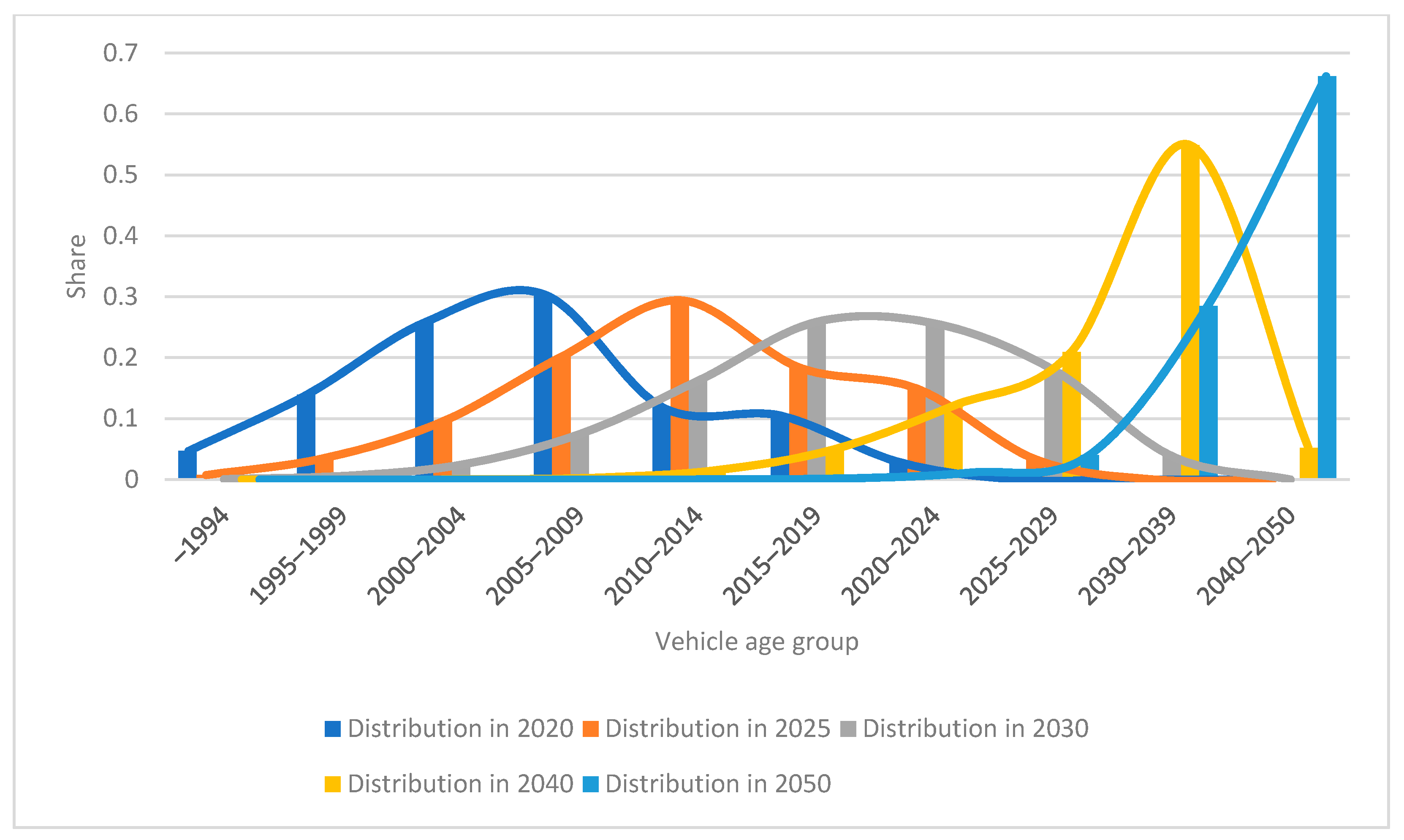
These shares must be recalculated for each modeling year so that vehicle age distribution remains constant or changes in an intended way. An example is given in Figure 4. In this figure, the vehicle age distribution of Lithuania was set to gradually change and reach a similar shape as in wealthier countries by 2050.

To apply these vehicle age constraints, separate equations have to be introduced in the model for each vehicle type, for which vehicle age distribution is to be applied, for each travel mode (short-distance or long-distance travel), vehicle age group and modeling year.

In Figure 4, the share of vehicles that were built from 2015 to 2019 increases in a period from 2020 to 2030. This means that used cars are bought in foreign markets. Used vehicles are cheaper, and generally, the older they are, the cheaper they are. To replicate this change in price within the transport model, investment costs should be decreased each modeling period after the period corresponding to the vehicle build year. It was estimated that passenger cars depreciate by 11.9% annually in Lithuania. The car depreciation rate was derived by evaluating how the average car price changed of 23 popular car models made in 2010 in ads placed on autoplius.lt website (most popular used car website in Lithuania) [37] from 2011 to 2019.

3. Results

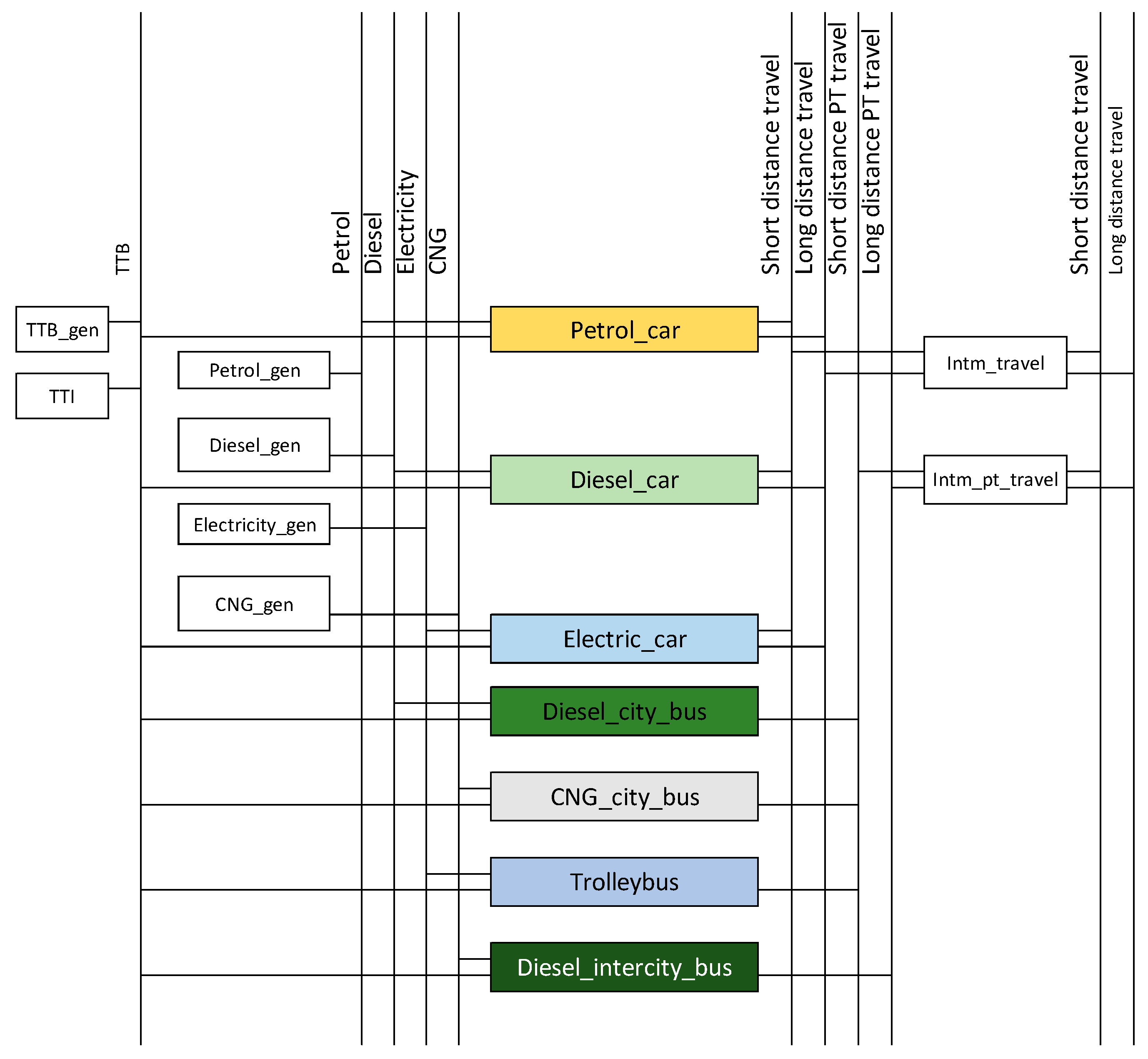
The proposed methodology was tested by creating two transport models using Lithuania’s transport data. In the first model, vehicles were modeled without considering vehicle age groups and vehicle age distribution, i.e., using the traditional approach (see Figure 5). In the second model, the proposed methodology was applied (see Figure 6). Models were run for the period of 2018–2050. Each year was modeled for 2018–2020, and 2020–2050 were modeled in 5-year periods. An 11% discount rate was used based on the discount rate for cars in Nikolas Hill et al. report for European Commission [38].

In Figure 5 and Figure 6, time for travel time budget (TTB) is produced by two technologies, TTB_gen and TTI. TTB_gen outputs time based on the assumption that, on average, people in Lithuania spend 0.829 h traveling on road transport per day. TTI can provide additional time for the budget but at a cost (0–5% TTB increase at 6 Eur/h, 5–10% at 12 Eur/h, 10–15% at 18 Eur/h, 15–20% at 24 Eur/h and >20% at 999 Eur/h). Petrol_gen, Diesel_gen, Electricity_gen and CNG_gen technologies produce fuels for the vehicles. Intm_travel and Intm_pt_travel are intermediate technologies used to separate demands and technologies that provide passenger transportation. This separation is required in MESSAGE for it to generate correct equations. Additionally, since these intermediate technologies sum the outputs of all car technologies (Intm_travel) and all public transport modes (Intm_pt_travel), it is convenient to use the output of these technologies instead of summing the outputs of separate vehicle technologies when defining vehicle age constraints.

Input data used to develop both models (Excel file S1: proposed approach.xlsm, Excel file S1: traditional approach.xlsm) as well as the model backup files (Model backup file S1: ProposedApproach.zip, Model backup file S1: TraditionalApproach.zip) are provided in the Supplementary Material.

It is important to mention that these models were designed for demonstrational purposes and do not represent Lithuania’s actual transportation system. A model with the proposed methodology applied is a simplified version of a far more detailed and complex model created within an ongoing DeCarb project. The newest version was deemed unnecessary and too complicated for the purpose of this paper.

In the results with the traditional transport modeling approach (see Figure 7), diesel cars remain the most used transportation mode only until 2020. From 2025, they are quickly overtaken by petrol cars as, within given assumptions, new petrol cars are more cost-efficient than new diesel cars. This is in part caused by a high discount rate of 11%. The higher the discount rate, the higher the weight purchase costs have when calculating discounted costs compared to the running costs. Diesel cars are cheaper to run, but petrol cars are cheaper to buy. In 2018, the share of petrol cars in total pkm traveled is 18%. By 2020, it increases to 23.6%, to 46.0% by 2025 and 69.1% by 2030. From 2030 to 2035, the share increases by an additional 7% and drops afterwards with increasing penetration of electric vehicles. Electric vehicles reach 11.5% of the total pkm traveled in 2040, 29.3% in 2045 and 62.9% in 2050. The share of travel using public transportation remains relatively similar throughout the whole modeling period, around 16–19%.

In short-distance travel, the most popular travel option is petrol cars. Even though fuel costs for petrol cars are higher than diesel and electric cars, lower investment costs make them a more economical choice for short-distance travel. However, the situation starts to change in 2040 when electric vehicle prices drop below petrol cars. After 2040, electric vehicles gradually replace petrol cars and in 2050 reach 86.8% of total pkm traveled in short distance travel. Diesel buses remain the most used form of public transportation until 2040. Afterwards, it tends to be gradually superseded by CNG buses.

Long-distance travel is provided mainly by diesel cars and diesel inter-city buses until 2025. From 2025, the use of petrol cars in long-distance travel increases rapidly and reaches 60% in 2030. Electric vehicles appear in long-distance travel only in 2050. However, the share rises sharply from 0% to 47.6%.

CO₂ emissions decline throughout the whole modeling period. The decrease between 2018 and 2035 can be explained mostly by decreasing travel demands (caused by a shrinking population) and ICE efficiency improvements from 2035 by increasing the share of electric vehicles.

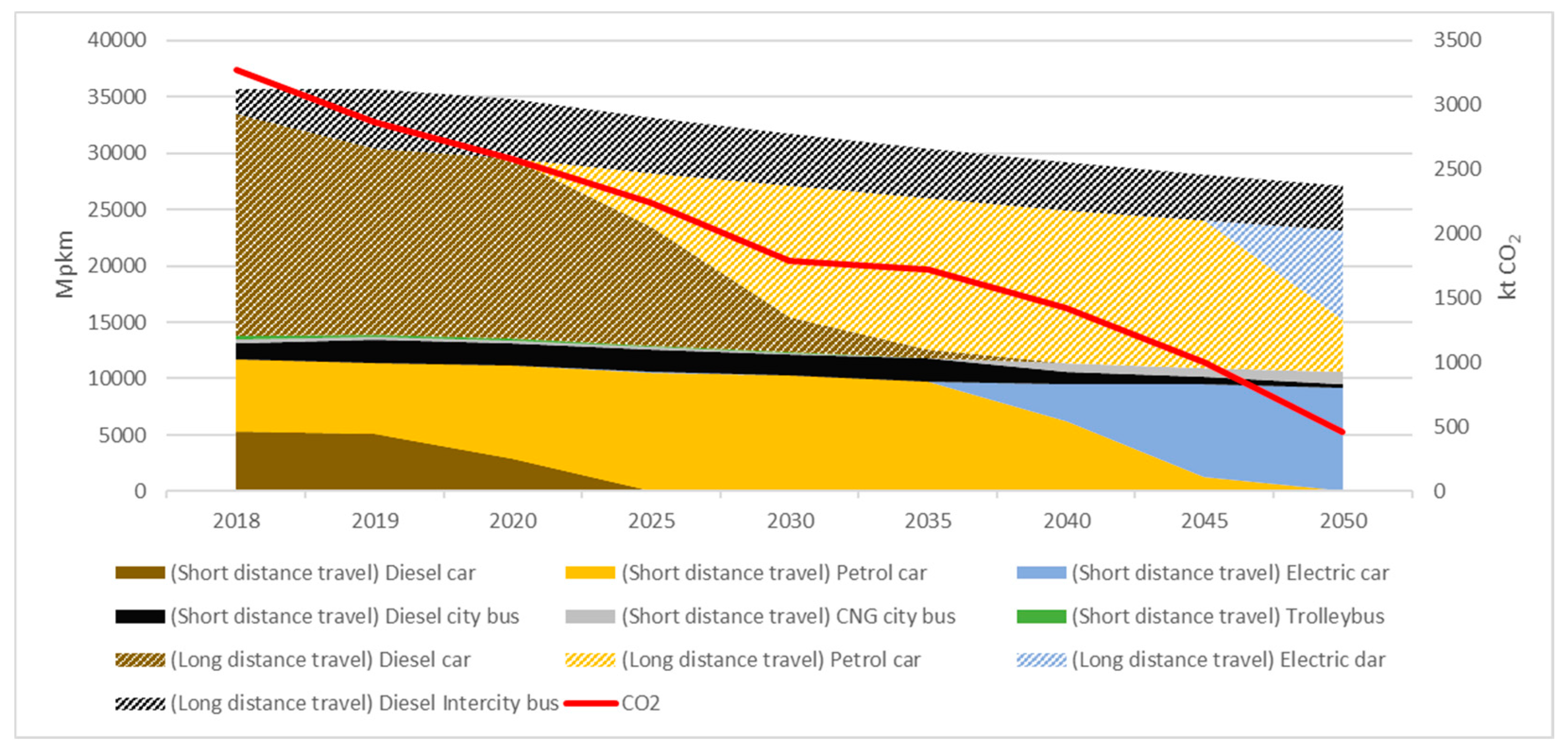
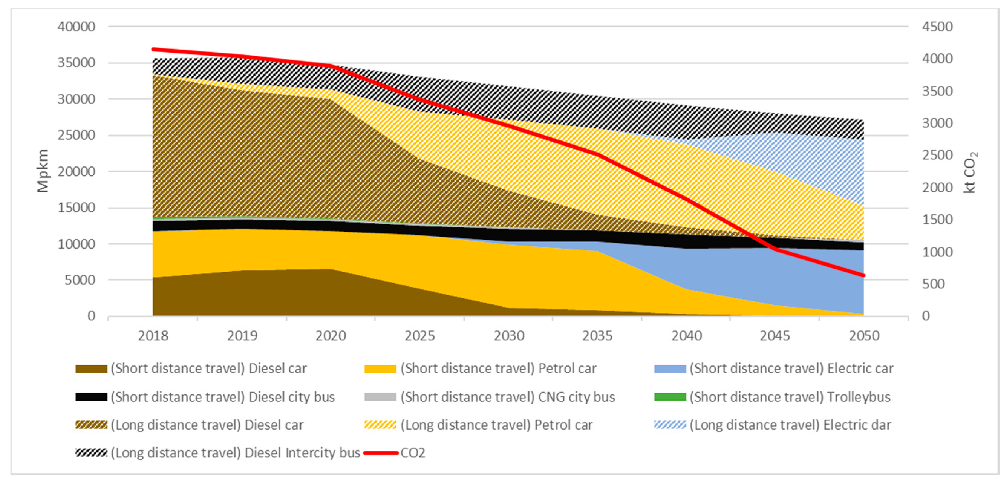
The results in the model with the proposed modeling approach are somewhat similar to previous ones. However, the transition to petrol cars and later to electric vehicles seems to be more gradual (see Figure 8). Petrol cars reach a share of 41.8% in 2025 instead of 46%. In 2030, it rises to 58.2% instead of 69.1%. The highest percentage that petrol vehicles get to is 66% in 2035. In the previous model, it was 75.9%. The use of electric vehicles starts to rise sooner. In 2030, it reaches 1.3% and in 2035 4.1%. By 2040, pkm traveled in electric vehicles jumps to 21.6%. In 2045, the share increases to 47.1%, and in 2050 to 66.5%. Diesel cars are completely phased out by 2050, a decade later than in the model with the traditional methodology applied.

In short-distance travel, the most popular transport mode is petrol cars, but just for the year 2018; later, for a short period from 2019 to 2020, they are superseded by diesel cars. This increase is seen in diesel cars made before 2009. After 2025, petrol cars once again have the highest share in short-distance travel and remain to do so until 2040. From 2030, the use of electric vehicles rapidly increases, and in 2040, the percentage of electric vehicles in short-distance travel rises to 49.5%, in 2045 to 72.5% and in 2050 to 83.3%.

In long-distance travel, petrol cars’ share increases from 2018, while in the model with a traditional transport modeling approach this only happens after 2025. The change using the proposed approach is more gradual. The share in 2020 is equal to 6.2% vs. 0%, in 2025 32.0% vs. 23.2%, in 2030 50.3% vs. 60.3%, in 2035 64.1% vs. 72.1% and in 2040 64.3% vs. 76.0%. In 2045, it is 51.9% vs. 76.0% and in 2050 28.2% vs. 28.4%.

The most apparent difference in the results of these two approaches is in CO₂ emissions. In the model with the traditional approach, they are significantly lower. In 2018, emissions are equal to 3275 kt CO₂ vs. 4150 kt CO₂. Our estimates for road passenger transportation emissions for 2018, based on the national GHG emission report [39], national statistics [40,41] and International Council on Clean Transportation [42] fuel consumption rates for heavy-duty vehicles are around 4480 kt of CO₂ (calculated by subtracting CO₂ emissions in road freight transport from emissions in whole road transport). Emissions using the traditional approach are 27% lower than estimated, while the proposed approach gives 7% lower emissions. This is a significant difference, considering that more than half of Lithuania’s CO₂ emissions come from the transport sector. The emission difference between modeling approaches is because, in the conventional method, cars of all ages are represented by a single technology. Only a single efficiency (that can change throughout the modeling years) can be entered for this technology. Usually, the efficiencies of new vehicles are used. It is possible to calibrate the efficiency to match the statistical data and externally calculate how the efficiency should change to match the shifting vehicle age distribution in modeling years. However, it requires an additional stock model and few iterations of calculations during the model runs. Our proposed approach endogenizes these calculations. We argue that our proposed approach has other benefits as well.

By comparing the results, we can see that transitions from one fuel to another are not that sudden when vehicle age distributions are applied, which is more realistic. Furthermore, in a model with vehicles represented by age groups, it is possible to model non-CO₂ emissions (CO, NOx, N₂O, NH₃, PM2.5) and emission taxes, which depend on production year/efficiency.

4. Discussion

The described transport modeling approach was developed within the integrated modeling and analysis of the deep decarbonization of the economy (DeCarb) project. The aim of this project is to develop a methodology and a system of models for the analysis of the least-cost deep decarbonization pathways of the economy. The modeling system consists of six linked models of energy, transport, industry, agriculture, household and other sectors.

We are aware that, for public transportation, a lower discount rate should be used. A societal discount rate could probably be used if state-owned companies run public transport. However, MESSAGE software allows entering a single discount rate. Therefore, sophisticated recalculations are necessary to be able to use two discount rates in the MESSAGE model. Such recalculations were performed when creating a transport model within the DeCarb project, but it was deemed unnecessary for this paper.

Further improvements made when creating a transport model for DeCarb include car representation by class (A-B, C-D, E-F, J-M), adding new car types (hybrid cars, FCEV), adding new public transportation options (electric buses and hydrogen buses for both short and long-distance travel, CNG buses and trains for long-distance travel), conventional fuel blending with biofuels, limits on how much new capacity can be added annually, vehicle registration taxes based on emissions and freight transport.

It was noticed that it is not easy to realistically represent behavioral choices in the transport sector using an optimization model. For example, the optimal solution might show that everyone should switch to electric vehicles by a certain year. However, the model does not consider that budgetary constraints refer to a significant part of the population. Additional improvements to the model are necessary to account for it. For this reason, it might be a good idea to model different population groups with different budgets for travel or at least a general budget constraint.

We also noticed that, to model the shift to electric vehicles adequately, travel demands should be split into more parts, not only in short and long-distance travel. Otherwise, the shift in long-distance travel might be too sudden. For this reason, we used an inconvenience cost for electric vehicles. Wróblewski et al. [43] provided data on travel distance distributions in urban and extra-urban modes, as well as insights on aperiodic failure costs that could prove very useful when developing a model with lower aggregation in travel distances.

Most of the methods that were applied to improve transport in energy planning models increased the size of the model. So, there is a risk that it will be too big to be hard linked to the power model, undermining the purpose of modeling transport in an energy planning model.

5. Conclusions

• We propose a new approach on how to improve transport sector modeling in energy planning models by differentiating vehicles not only by mode and fuel but also by age. It helps to improve the representation of fuel consumption and emissions in the model.
• In transport models, vehicle fleet age distribution constraints have to be set for smaller and less wealthy countries, which have access to large foreign markets of used cars, because a large share of vehicles taken out of stock is replaced by newer, used vehicles instead by new ones.
• The results of models with the traditional transport modeling approach and the proposed methodology applied were compared. The results show that the traditional modeling approach tends to have rapid changes in technologies, i.e., once one option becomes more economical, the model chooses to invest in it unrealistically too much. In the model with the proposed modeling approach, the technology shift is more gradual. Diesel cars are phased out by 2050, while in the model with a traditional approach, they are phased out by 2040. In the model with the proposed approach, the share of pkm traveled in electric vehicles begins to rise sooner from 2030, while in a model with the traditional approach it begins in 2040. In both models, electric vehicle penetration reaches a similar share by 2050 67% and 63%, respectively.
• Calculated 2018 road passenger transport CO₂ emissions with both approaches were compared to estimations based on statistical data. It was estimated that emissions in 2018 were around 4480 kt of CO₂. The output of the model with a traditional approach was 3275 kt of CO₂, while of a model with the proposed approach was 4150 kt of CO_2. This shows a significant improvement in the representation of CO₂ emissions and fuel consumption, as CO₂ emissions and fuel consumption are directly related.
• The proposed approach allows the modeling of emission taxes for vehicles depending on their age/efficiency.