Fault Detection in PV Tracking Systems Using an Image Processing Algorithm Based on PCA

Abstract

Photovoltaic power plants nowadays play an important role in the context of energy generation based on renewable sources. With the purpose of obtaining maximum efficiency, the PV modules of these power plants are installed in trackers. However, the mobile structure of the trackers is subject to faults, which can compromise the desired perpendicular position between the PV modules and the brightest point in the sky. So, the diagnosis of a fault in the trackers is fundamental to ensure the maximum energy production. Approaches based on sensors and statistical methods have been researched but they are expensive and time consuming. To overcome these problems, a new method is proposed for the fault diagnosis in the trackers of the PV systems based on a machine learning approach. In this type of approach the developed method can be classified into two major categories: supervised and unsupervised. In accordance with this, to implement the desired fault diagnosis, an unsupervised method based on a new image processing algorithm to determine the PV slopes is proposed. The fault detection is obtained comparing the slopes of several modules. This algorithm is based on a new image processing approach in which principal component analysis (PCA) is used. Instead of using the PCA to reduce the data dimension, as is usual, it is proposed to use it to determine the slope of an object. The use of the proposed approach presents several benefits, namely, avoiding the use of a wide range of data and specific sensors, fast detection and reliability even with incomplete images due to reflections and other problems. Based on this algorithm, a deviation index is also proposed that will be used to discriminate the panel(s) under fault. Several test cases are used to test and validate the proposed approach. From the obtained results, it is possible to verify that the PCA can successfully be adapted and used in image processing algorithms to determine the slope of the PV modules and so effectively detect a fault in the tracker, even when there are incomplete parts of an object in the image.

1. Introduction

PV generators are one of the most important renewable energy sources today. In fact, considering the power production, they are now the third most important behind hydro and wind energy generation [1]. PV generators can be used for small productions, such as domestic installations, or in high power plants. Their growing importance can be seen through the worldwide cumulative installed capacity, with a verified growth between 1995 and 2018, from 0.6 GW to 512 GW [2]. Most of the production is ensured by high power plants. Considering the 2018 value of the cumulative installed capacity, 180 GW were related to the utility-scale plants.

One of the problems associated with PV generators is the low efficiency [3], so it is extremely critical to ensure the maximum possible production. There are several factors that influence the production of the electrical energy from a PV panel, some being factors associated with the solar irradiation level, like the temperature of the PV panel, the wind velocity and the dust on the panels [4,5]; some of these factors are interrelated. For example, irradiance and dust have the same effect since if there is dust on the PV panel surface the irradiation is reduced. The same applies for wind and temperature, as when wind velocity increases, the temperature of the PV panel is reduced. However, to ensure the maximum solar irradiation, a fundamental aspect is related to the position between the PV modules and the brightest point in the sky. To ensure these conditions, several aspects should be considered, like the PV panels’ geographic location and the position of the sun [6]. In this way, the use of trackers associated with the PV panels play a very important role. Since this component has the ability to track the best position of the PV panels in relation to the sun, its use allows an important boost of the produced energy to be obtained [7]. Depending on the geographic location, the increase in the total yield that can be obtained by the sun tracking system can achieve values of up to 40% [8]. So, many solar power plants have adopted their use. There are two types of solar trackers: the single-axis and the dual-axis. The single-axis solar tracker panels rotate around a fixed axis [9]. In the case of the dual-axis trackers, the solar panels will move around two axes (Figure 1). Due to this, the solar panels can move in any direction and the best position of those panels in relation to the sun can always be achieved [10]. So, the increase in the yearly specific yield (generated power per unit of area) using solar tracking with the right tilt angle and direction are becoming more and more important. Some studies analyzed the positioning features of polycrystalline (p-Si), monocrystalline (m-Si) and amorphous silicon (a-Si) modules relative to the visible focus point of a reference concentrator photovoltaic module, under real meteorological conditions, using a dual tracking system [11,12]. These studies showed that the performance insensitivity thresholds of m-Si, p-Si and a-Si modules depended on the direction of the changes.

Solar trackers require the use of several components and systems, such as motors, motor drive, controllers and sensors [13]. Generally complex strategies of tracking with chips of microprocessors as control platforms are used [14]. Analyzing the operation and maintenance power plant reports it was assessed that the tracker systems were the major reason for the underperformance of the most significant PV power plant systems [15]. Therefore, a fault in one of these components will affect the correct position of the PV panels in relation to the sun, which will severely affect the optimum harness of energy that is possible to obtain from those panels. In this way, the existence of a fault detection system related to the PV panels’ tracker is fundamental to avoid important losses. A study about this problem in a real PV power plant (with an installed peak power of 2.15 MW) was able to verify that this problem is frequent [16]. In this case trackers with failed fuses were detected, and through the use of an algorithm proposed in that study, single fuse repair events were found quicker (5.31 days).

Due to the importance of PV systems in the context of renewable energy sources production, many works have addressed the fault diagnosis of such systems. However, most of them are focused on the parts of the PV systems that are not related to the trackers. On the other hand, most of the works are not related to the image processing. Nevertheless, the use of image processing has been an important tool in many systems. Examples of this are in agriculture [17], medical imaging [18], forensic dentistry involving the automatic identification of individuals based on their dental records [19], surface defect detection [20] or satellite imagery [21]. Image processing is also present in different areas of engineering, such as electrical engineering, with the detection faults found in electric motors [22], electrical capacitance tomography [23] or in the classification of solder joints in surface-mount devices [24]. It can also be found in chemical engineering, with fault detection and isolation of the Tennessee Eastman process [25] or in the ceramic and tile industry with surface defect detection [20]. Although in reduced numbers when compared with other approaches, image processing has also been used in solar energy. For example, it is widely used in thermal solar energy to calibrate the field of heliostat and to identify any fault in their orientation, compared to the optimum position [26,27]. Regarding the area of PV systems it is also used in several applications. One of the aspects in which this approach is used is for the detection of shadows in PV panels [28]. Another use is related to obtaining cloud cover indices. In this way, a method in which sky images and image processing are used to obtain forecasting models for direct normal irradiance is presented in [29]. Another interesting application is the one in which thermographic cameras are used for PV inspection [30,31]. One aspect related to these photovoltaic systems is that the PV panel is operated at its maximum power point (MPP). However, shadows could affect the algorithms for this operation. In [32] a global maximum power peak was proposed in which an optical camera to obtain the image of the PV panel was used to estimate the required irradiances. Another aspect related to these systems, especially related to the trackers, is the need for a sensor to direct the panels towards the sun. Thus, in [33], a position sensor based on camera and image processing was developed. Other studies explored the use of image processing for the detection of faults or degradations in PV systems. One of the parts of the system is related to the PV panel itself. In fact, with the passing of time the panels will degrade, also reducing their efficiency. Several methods appear to detect this degradation. In [34], a method in which the condition of the PV panels is verified through infrared images was presented. Another aspect related to faults of the PV panel, is the appearance of hot spots in their surface. Several works have proposed to detect those hot spots also through infrared images and image processing [35]. Regarding the detection of faults in PV panels’ trackers, in [36] a method based on image processing was proposed for the first time. The method is based on the concept that if one PV module is not aligned with the others, then there is a fault associated with the tracker of that PV module. With that approach, the inclination of the panels was determined using statistic moments and by the use of a line joining the centroids of two cells belonging to that PV module. However, that approach presents some limitations, since in some conditions it fails to detect the tracker under fault.

This paper is organized as follows: Section 2 focuses on the proposed machine learning method that allows detection of a fault in PV system trackers. This method uses a more simplified and non-conventional approach, namely, through the use of images and image processing algorithms, avoiding in this way the use of other types of sensors and a wide range of data. The image processing algorithms determine the points of all the cells of the PV modules and the assignment of each point to the correspondent module are described. The use of the PCA algorithm that uses the coordinates of the points of each module to determine their orientation is also innovative and presented in this section. First, the points of the PV cells detected by the image processing algorithms are clustered in each of the existing PV modules in the image. Then, the position (coordinates) of those points is used in the PCA based algorithm to determine the orientation of the PV module. In Section 3, several tests are presented and discussed with the objective to analyze the efficiency of the proposed method and the fast and reliable determination of the inclination. Finally, conclusions are drawn in Section 4.

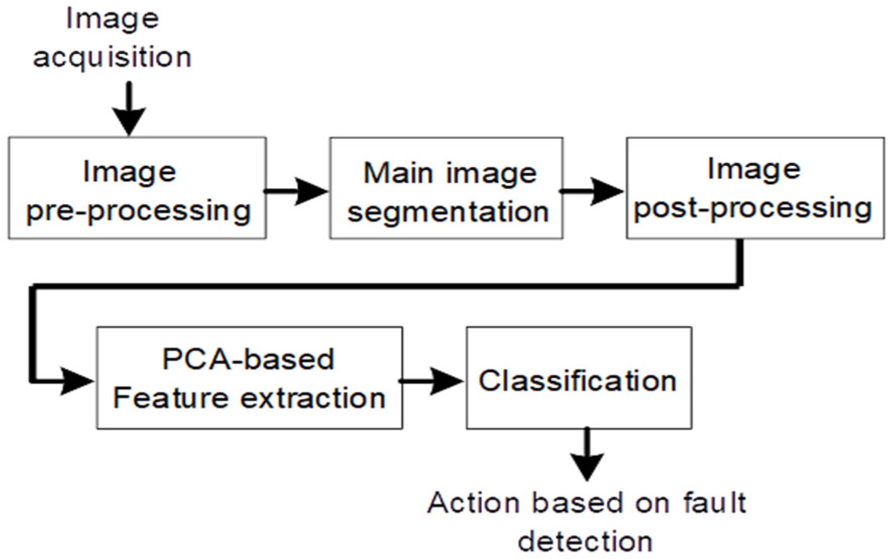
2. Proposed Image Processing Algorithm for Fault Detection of Tracking Systems

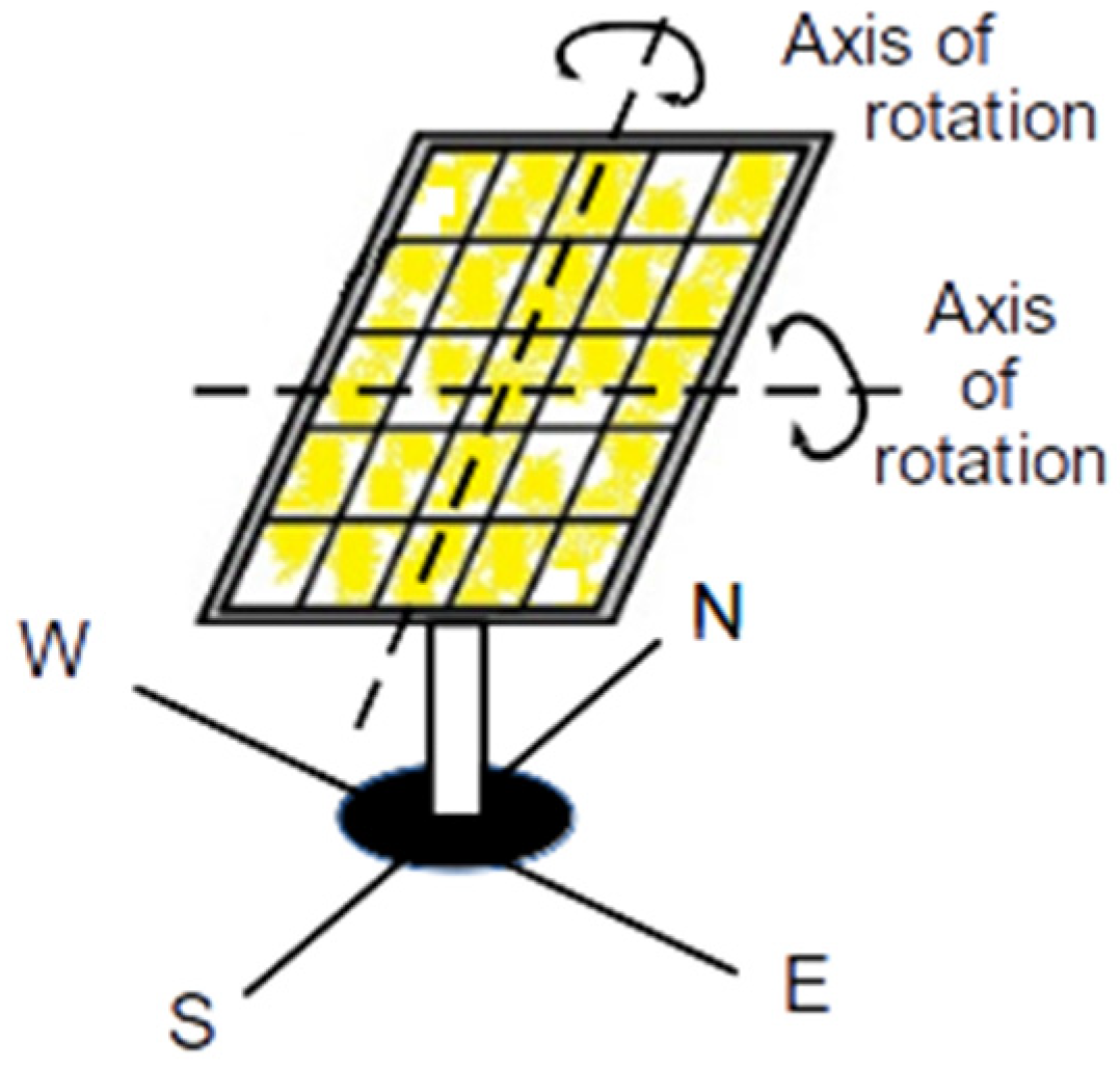
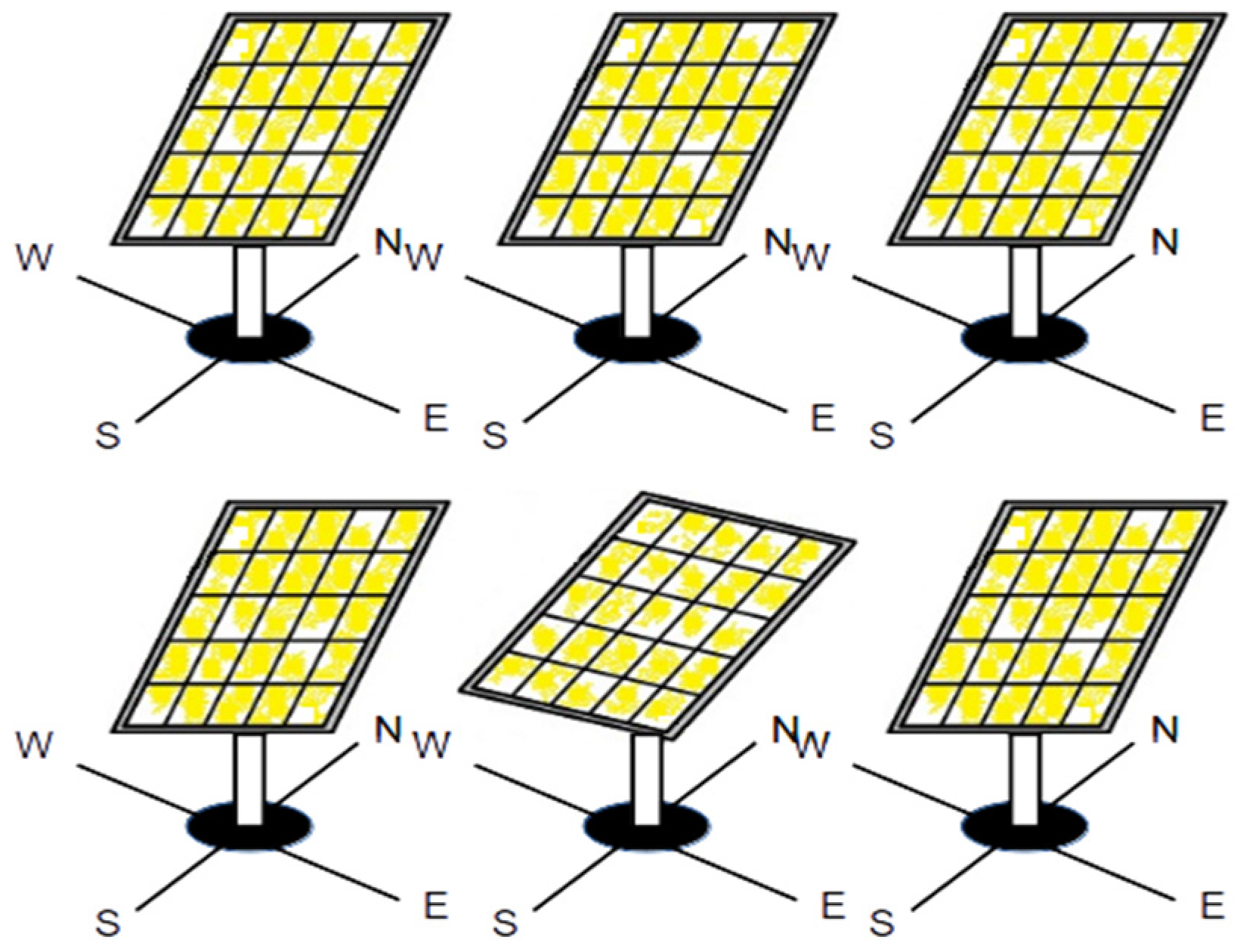
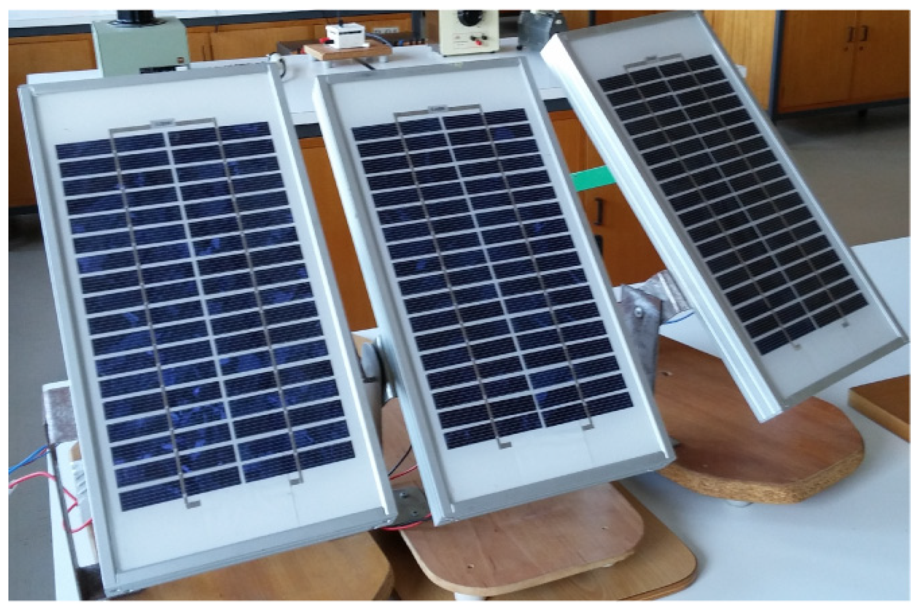
2.1. Proposed Strategy

Although the use of trackers allows the optimization of PV systems regarding the maximum energy production by the PV panels, they will introduce more complexity to the system by which they will be subject to new failures. In fact, these trackers consist of several components and systems that are prone to failure, such as motors, motor drive, controllers and sensors [13]. In this way, a failure in one of these components will greatly affect the energy generated by the PV panels since it will not ensure that their orientation will be at the brightest point in the sky. Due to the cost of the trackers, usually they are used in large systems, like PV and thermal solar power plants. So, due to the high number of these systems, usually the identification of a fault in a tracker can be complex and long. According to previous studies [16,37,38], operators often just visualize the daily gain of the plant, in order to obtain an impression of the amount of energy produced. Even dedicated software systems for monitoring renewable power plants are often limited to features like storing and visualizing measurement data [39]. Analysis algorithms used in practice, often are just simple threshold calculations. In this way, malfunctions that appear in the PV power plant that do not lead to an immediate total power loss, may go unnoticed for a long time. To speed up this process, a SCADA system and many sensors to monitor numerous parameters can be installed in PV plants. Thus, the use of images to detect this kind of fault becomes much more simple and easy to implement. On the other hand, due to the existence of several PV systems, a pattern recognition method can be implemented through the comparison between them. So, considering that the number of PV systems with a fault in a tracker is in a much lower number of PV systems (usually a single one), the detection of a fault can be implemented through the comparison of the slopes between them (Figure 2). In reality the orientation of the PV systems with no fault in the tracker will be exactly the same since they are oriented to the sun. However, the one with a fault in that system will present a different orientation. In this way, analyzing the orientation of the PV panels’ slope, if there is one or more (but the minority) with a different orientation of the healthy, then that (or those) PV system(s) has a fault in the tracker.

The identification of a PV system tracker fault through the detection of the PV panel’s slope can be realized by a simple photograph instead of the use of complex methods. So, in association, a pattern recognition method must be used. In this case, an approach for the feature extraction that uses the principal component analysis (PCA) is proposed, stressing that the PCA has been used in many industrial applications [40,41,42,43]. However, it has not yet been used in image processing to detect slopes of certain objects, as is the case of this problem. So, for the implementation of this approach five main steps were considered, more specifically: image pre-processing, main image segmentation, image post-processing, PCA based feature extraction and feature based classification. The steps of the proposed approach can also be seen in Figure 3.

The first step is associated with the image processing, namely to identify and isolate the PV panels that are inside the photograph. For this image treatment, the histogram analysis technique was adopted, through which the feature extraction of the several regions that exist in the image will be obtained. In this way, the regions associated with the PV panels will be isolated. Since the purpose of the approach is only to identify the PV panels, the pixels that are not associated with those panels will be converted to white, allowing simplification of the analysis. On the other hand, the RGB image will be converted into a binary image through the Otsu method, which defines an automatic threshold value [44]. The morphological operators to separate the several regions were also used, with the purpose of isolating the region associated with the PV panel. The image segmentation is the second step of this approach. For this segmentation, the Blob coloring algorithm will be used [45]. The result of this algorithm gives a divided binary image (regions), in which the black pixels are associated with the regions, while the white pixels are associated with the background. Usually there are regions that do not belong to the PV panels, being removed in the next step (third), image post-processing. In this third step only the regions that are associated with the cells of the PV panels will be selected. The identification of these regions will be realized through a set of features, namely, region solidity and area, index of compactness and eccentricity. One problem that could appear in the image post-processing is related to the fact that some PV cells might not be detected by the camera due to the existence of an obstacle or very low image quality. In this case, those cells will be eliminated, although incorrectly, which means they will not be used for the determination of the PV panel orientation. In this way, the proposed algorithm was developed to determine the PV panels’ orientation even with a small number of cells. As said, the orientation of the PV panel will be realized through the identification of their cells. In this way, to identify the cells associated with each PV panel the single-link clustering algorithm was used [46]. Thus, since the orientation of each PV module is based on their PV cells then it is necessary to know what PV cells are assigned to each PV module. The single-link clustering method has been used in cluster analysis but since it was applied in different application areas and with many different computational algorithms it is also known by other names such as the nearest neighbor method or the connectedness method.

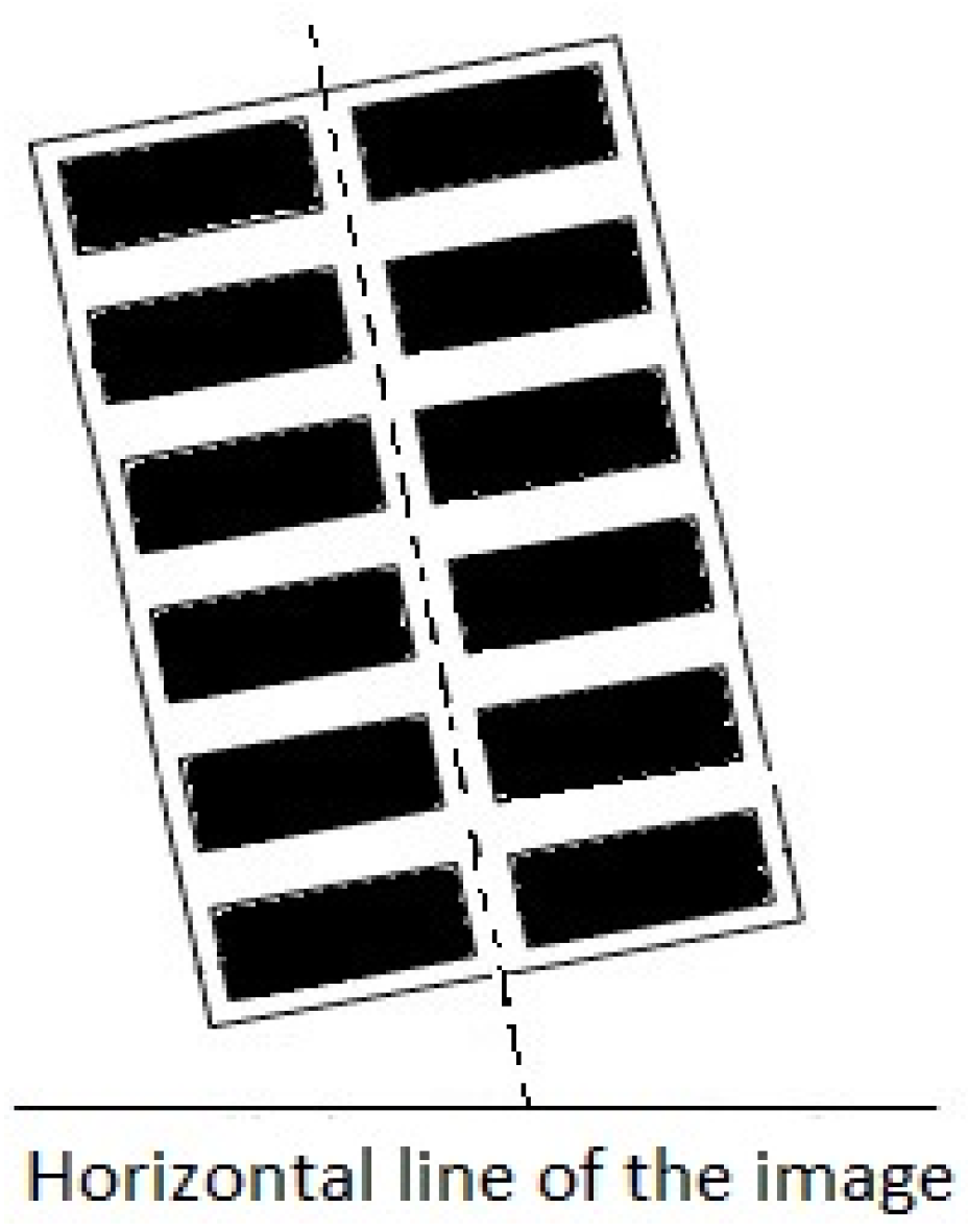
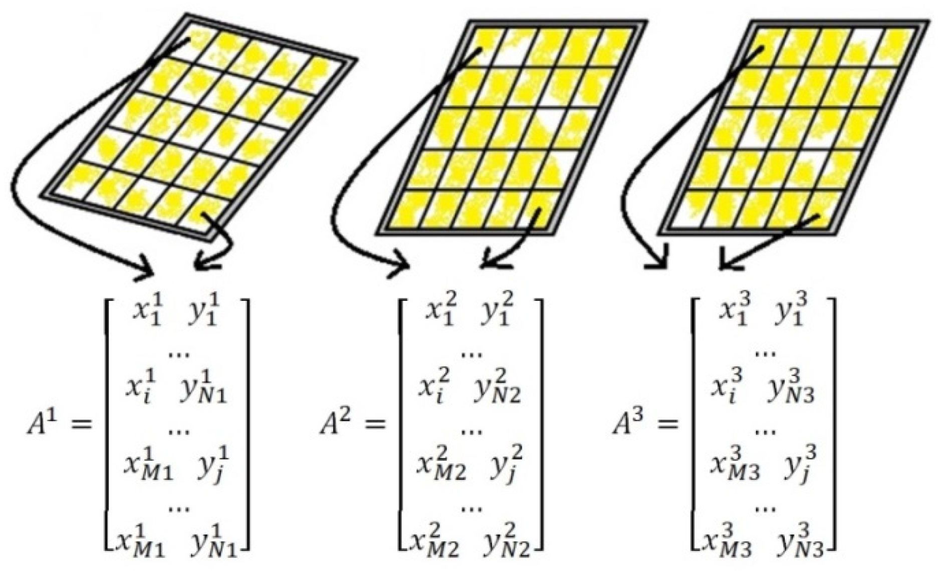
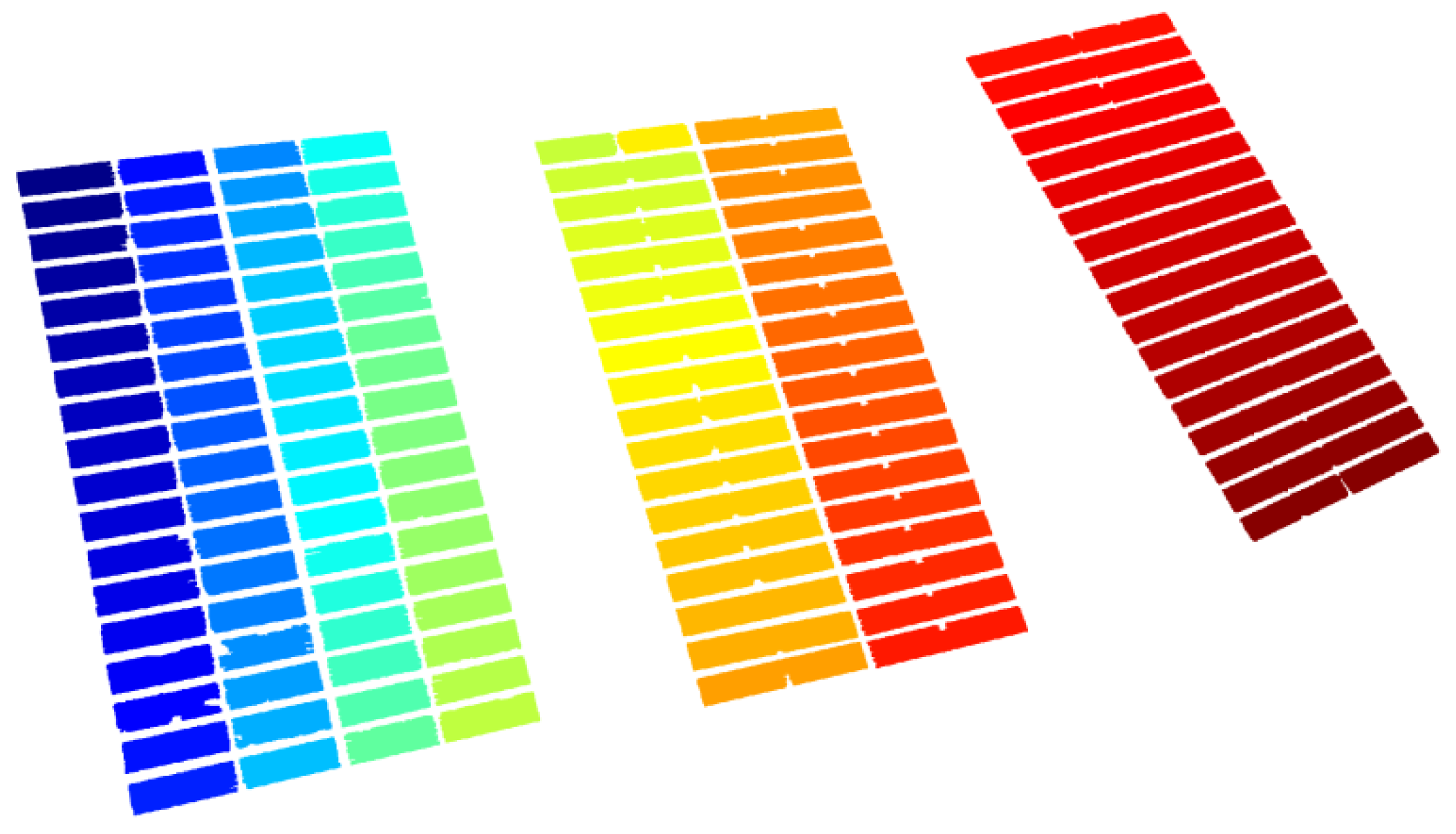
2.2. Image Processing Approach Using PCA

In the proposed approach the objective of the clustering is to group the pixels of the image that belong to the PV cells into a system of sets (PV modules having the single-link criterion the minimum Euclidean distance). In the beginning, each pixel belonging to a PV cell is a small cluster that represents a PV module resulting in a weakest clustering. The small clusters, separated by a threshold distance level, Th_L, between them, are then combined to form larger clusters (strongest clustering) until the number of clusters (PV modules) reaches the number of PV modules in the image. Thus, at a given threshold distance level, Th_L, the clusters consist of the sets of pixels for which such chains exists for all pairs of pixels within the same cluster. Since each pixel belongs to only one cluster (PV module) therefore the clusters will be non-overlapping at a given threshold distance level Th_L. Considering the clusters C₁ and C₂, the linkage function using the smallest distance between pixels in the two clusters is given by [47]:

$$D\left({\mathrm{C}}_1,{\mathrm{C}}_2\right)=\min \left(dist\left({\mathrm{p}}_{1\mathrm{i}},\hspace{1em}{\mathrm{p}}_{2\mathrm{j}}\right)\right),\mathrm{i}\in \left(1,\dots ,n{c}_1\right)and\mathrm{j}\in \left(1,\dots ,n{c}_2\right)$$

(1)

and

$$dist\left({\mathrm{p}}_{1\mathrm{i}},{\mathrm{p}}_{2\mathrm{j}}\right)=\sqrt{{\left({\mathrm{x}}_{1\mathrm{i}}-{\mathrm{x}}_{2\mathrm{j}}\right)}^2+{\left({\mathrm{y}}_{1\mathrm{i}}-{\mathrm{y}}_{2\mathrm{j}}\right)}^2}$$

(2)

being $dist\left({\mathrm{p}}_{1\mathrm{i}},{\mathrm{p}}_{2\mathrm{j}}\right)$ the distance of the Euclidean between the pixels of clusters C₁ and C₂. The (x_1i, y_1i) and (x_2j, y_2j) are the coordinates of ith pixel ${\mathrm{p}}_{1\mathrm{i}}$ and jth pixel ${\mathrm{p}}_{2\mathrm{j}}$ that belong to the clusters C₁ and C₂. The parameters $\mathrm{n}{c}_1$ and $\mathrm{n}{c}_2$ represent the number of pixels in the clusters C₁ and C₂, respectively. If the smallest distance between the clusters C₁ and C₂ is less than a given threshold distance level Th_L then they are united into a single cluster.

To determine the orientation of the PV modules it is proposed to use PCA theory. This is a widely used statistical procedure that has been used in many applications [48,49]. However, this theory has not yet been used to determinate object slopes in image processing. In accordance with this theory, the first principal component is the one where the data have more energy when compared with the remaining directions. In this approach, the principal component, containing the most data energy of the points belonging to each of the PV modules, gives their orientation. In Figure 4, points of the cells used in the PCA algorithm can be seen and the orientation of the principal component that corresponds to the orientation of the PV module. After the clustering stage, each point, corresponding to the PV cells, are assigned to a specific PV module. The cartesian coordinates of those points constitute the data sample matrix used in the PCA algorithm. In Figure 5, an example of three matrixes for three PV modules can be seen where the points used are represented by the yellow color.

The number of significant samples, Mi, corresponds to the number of rows of the matrix Ai. The number of rows of the matrixes A1, A2 and A3 is different and depends on the number of points of each PV module, obtained after the threshold and clustering procedures. The first column of each matrix has the x coordinate of each point and the second column has the correspondent y coordinate of that point. Before applying the PCA algorithm, it is necessary to subtract the mean from each of the two data dimensions x and y. The mean subtracted, $A_{AV}^i$, is the average across each dimension (3). So, all the x coordinate values have a mean value subtracted, and all the y coordinate values have a mean value subtracted from them. This produces a new data set, $A_{flt}^i$, whose mean is zero (4).

$$A_{AV}^i=\frac{1}{Mi}{{\displaystyle \sum }}_{j=1}^{Mi}{A}^i$$

(3)

$$A_{flt}^i=A^i-A_{AV}^i$$

(4)

From the new data set, the symmetric covariance matrix between the x and y dimensions is computed (5).

$$Co{v}^i=\frac{1}{Mi}\ast A_{flt}^i\ast {\left(A_{flt}^i\right)}^T$$

(5)

After establishing the correlation matrix of $A_{flt}^i$, its eigenvectors, $U^i$, and the correspondent eigenvalues, $E^i$, are determined by (6) [50,51].

$$Co{v}^i{U}^i=U^i{E}^i$$

(6)

where

$$E^i=\left[\begin{array}{c}val{p}_1 0\\ 0 val{p}_2\end{array}\right]$$

(7)

$$U^i=\left[\begin{array}{c}vect{p}_{x1} vect{p}_{x2}\\ vect{p}_{y1} vect{p}_{y2}\end{array}\right]$$

(8)

The determination of the PCA is usually used to reduce the data dimension. However, instead of that, it is proposed to use this theory to determine a slope of an object through image processing. Thus, in order to use this theory to determine a slope, it will be considered the eigenvector $\left({vectp}_x,{vectp}_y\right)$ associated with the highest eigenvalue $\left(valp{\_}_{max}\right)$, and the orientation of the ith PV module will be obtained by (9).

$${\theta }^i=ta{n}^{-1}\left(\frac{{vectp}_y}{{vectp}_x}\right)$$

(9)

It should be understood that the eigenvector associated with the highest eigenvalue represents the principal component. The sign of the eigenvalue is not important because the orientation of the PV module is given only by the principal component direction. Since the eigenvalues are real values, the correspondent eigenvectors are orthogonally. The angle computed by (9) will allow for the determination of the orientation of each PV module. In this way, through the feature associated with the orientation of each PV panel it will be possible to detect a fault in the PV trackers. Due to the existence of small inaccuracies associated with the trackers, as well as small errors that can appear in the determination of the slope angles, the comparison of each PV panel orientation with the others will be realized through the average value of the panels’ slopes with a higher occurrence. To realize this, the average value of the orientation will be given by (10). Parameter T represents the number of panels where their angles belong to the set of angles of higher occurrence and ${\theta }^i$ are their corresponding angle values.

$${\theta }_{AV}=\frac{1}{T}{\displaystyle \sum }_{i=1}^T{\theta }^i$$

(10)

To detect a fault in the tracker of each PV panel, the difference between the average value of the slopes and the slope angle of each panel should be higher than a predefined threshold level. In order to ensure sensibility and reliability in the detection of failures, the system must be initially calibrated by acquiring several images throughout the day and analyzing the maximum discrepancy obtained between healthy trackers. Based on this analysis, the threshold level is then defined. After this calibration, the threshold value can be defined, which should be higher than the maximum deviation from the average value of the angles of higher occurrence. Considering that the maximum deviation that is possible between PV panels is 180°, then the following deviation index (DI) is defined by:

$$DI=\frac{\left|{\theta }^i-{\theta }_{AV}\right|}{180}\times 10$$

(11)

where θⁱ is the slope of the PV panel and θ_AV is the average value of the PV panels’ slopes.

To state that in a real system the angles of panels of the healthy trackers practically will present the same value, by which the resolution can be lower than 1 degree, or lower than 0.01 deviation index (DI). However, since this precision is not needed, one recording every 15 min is more than enough, and higher angles (or deviation indexes) are recommended. However, it is recommended to acquire several images throughout the day and to analyze the maximum discrepancy obtained between healthy trackers and use that value as the minimum threshold value.

Based on the DI parameter, the algorithm used in the identification of the faulty PV tracker is described in the following steps:

• Step 1: Determine the average value of the orientation using (10);
• Step 2: For each panel under analysis determine the corresponding orientation and deviation index using (9) and (11), respectively;
• Step 3: Compare the deviation index (DI) of each panel with the predefined threshold value, Th:
• Step 3 (a)—If DI_i ≤ Th, then the ith panel are in healthy condition;
• Step 3 (b)—If DI_i > Th, then the ith panel is considered with a fault in their tracker—the ith panel is removed from analysis and return to Step 1.

One disadvantage of this approach is inherent to vision-based systems, which is the image quantization. Increasing the distance between the camera and the panels causes the decrease in the resolution of the regions in the image containing the panels. Another disadvantage arises in the situation in which the PV cells are not in the camera field of vision, as for example, due to obstacles, making this region of the panel not to be used in the correct determination of its slope angle. When this situation occurs, the region that is covered up is removed in a previous step (post-processing step).

3. Results

The capability of the proposed approach to identify faults in PV trackers was tested using several images with PV panels. Those images include panels in which some of them present the same orientation and others with a different orientation indicating a fault. In accordance with this, several tests were realized, considering situations in which there is not any fault, others with fault but with different conditions, such as, different slopes for the healthy and faulty panels. The implementation of the proposed method was realized using the program Matlab.

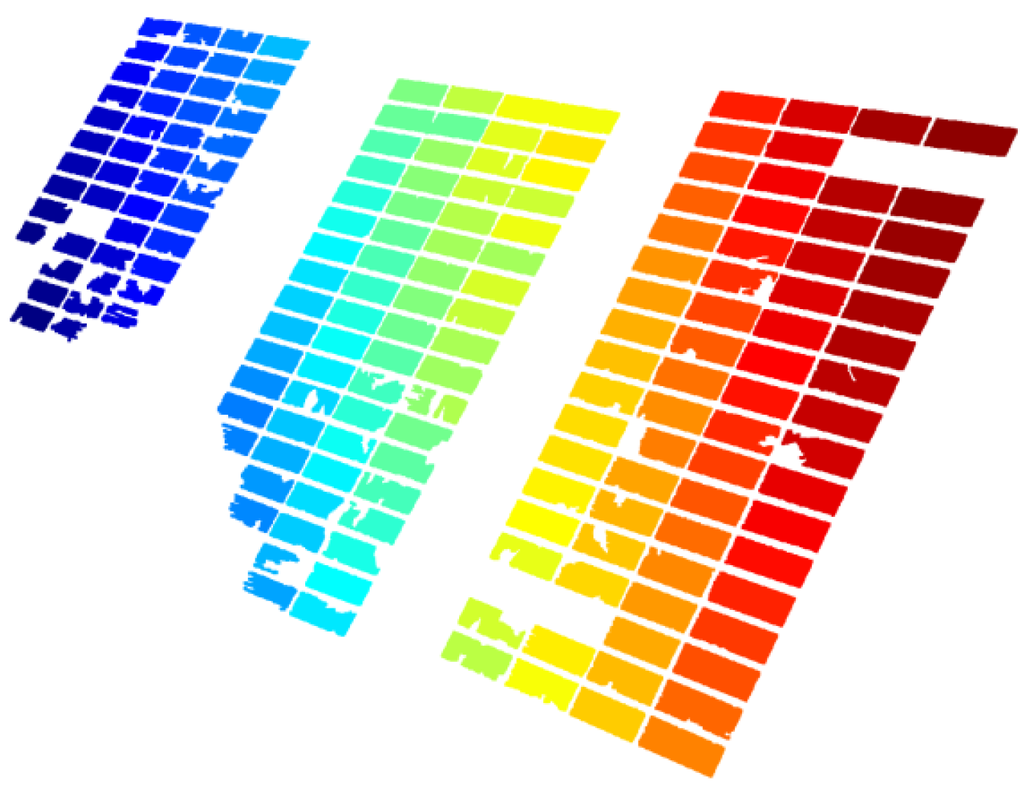
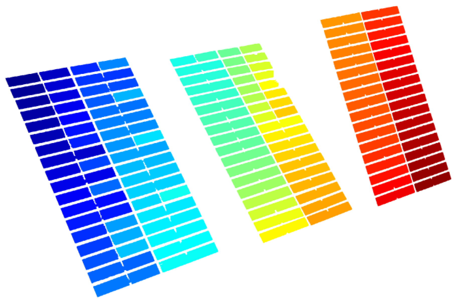
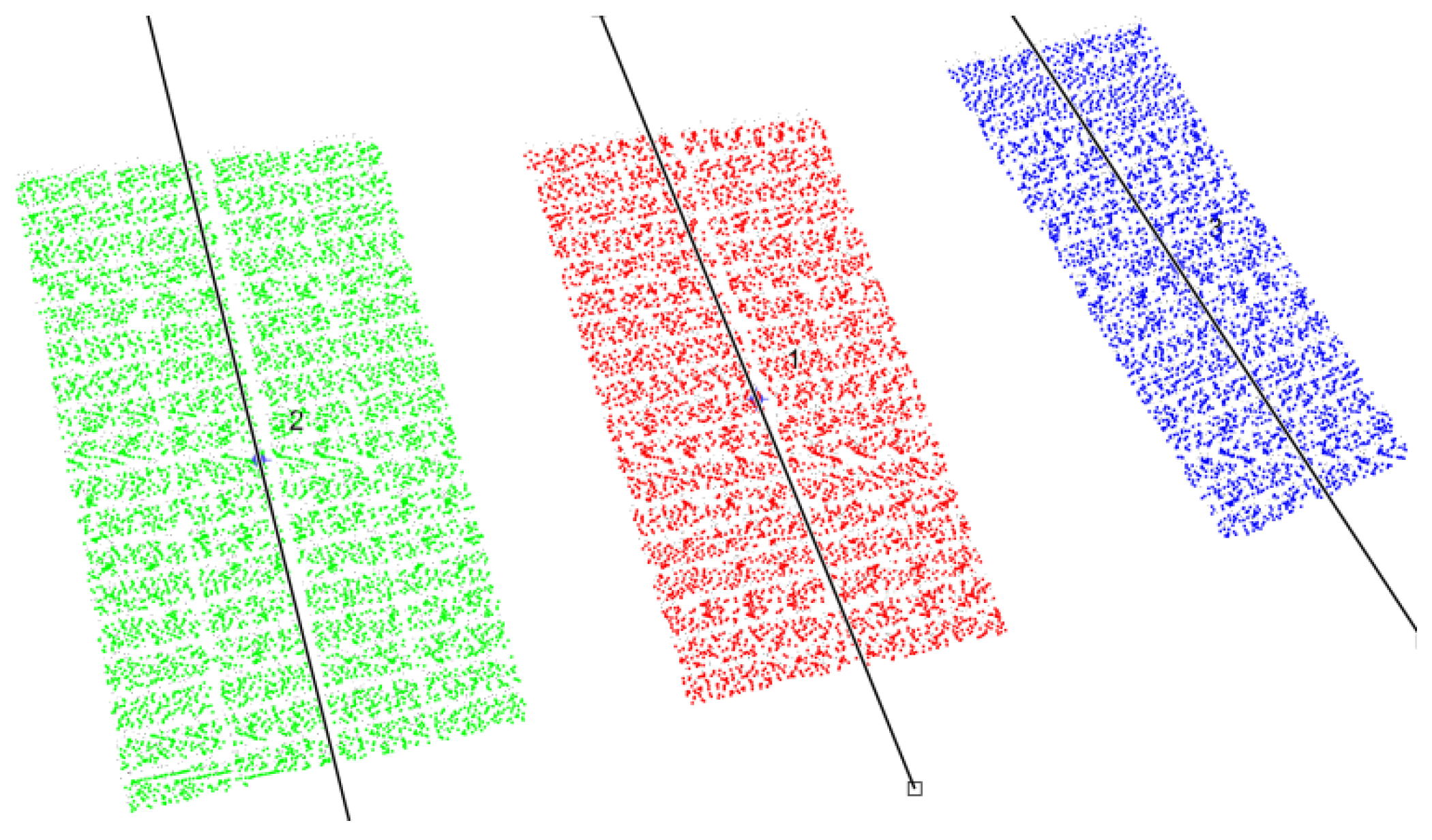
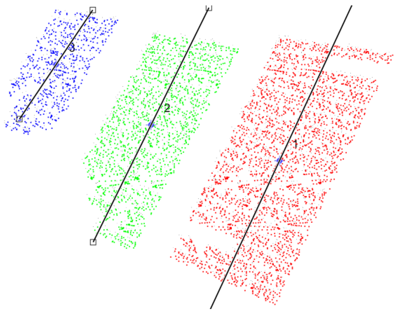
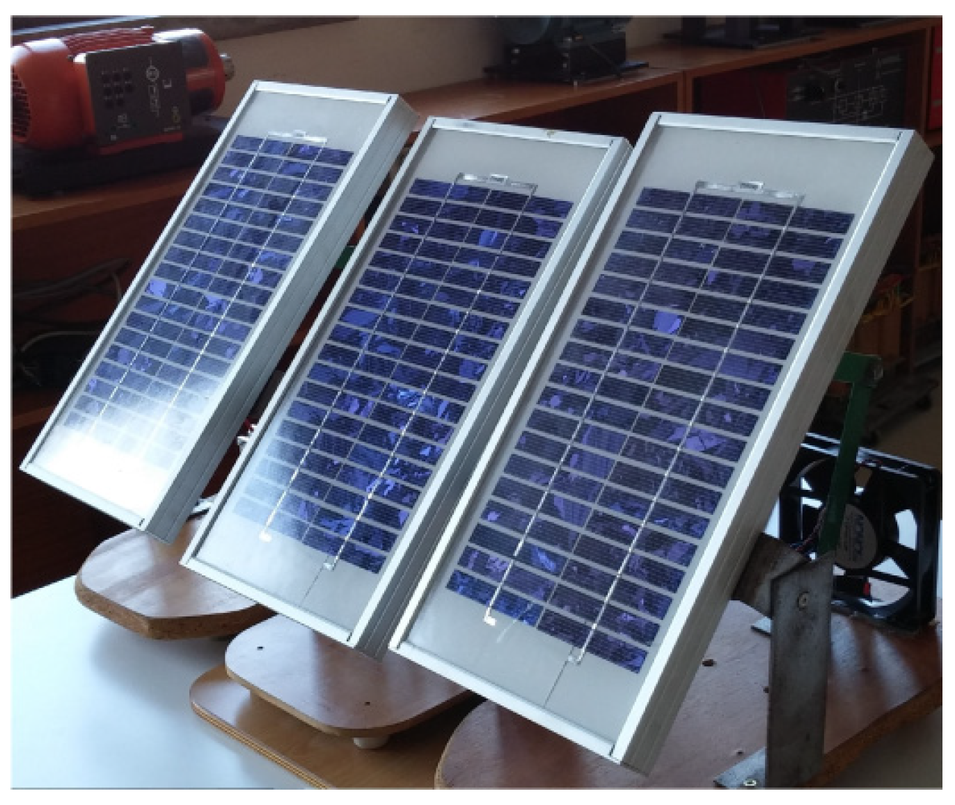
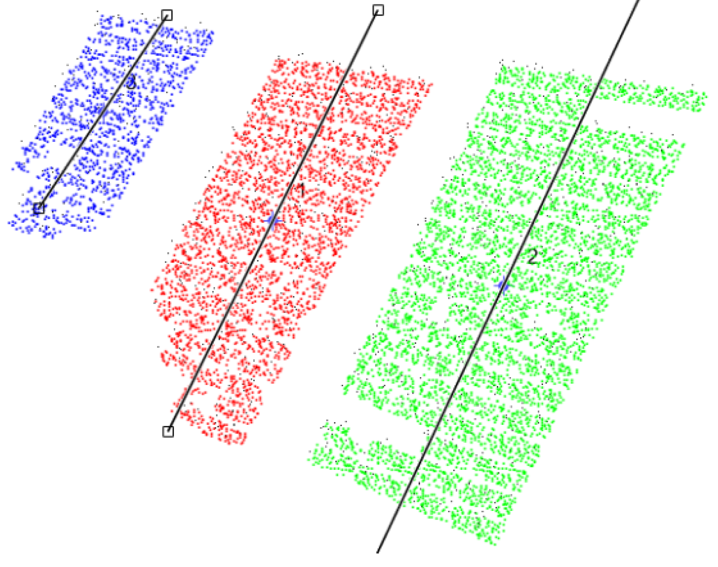
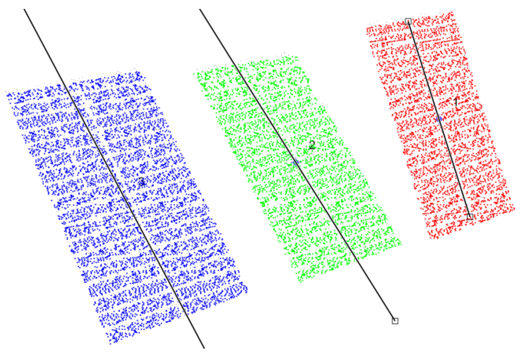
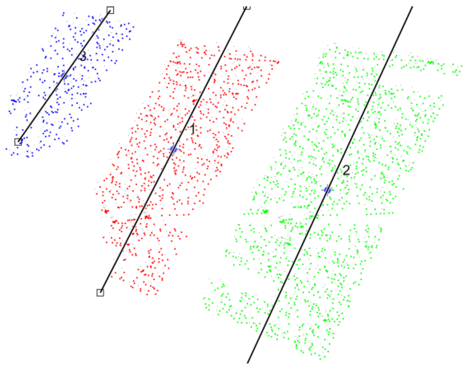
3.1. Trackers of the PV Panels with No Fault

The first case study used to verify the capability of the approach to identify the panels and their slopes, considers the condition in which all the trackers of the panels do not present any fault. In Figure 6, the image that was used for this test is presented. From this image, it is possible to see that all the panels present the same orientation indicating that there are no faults in the trackers. As referred previously, first the image processing was used to identify and isolate the PV panels that are inside the photograph. The result of this processing can be seen in Figure 7, in which it is possible to confirm that the panels were isolated from the rest of the image information. One of the aspects that can be seen by this figure is that some of the cells of the PV panel were not identified. This is due to the reflections that appear in PV modules. The orientation of each panel, θⁱ, is determined by the principal component of the points that belong to it. To assign each point to the correspondent panel the clustering algorithm described above was used (Equations (1) and (2)). Considering that three PV modules exist, three clusters, with the distance as a criterion, were then constructed. In Figure 8, the assignment of each cell points to a PV module and the correspondent orientation of the principal components are shown. Through this figure it is possible to see the attribution of each point to each panel through the application of the clustering process.

The results that were obtained regarding the orientation of the three PV modules, determined by the proposed method, are described in

Table 1. Module orientation and DI (situation in which there is not a fault in the trackers).

	PV Module 1	PV Module 2	PV Module 3
θi	61.5°	62.7°	58.3°
DI	0.37	1.03	1.40

. Analyzing the obtained values it is possible to see that the angles associated with the orientation of the PV panels are very similar. They are not exactly equal because in this case the orientations of the modules were made manually, and it was not possible to obtain a perfectly equal orientation. In this way, these angles indicate that there is not a fault in any of the trackers associated with the three PV panels. Although some cells of the PV panels were not identified due to reflections, the algorithm is still able to correctly detect their orientation.

In order to verify the automatic process to identify a fault, the average value of the angles must be obtained first. In this case, an average angle of 60.83° was obtained. In accordance with this it will be possible to determine the deviation index (DI). The angles and deviation indexes associated to each of the PV panels are presented in Table 1. From these values is possible to conclude that the threshold value must be higher than 1.40.

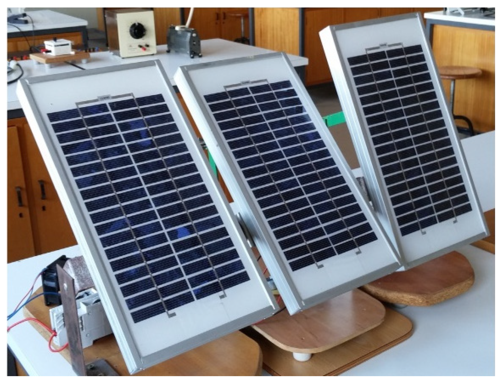
3.2. One of the Trackers with a Vertical Fault

The second case study is related to a condition in which there is a fault in one of the trackers. The image associated with this case study is presented in Figure 9. Verifying this photograph, it is possible to see that the PV module located on the right (PV Mod. 1) presents a different orientation when compared with the other two. The fault is associated only with the vertical axis of which the different orientation is related with that axis. Applying the image treatment to this figure, the identification of each of the three PV modules was obtained, as shown in Figure 10. Indeed, this figure shows that the image information that does not belong to the PV panels was removed. Regarding the step in which each of the points are assigned to the correspondent PV module, the corresponding result can be seen in Figure 11. This result shows the principal component obtained for each of the PV panels. Analyzing the resulting image, it is possible to see that the principal component follows the slope of the PV panels.

The computed values of the orientation of the three PV modules that were obtained by the proposed method are presented in

Table 2. Module orientation and DI (situation in which there is one tracker with a vertical fault).

	PV Module 1	PV Module 2	PV Module 3
θi	107.5°	121.0°	118.9°
DI	6.91	0.58	0.58

. Comparing the obtained slopes of the PV panels it is possible to confirm that the slope of the one located on the right (PV Module 1) stands out from the other two. Regarding the computed average angle to determine the deviation index (DI), a value of 119.95° was obtained in this case. In accordance with this value it is possible to obtain the deviation indexes, as shown in Table 2. Analyzing those values, it is clear that the PV panel with the fault in the tracker presents a much higher value. Moreover, comparing those values with the higher DI of the previous case (no fault), only the DI of the PV panel with the track under fault presents a higher value. Besides that, that value is much higher than the one of the previous case (6.91 to 1.40). So, even in situation of errors it is possible to define a threshold that must be slightly higher than the maximum DI value obtained for the normal situation.

3.3. One of the Trackers with a Horizontal Fault

A third case study with a different fault was also realized. This test is related to a fault in the PV panel located on the right (PV Module 3) and with a horizontal fault. In Figure 12, the image associated with this case study is presented, and it is possible to confirm the location and different orientation of the PV with the fault in the tracker. The identification of each of the three PV panels by the developed algorithm can be seen in Figure 13. In fact, that figure confirms the removal of the information that does not belong to the PV panels. The assignment of each point to the correspondent PV module and the correspondent principal component can be seen in Figure 14. This figure confirms that the points were correctly assigned to the PV modules and that the principal component follows the slope of each PV panel.

Regarding the obtained values of the proposed method for the orientation of the three PV modules, they can be seen in

Table 3. Module orientation and DI (situation in which there is a horizontal fault in one of the trackers).

	PV Mod. 1	PV Mod. 2	PV Mod. 3
θi	110.1°	106.0°	123.3°
DI	1.13	1.13	8.47

. Analyzing these values it is possible to see that the one with the different slope is the PV module related to the tracker fault (PV Module 3). This confirms the capability of the method to locate the panel that is attached to the tracker under fault. The average angle that is obtained from the method is 108.05°. With this value, the deviation indexes are determined, and it is possible to verify those values in Table 3. Analyzing the deviation index associated to each PV panel, it is possible to verify that only the one associated with the tracker with a fault presents a very different value. On the other hand, comparing these values with the higher DI of the test of no fault condition, it is possible to confirm that only the DI of the PV panel with a fault in the tracker presents a higher value showing the identification of this type of fault in an automatic way.

In the proposed method, one of the factors that influence the computational cost is the dimension of the matrix used in the PCA computation. In the presented paper, the effect of reducing the size of the matrix to calculate the orientation of the PV module was analyzed. To reduce the size of the matrix the down-sampling procedure was used in the data points that belong to the PV cells. The reduction of the processing time of the PCA computation with the down-sampling procedure is shown in

Table 4. Computation time of the PV modules using PCA.

Images	Computation Time [ms]
	1:40:N	1:160:N	1:240:N
Case 1	0.747	0.160	0.120
Case 2	0.792	0.187	0.110
Case 3	0.672	0.132	0.096

. Decreasing the matrix dimension with the data points of the PV cells, the obtained orientation maintain the correct values and the computational cost also decrease.

3.4. Comparison

To verify the characteristics of the proposed approach, a comparison with the pattern recognition method proposed by [36] was also performed. The first comparison was made for the case study, in which there is no fault in the trackers. This case study is interesting since it is possible to see that due to reflections part of the PV cells associated with PV module 3 does not appear. In this situation, the other approach was not able to detect the correct value. Instead of a value around 58°, it obtained a value of 21°. This shows that the proposed method is much more immune to problems like this, which is very important in this kind of application. Another test was performed, in which the slope of one PV module was measured manually with high precision. In

Table 5. Inclination of the PV module considering several methods.

	Manually	Method [36]	Proposed Method
θi	112.6	113.5	112.7

, the obtained values for the three methods are presented. Analyzing this table, it is possible to verify that the proposed method presents practically the same value as the one obtained manually. Regarding the method of [36], it gives an approximate value but with an appreciated error. The problem of the method [36] is that to give a very precise value it needs to perfectly identify all the cells of the PV panel, which typically is very difficult in this kind of application.

Through this comparison it was possible to verify the advantage of the proposed approach, namely since it can be used for images with reduced points and presents some immunity to incomplete parts of an object in an image.

4. Discussion

The developed image-processing algorithm based on the PCA was implemented to diagnose faults in solar trackers panels with two axes. Since the PCA is determined using the points that belong to the PV cells when partial occlusion in a panel occurs, there are the remaining points that allow the correct calculation of the slope. It is what happened in the first case study, where the left and middle panels had some reflection in their PV cells (Figure 6). In this situation, although the obtained slope values are not the same for the three panels, they are within the tolerance margin that allows for inferring that there is no fault in the trackers. It should be noted that in the three case studies the angular positioning of the panels was not performed with precision, thus justifying the differences in the values of slope obtained for panels that apparently appear to be completely aligned. The processing time of the proposed method depends on the number of PV cell points used in the PCA calculation. The computational time, when the down-sampling is higher than 1:40, is reduced when compared with the one obtained by the method presented in [36] which was 0.681 ms. Figure 15 and Figure 16 show the points in each panel, used in the principal component of each module, using a down-sampling of 1:160 and 1:240, respectively. It can be seen that the direction of the three panels in both situations are practically unchanged showing that even by sharply reducing the number of points used in the calculation of the PCA, the orientation obtained by the proposed method is quite the same. One aspect that was possible to verify, is that the proposed method is able to handle images that are incomplete due to reflections. This is an important aspect, since it was verified that in the other method used for the recognition of the PV panel, erratic slope values were obtained.

Another aspect is related with the implementation of this procedure in an automatic way in a large PV plant. So, regarding this aspect, there are several possibilities. However, a practical possibility is through the implementation of a structure in which a camera (with mobility capability) or cameras are strategically located in order to take a picture of all panels.

Regarding the angle that this procedure can detect with feasibility to detect any failure, the resolution depends of the defined threshold value. In this case, since the slope of the panels was implemented manually, there are some errors that do not appear in a real system. So, in a real system the angles of panels of the healthy trackers will practically present the same value, by which the resolution can be lower than 1 degree, or lower than 0.01 deviation index (DI). However, since this precision is not needed, one recording every 15 min is more than enough, and higher angles (or deviation indexes) are recommended. In these particular case studies, considering that in healthy conditions they do not have exactly the same slope, since they were aligned manually, there was a maximum error of 4.4 degrees, or under the point of view of the deviation index 1.40.

5. Conclusions

This paper focused on an algorithm to diagnose faults in solar tracker panels with two axes. This algorithm can be associated with a camera that acquires photographs. Thus, with the purpose of obtaining a fast diagnosis of a fault in the trackers where the PV modules are installed, a new method is proposed, using an artificial vision process. In this way, the identification of the fault is realized through a pattern recognition process applied to the PV modules’ photographs. The use of photographs for the detection of these types of faults presents an important advantage since it allows a fast fault detection ensuring maximum renewable energy production. On the other hand, this approach also means avoiding the acquisition of large amounts of data, as well as extra sensors. The new image processing approach uses principal component analysis (PCA) to process images. However, instead of using the PCA to reduce the data dimension, as is usual, in this case it was proposed to use it to determine the slope of an object. In this way, in the context of several PV modules, it will be possible to identify the PV module(s) with a different slope from the majority. Besides the identification of the PV modules and their slope in a photograph, a deviation index that can be used to discriminate the panel(s) under fault is also proposed. So, with the proposed approach, several benefits are obtained, such as, avoiding the use of a wide range of data and specific sensors, fast detection and reliability, even when there are incomplete parts of an object in an image. It was also possible to verify that the PCA enables the correct determination of the slopes of a PV panel even with down sampling. To test the proposed approach several case studies with and without fault trackers were used. A comparison with other method based on a pattern recognition approach was also realized. From this comparison, it was possible to conclude that the proposed approach obtains a more effective detection, even in a situation in which the images are incomplete due to reflections.

References

1. Soytaş, U.; Sarı, M. Handbook of Energy Economics; Taylor and Francis Group: Abingdon, UK, 2019; 620p. [Google Scholar]
2. Zhu, R.; Guo, W.; Gong, X. Short-Term Photovoltaic Power Output Prediction Based on k-Fold Cross-Validation and an Ensemble Model. Energies 2019, 12, 1220. [Google Scholar] [CrossRef] [Green Version]
3. Venkateswari, R.; Sreejith, S. Factors influencing the efficiency of photovoltaic system. Renew. Sustain. Energy Rev. 2019, 101, 376–394. [Google Scholar] [CrossRef]
4. Kishor, N.; Villalva, M.G.; Mohanty, S.R.; Ruppert, E. Modeling of PV module with consideration of environmental factors. In Proceedings of the IEEE PES Innovative Smart Grid Technologies Conference Europe, Gothenburg, Sweden, 11–13 October 2010; pp. 1–5. [Google Scholar]
5. Zhang, W.; Dang, H.; Simoes, R. A new solar power output prediction based on hybrid forecast engine and decomposition model. ISA Trans. 2018, 81, 313–326. [Google Scholar] [CrossRef] [PubMed]
6. Hafez, A.Z.; Soliman, A.; El-Metwally, K.A.; Ismail, I.M. Tilt and azimuth angles in solar energy applications—A review. Renew. Sustain. Energy Rev. 2017, 77, 147–168. [Google Scholar] [CrossRef]
7. Lee, C.-Y.; Chou, P.-C.; Chiang, C.-M.; Lin, C.-F. Sun tracking systems: A review. Sensors 2009, 9, 3875–3890. [Google Scholar] [CrossRef] [PubMed]
8. Mousazadeh, H.; Keyhani, A.; Javadi, A.; Mobli, H.; Abrinia, K.; Sharif, A. A review of principle and sun-tracking methods for maximizing solar systems output. Renew. Sustain. Energy Rev. 2019, 13, 1800–1818. [Google Scholar] [CrossRef]
9. Zhu, Y.; Liu, J.; Yang, X. Design and performance analysis of a solar tracking system with a novel single-axis tracking structure to maximize energy collection. Appl. Energy 2019, 264, 114647. [Google Scholar] [CrossRef]
10. Hafez, A.Z.; Yousef, A.M.; Harag, N.M. Solar tracking systems: Technologies and trackers drive types—A review. Renew. Sustain. Energy Rev. 2018, 91, 754–782. [Google Scholar] [CrossRef]
11. Zsiborács, H.; Baranyai, N.H.; Vincze, A.; Háber, I.; Weihs, P.; Oswald, S.; Gützer, C.; Pintér, G. Changes of Photovoltaic Performance as a Function of Positioning Relative to the Focus Points of a Concentrator PV Module: Case Study. Appl. Sci. 2019, 9, 3392. [Google Scholar] [CrossRef] [Green Version]
12. Zsiborács, H.; Baranyai, N.H.; Vincze, A.; Weihs, P.; Schreier, S.F.; Gützer, C.; Revesz, M.; Pintér, G. The Impacts of Tracking System Inaccuracy on CPV Module Power. Processes 2020, 8, 1278. [Google Scholar] [CrossRef]
13. Fathabadi, H. Comparative study between two novel sensorless and sensor based dual-axis solar trackers. Sol. Energy 2016, 138, 67–76. [Google Scholar] [CrossRef]
14. Sidek, M.H.M.; Azis, N.; Hasan, W.Z.W.; Ab Kadir, M.Z.A.; Shafie, S.; Radzi, M.A.M. Automated positioning dual-axis solar tracking system with precision elevation and azimuth angle control. Energy 2017, 124, 160–177. [Google Scholar] [CrossRef]
15. Iftikhar, H.; Sarquis, E.; Branco, P.J.C. Why Can Simple Operation and Maintenance (O&M) Practices in Large-Scale Grid-Connected PV Power Plants Play a Key Role in Improving Its Energy Output? Energies 2021, 14, 3798. [Google Scholar]
16. Dienst, S.; Schmidt, J.; Kuhne, S. Case Study: Condition Assessment of a Photovoltaic Power Plant using Change-Point Analysis. In Proceedings of the International Conference on Smart Grids and Green IT Systems (SMARTGREENS), Aachen, Germany, 9–10 May 2013; Volume 1, pp. 1–6. [Google Scholar]
17. Camargo, A.; Smith, J.S. Image pattern classification for the identification of disease causing agents in plants. Comput. Electron. Agric. 2009, 66, 121–125. [Google Scholar] [CrossRef]
18. Malayil, M.; Vedhanayagam, M. A novel image scaling based reversible watermarking scheme for secure medical image transmission. ISA Trans. 2021, 108, 269–281. [Google Scholar] [CrossRef] [PubMed]
19. Hofer, M.; Marana, A. Dental Biometrics: Human Identification. In Proceedings of the Dental Work Information XX Brazilian Symposium on Computer Graphics and Image Processing, Minas Gerais, Brazil, 7–10 October 2007; pp. 281–286. [Google Scholar]
20. Karimi, M.; Asemani, D. Surface defect detection in tiling Industries using digital image processing methods: Analysis and evaluation. ISA Trans. 2014, 53, 834–844. [Google Scholar] [CrossRef]
21. Asokan, A.; Anitha, J. Adaptive Cuckoo Search based optimal bilateral filtering for denoising of satellite images. ISA Trans. 2020, 100, 308–321. [Google Scholar] [CrossRef] [PubMed]
22. Martins, J.F.; Pires, V.F.; Amaral, T. Induction motor fault detection and diagnosis using a current state space pattern recognition. Pattern Recognit. Lett. 2011, 32, 321–328. [Google Scholar] [CrossRef]
23. Deabes, W.; Abdelrahman, M. A nonlinear fuzzy assisted image reconstruction algorithm for electrical capacitance tomography. ISA Trans. 2010, 49, 10–18. [Google Scholar] [CrossRef]
24. Kim, T.-H.; Cho, T.-H.; Moon, Y.S.; Park, S.H. Visual inspection system for the classification of solder joints. Pattern Recognit. 1999, 32, 565–575. [Google Scholar] [CrossRef]
25. Hajihosseini, P.; Anzehaee, M.M.; Behnam, B. Fault detection and isolation in the challenging Tennessee Eastman process by using image processing techniques. ISA Trans. 2018, 79, 137–146. [Google Scholar] [CrossRef] [PubMed]
26. Berenguel, M.; Rubio, F.R.; Valverde, A.; Lara, P.J.; Arahal, M.R.; Camacho, E.F.; Lopez, M. An artificial vision-based control system for automatic heliostat positioning offset correction in a central receiver solar power plant. Sol. Energy 2004, 76, 523–653. [Google Scholar] [CrossRef]
27. Camacho, E.F.; Berenguel, M.; Gallego, A.J. Control of thermal solar energy plants. J. Process Control 2014, 24, 332–340. [Google Scholar] [CrossRef]
28. Najera, Y.; Reed, D.R.; Grady, W.M. Image processing methods for predicting the time of cloud shadow arrivals to photovoltaic systems. In Proceedings of the 37th IEEE Photovoltaic Specialists Conference, Seattle, WA, USA, 19–24 June 2011; pp. 188–191. [Google Scholar]
29. Chu, Y.; Pedro, H.T.C.; Coimbra, C.F.M. Hybrid intra-hour DNI forecasts with sky image processing enhanced by stochastic learning. Sol. Energy 2013, 98, 592–603. [Google Scholar] [CrossRef]
30. Gallardo-Saavedra, S.; Hernández-Callejo, L.; Duque-Perez, O. Technological review of the instrumentation used in aerial thermographic inspection of photovoltaic plants. Renew. Sustain. Energy Rev. 2018, 93, 566–579. [Google Scholar] [CrossRef]
31. Simon, M.; Meyer, E.L. Detection and analysis of hot-spot formation in solar cells. Sol. Energy Mater. Sol. Cells 2010, 94, 106–113. [Google Scholar] [CrossRef]
32. Mahmoud, Y.; El-Saadany, E.F. A Novel MPPT Technique Based on an Image of PV Modules. IEEE Trans. Energy Convers. 2017, 32, 213–221. [Google Scholar] [CrossRef]
33. Lee, C.-D.; Huang, H.-C.; Yeh, H.-Y. The Development of Sun-Tracking System Using Image Processing. Sensors 2013, 13, 5448–5459. [Google Scholar] [CrossRef] [Green Version]
34. Jaffery, Z.A.; Dubey, A.K.; Haque, I.A. Scheme for predictive fault diagnosis in photo-voltaic modules using thermal imaging. Infrared Phys. Technol. 2017, 83, 182–187. [Google Scholar] [CrossRef]
35. Tsanakas, J.A.; Chrysostomou, D.; Botsaris, P.N.; Gasteratos, A. Fault diagnosis of photovoltaic modules through image processing and Canny edge detection on field thermographic measurements. Int. J. Sustain. Energy 2015, 34, 351–372. [Google Scholar] [CrossRef]
36. Amaral, T.G.; Pires, V.F. Fault Detection in Trackers for PV Systems Based on a Pattern Recognition Approach. Int. Trans. Electr. Energy Syst. 2019, 29, e2771. [Google Scholar] [CrossRef]
37. Moore, L.M.; Post, H.N. Five years of operating experience at a large, utility-scale photovoltaic generating plant. Prog. Photovolt. Res. Appl. 2008, 16, 249–259. [Google Scholar] [CrossRef]
38. Oozeki, T.; Yamada, T.; Otani, K.; Takashima, T.; Kato, K. An analysis of reliability in the early stages of photovoltaic systems in japan. Prog. Photovolt. Res. Appl. 2010, 18, 363–370. [Google Scholar] [CrossRef]
39. Papadakis, K.; Koutroulis, E.; Kalaitzakis, K. A server database system for remote monitoring and operational evaluation of renewable energy sources plants. Renew. Energy 2005, 30, 1649–1669. [Google Scholar] [CrossRef]
40. Arena, E.; Corsini, A.; Ferulano, R.; Iuvara, D.; Miele, E.S.; Celsi, L.R.; Sulieman, N.A.; Villari, M. Anomaly Detection in Photovoltaic Production Factories via Monte Carlo Pre-Processed Principal Component Analysis. Energies 2021, 14, 3951. [Google Scholar] [CrossRef]
41. Wang, Y.; Ma, X.; Qian, P. Wind Turbine Fault Detection and Identification Through PCA-Based Optimal Variable Selection. IEEE Trans. Sustain. Energy 2018, 9, 1627–1635. [Google Scholar] [CrossRef] [Green Version]
42. Zhang, S.; Tang, Q.; Lin, Y.; Tang, Y. Fault detection of feed water treatment process using PCA-WD with parameter optimization. ISA Trans. 2017, 68, 313–326. [Google Scholar] [CrossRef]
43. Pires, V.F.; Amaral, T.G.; Martins, J.F. Power Quality Disturbances Classification Using the 3-D Space Representation and PCA based Neuro-Fuzzy Approach. Expert Syst. Appl. 2011, 38, 11911–11917. [Google Scholar] [CrossRef]
44. Otsu, N. A threshold selection method from gray-level histogram. IEEE Trans. Syst. Man Cybern. 1978, 9, 62–66. [Google Scholar] [CrossRef] [Green Version]
45. Ballard, D.; Brown, C. Computer Vision; Prentice-Hall, Inc.: Englewood Clifs, NJ, USA, 1982. [Google Scholar]
46. Rohlf, F.J. 12 Single-link clustering algorithms. In Handbook of Statistics; Elsevier: Amsterdam, The Netherlands, 1982; Volume 2, pp. 267–284. [Google Scholar]
47. Pandit, S.; Gupta, S. A comparative study on distance measuring approaches for clustering. Int. J. Res. Comput. Sci. 2011, 2, 29–31. [Google Scholar] [CrossRef] [Green Version]
48. Race, A.M.; Steven, R.T.; Palmer, A.D.; Styles, I.B.; Bunch, J. Memory Efficient Principal Component Analysis for the Dimensionality Reduction of Large Mass Spectrometry Imaging Data Sets. Anal. Chem. 2013, 85, 3071–3078. [Google Scholar] [CrossRef]
49. Khatun, T. Measuring environmental degradation by using principal component analysis. Environ. Dev. Sustain. 2009, 11, 439–457. [Google Scholar] [CrossRef]
50. Cherkassky, V.; Mulier, F. Learning from Data; John Wiley & Sons, Inc.: New York, NY, USA, 1998. [Google Scholar]
51. Jolliffe, I.T. Principal Component Analysis; Springer: New York, NY, USA, 1986. [Google Scholar]
Figure 1. Solar panel with a dual-axis tracker.
Energies 14 07278 g001
Figure 2. Strategy proposed for the detection of a tracker fault, namely through the comparison of the slopes between the PV panels.
Energies 14 07278 g002
Figure 3. Main steps associated with the proposed approach.
Energies 14 07278 g003
Figure 4. Adopted cells for panel’s orientation.
Energies 14 07278 g004
Figure 5. Constructed matrix for PCA algorithm.
Energies 14 07278 g005
Figure 6. Photograph in which all the trackers of PV panels do not present any fault (no fault).
Energies 14 07278 g006
Figure 7. Isolation of the PV panels by image treatment (no fault).
Energies 14 07278 g007
Figure 8. Principal component associated to each module (situation in which there is not a fault in the trackers).
Energies 14 07278 g008
Figure 9. Photograph of the PV panels in which there is a vertical fault in the tracker of the right PV module.
Energies 14 07278 g009
Figure 10. Isolation of the PV panels by image treatment (situation in which there is a vertical fault in the tracker of the right PV module).
Energies 14 07278 g010
Figure 11. Principal component of each module (situation in which there is a vertical fault in the tracker of the right PV module).
Energies 14 07278 g011
Figure 12. Photograph of the PV panels in which there is a horizontal fault in the tracker of the right PV module.
Energies 14 07278 g012
Figure 13. Isolation of the PV panels by image treatment (situation in which there is a horizontal fault in the tracker of the right PV module).
Energies 14 07278 g013
Figure 14. Principal component of each module (situation in which there is a horizontal fault in the tracker of the right PV module).
Energies 14 07278 g014
Figure 15. Principal component of each module for the first case using a down-sampling of 1:160.
Energies 14 07278 g015
Figure 16. Principal component of each module for the first case using a down-sampling of 1:240.
Energies 14 07278 g016