Hybrid Forecast and Control Chain for Operation of Flexibility Assets in Micro-Grids

Abstract

Studies on forecasting and optimal exploitation of renewable resources (especially within microgrids) were already introduced in the past. However, in several research papers, the constraints regarding integration within real applications were relaxed, i.e., this kind of research provides impractical solutions, although they are very complex. In this paper, the computational components (such as photovoltaic and load forecasting, and resource scheduling and optimization) are brought together into a practical implementation, introducing an automated system through a chain of independent services aiming to allow forecasting, optimization, and control. Encountered challenges may provide a valuable indication to make ground with this design, especially in cases for which the trade-off between sophistication and available resources should be rather considered. The research work was conducted to identify the requirements for controlling a set of flexibility assets—namely, electrochemical battery storage system and electric car charging station—for a semicommercial use-case by minimizing the operational energy costs for the microgrid considering static and dynamic parameters of the assets.

1. Introduction

Commercial microgrids were increasingly developed for demonstration purposes in the last decade, with the aim to locally optimize energy use and offer increased reliability to commercial customers with sensitive operations [1]. The cost to reduce photovoltaic and battery systems, together with the variability and inherent uncertainty of electricity prices, increased the interest for such localized energy systems by commercial customers for business-as-usual operations, which may address reliability, whilst providing cash flow certainty and reducing overall environmental impact.

Microgrids are typically operated in Low Voltage (LV) in both grid-connected and islanded modes [2]. Such systems may combine controllable and uncontrollable loads, as well as dispatchable and renewable generation sources, while lately research also focused on multicarrier systems [3] and the integration of the electro-mobility ecosystem [4].

The operation of microgrid systems similar to Figure 1 was studied and evaluated using a variety of methods, from purely centralized methods [5] to distributed control approaches [6]. Extensive comparisons amongst the merits of each method were examined in [7]; however, the distinct characteristics of commercial microgrids, in terms of single ownership, are driving the prevalence of centralized and hierarchical architectures. In such control architectures, data are produced by field devices and transferred via concentrators/gateways through to central intelligence units or platforms that typically contain data processing, storage, applications stacks, and associated interfaces. The application stacks for commercial microgrids range from various user-defined needs (such as reporting and billing) and core control-related applications, which are critical because aiming to maximize the customers’ benefit. The main control-related applications are the forecasting and the optimization/scheduling functions of the microgrid energy management systems, whose requirements are driven by the business objectives and the revenue streams of the commercial microgrids application.

In essence, this paper aims to highlight the importance of optimal control for storage systems through the analysis and demonstration of a real use-case (as a generic example) where the investment in renewable assets (storage) alone does not necessarily yield desired impacts but would deliver inverse results, such as increasing energy cost payments. Based on this finding, the present work provides a suitable system design for performing continuous forecasting, scheduling, and dispatch of commercial microgrids with a variety of Distributed Energy Resources (DERs). Several state-of-the-art contributions (reported in Section 2) established robust methods: however, they focused either on standalone forecasting or optimization applications and may ignore real-world deployment requirements with relaxed computational and communication constraints. In contrast, this paper introduces a complete chain of decision-making (Section 3) by first leveraging an innovative hybrid deep learning approach engineered and trained on data coming from the field to forecast solar production and load consumption (Section 4), and then the hybrid optimization algorithm developed from scratch to instruct smart setpoints to field devices (Section 5), closing the loop between data monitoring/collection and device control. Presented forecasting and optimization approaches use open-source and freely available resources showing accurate results with a low computational cost. Section 6 presents the conclusion regarding the studies, designs, and implementations reported in the paper, setting the stage for actual validation and implementation, as well as future work.

2. State-of-the-Art Review and Related Work

2.1. Photovoltaic (PV) Forecasting

Solar PV forecasting techniques are primarily driven by the dynamic nature of solar irradiance and other relevant meteorological parameters that induce high levels of uncertainty. This dynamic nature leads to voltage and power fluctuations, with subsequent impact on the microgrids energy management. As such, PV power forecasting is considered essential not only for efficient planning and integration of PV systems in power grids, but also for the optimization of their day-to-day operation.

In the past 20 years, a wealth of PV power forecasting (PVPF) methods was developed, studied, and established, addressing the whole spectrum of forecasting time horizons, i.e., from ultra-short-term forecasting (seconds to minutes) to long-term forecasting (months to years). In the case of microgrids, and especially for those that highly depend on local PV generation and potentially incorporate flexibility assets (e.g., batteries) and have special demand needs such as EV charging, safe and cost-effective day-to-day operation is an optimization problem that highly depends on reliable PV and load forecasting. Due to the inherent localized generation of microgrids, a suitable PVPF model should be in place to respond to frequent and sudden weather changes (e.g., cloud formation) and, as such, addressing the short-term (ST) with a view of at least one day ahead. The actual temporal horizon of ST PVPF is generally between 30 and 360 min [8], although other studies extend this horizon to several hours or even up to a week [9] towards achieving more effective power plant scheduling and market-related actions.

In the algorithmic domain, many approaches were studied involving physical, statistical, artificial intelligence, ensemble, and hybrid models. Traditional statistical methods, namely, time-series based forecasting techniques, involve curve fitting, moving average (MA), and autoregressive models and purely depend on mathematical equations to extract insight from historical data. Established techniques are the Exponential Weighted Moving Average (EWMA) [10], the autoregressive moving average (ARMA) [11], the autoregressive integrated moving average (ARIMA) [12], with the latter being the most popular time series analysis technique for the short-term horizon, succeeding reportedly very close accuracy rate with Artificial Neural Network (ANN)-based models [13].

However, among this variety of approaches, machine learning techniques, and especially ANN, their derivative models such as Multiple Layer Perceptron Neural Network (MLPNN) [14], Recurrent Neural Network (RNN) [15], and Deep Neural Network (DNN) [16], currently comprise the state-of-the-art in neural networks, and their hybrid or combined forms hold the most promising accuracy results, especially in case of short and medium forecast horizons. Not linked with complex mathematical content and obscure physical representations, while achieving remarkable results, these methods became the most popular choice for relevant researchers and industrial practitioners.

Recent studies on optimum PVPF in microgrid environments highlight the benefits of complex ANN models. For the case of a PV power generation microgrid with plug-in EVs (PVEVM), the paper [17] shows that a combination of a preceding clustering process of training sets comprising of numerical weather predictions (NWP) with the use of Density Peak Optimized (DPK)-medoids as input to a generalized RNN, provides high accuracy forecasts for a 30-min window and day-ahead horizon. The proposed PVPF model can not only forecast with high accuracy on sunny days, but also exhibits high-accuracy forecasting performance under unstable weather conditions. Using normalized root mean square error (nRMSE) as a validation metric and comparison tool, the proposed method reports values between 2.89–6.61%, depending on the cluster to which the forecasting day belongs and the weather characteristics, prevailing over both Markov Chain (MC) and simple Generalized Regression Neural Network (GRNN) models.

On a similar study on optimal load dispatch of a community microgrid, [18] demonstrates the significant results of deep learning-based solar power and load forecasting for a 60-min window and day-ahead horizon. In this case, a deep recurrent neural network with long short-term memory units (DRNN-LSTM) model was developed to forecast aggregated power load and the PV power output in the community microgrid. That model, using schedule variables (hour, day, month), and weather variables (global horizontal radiation, and diffuse horizontal radiation) succeeded in reaching an RMSE of 7.54, Mean Absolute Error (MAE) of 4.37 and Mean Absolute Percentage Error (MAPE) of 15.87%, significantly prevailing over Support Vector Machine (SVM) and multilayer perception (MLP) models’ overall error methods.

In the same vein, artificial intelligence (AI) methods were evaluated on PVPF in the case of a residential smart microgrid based on Numerical Weather Prediction (NWP) [19]. A 10-layer ANN was developed. The model proves to be the most efficient and accurate one to forecast the hourly irradiance and generated power for the residential microgrid compared to Multi-Variable Regression (MVR) and support vector machine (SVM) approaches using MAPE and MSE criteria. Overall, the neural network model reached 99.3% accuracy for the irradiance forecast with only 2 outliers, and it reached 98.5% accuracy for the power generated with only 4 outliers.

2.2. Load Forecasting

Electric load forecasting is a process used to predict the power or energy needed to balance the supply and load demand given historical load and weather information, together with current and forecasted weather information [20]. Depending on the time zone of planning strategies, load forecasting can be divided into three categories: short-term load forecasting (1 h to 1 week ahead), medium-term forecasting (1 week to 1 year ahead), and long-term forecasting (longer than a year ahead of the time of demand). More recent studies introduced a fourth category, the very short-term forecasting used for load forecasting from seconds up to one day ahead [21]. For this study, specific focus was given to short term load forecasting.

For short-term forecasting, a variety of methods (which include the similar-day approach, various regression models, time series, neural networks, fuzzy logic and expert systems) were developed over the years [20]. Broadly these techniques are divided into parametric and nonparametric ones. The similar-day approach, which is based on historical data search for similar days within recent years, the various regression methods, and the stochastic time series, used for decades in fields such as economics and digital signal processing, are examples of the parametric (or statistical) techniques. These techniques, however, are not capable of forecasting abrupt environmental or social changes; hence, in recent years, nonparametric techniques, such as ANN, emerged. Research shows that hybrid neural networks with learning techniques such as Genetic Algorithms (GA), Particle Swarm Optimization (PSO), Bacterial Foraging Optimization (BFO), or with fuzzy logic such as Artificial Immune System (AIS) can improve performance in terms of accuracy, computational cost and time [22].

Load forecast errors can have large negative consequences for a system operation, as they can lead to substantially increased operating and maintenance costs, decreased reliability of power supply and delivery system, and incorrect decisions for future development [23]. Literature suggests that a load forecast error of 1% in terms of MAPE can translate into several hundred thousand dollars loss per GW peak [21] when, as suggested, the typical day-ahead load forecasting error for a medium-sized US utility with an annual peak of 1 GW–10 GW is around 3% [24].

In the case of microgrids, load forecasting requires a different approach as the aggregated consumption figure is several times smaller than in region-wide areas and the load curve presents higher variability, leading traditional methods to be unsuitable for direct application [19]. While most solutions for load forecasting in large areas suggest MAPEs of around 2% [21,24,25], GRNN, Radial Basis Function Neural Network (RBFNN) models applied in the city of Hong (following a microgrid approach) between 2008 and 2010 suggest a MAPE of around 15% [19].

A study performed in 2018 applied three classical approaches for short-term load forecasting methods widely used in large networks—Seasonal Autoregressive Integrated Moving Average with eXogenous variables (ARIMAX), ANN, and Wavelet Neural Networks (WNN)—to a microgrid application. Results show that the WNN-based model has the highest prediction accuracy followed by the seasonal ARIMAX and NN-based model. The peak load error of the forecasts by the WNN-based model is between −40% to +30% at all times (and between −15% to 5% for 50% of the time), much lower than the seasonal ARIMAX and NN-based models with errors between −80% to 75% [26] but also much higher than the accepted forecast errors on the load forecasting for large networks.

2.3. Scheduling and Optimization

In the present context, optimization is referred to as the best operation planning for flexible components, essentially formed by an objective function and a set of constraints. An objective function might be the total operation costs, the constraints can be the equipment ratings and the decision variables can be the charge-discharge set-points of battery systems. It is of notable importance to treat every optimization problem appropriately by choosing relevant solving procedures from both method and implementation perspectives.

In a scheduling problem—e.g., flexibility asset operation—aimed to maximize economic returns, the objective function versus scheduling table might take a nonconvex course, while, on the other hand, the solution space could practically be infinite. These can restrict methods to be used for optimization problem calculation [27]. In some works, evolutionary methods are investigated for solving this family of problems [28,29]. In [30], a greedy scheduling method is proposed, where the computational time is critical. The authors of [31] wisely distinct distant and near-future forecast and optimization to deal with uncertainties. Energy cost minimization is dealt with in [32], where cycles of charge-discharge are also optimized. Dynamic tariffs for energy are also included in various studies [33] to accommodate that emerging scheme. Using a storage system as a means of service for the system operator is addressed in [34] to support business opportunities for ancillary service market participants.

In several case studies, the optimization problem is solved by rough-and-ready commercial or open-source tools. These so-called solvers are optimized in terms of code execution, parallelism, and power consumption [35]. Based on available resources, one may implement a custom optimization algorithm with distributed computation approach [36]. In many real use-cases, the need for flexibility in problem-solving outweighs those benefits due to the complexity of the problem itself, or implementation constraints such as hardware, operating system, etc.

2.4. Summary from the State of the Art

The assessment of use-case and analysis of the state-of-the-art highlighted important facts to design an integrated chain of applications—mainly forecast and optimization—that can be assembled as the following:

• Hybrid long- and short-range forecast and optimization are needed to better exploit resources ahead-of-time and deal with uncertainties;
• It is necessary to reduce unnecessary complexity of the calculations where possible to make separate modules more flexible in terms of time and computation;
• Regressive model with and without recurrence units can handle long- and short-range forecasting, respectively;
• An evolutionary algorithm and a greedy one can handle long- and short-range optimizations, respectively.

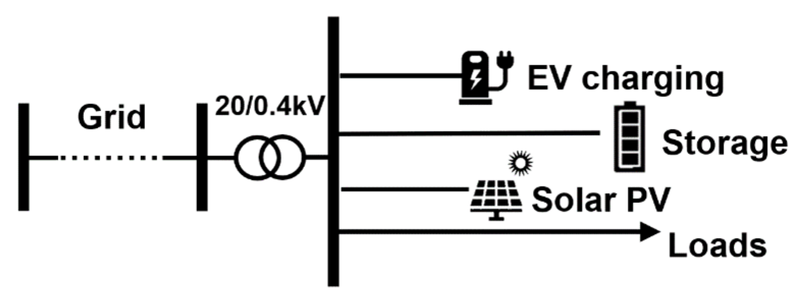
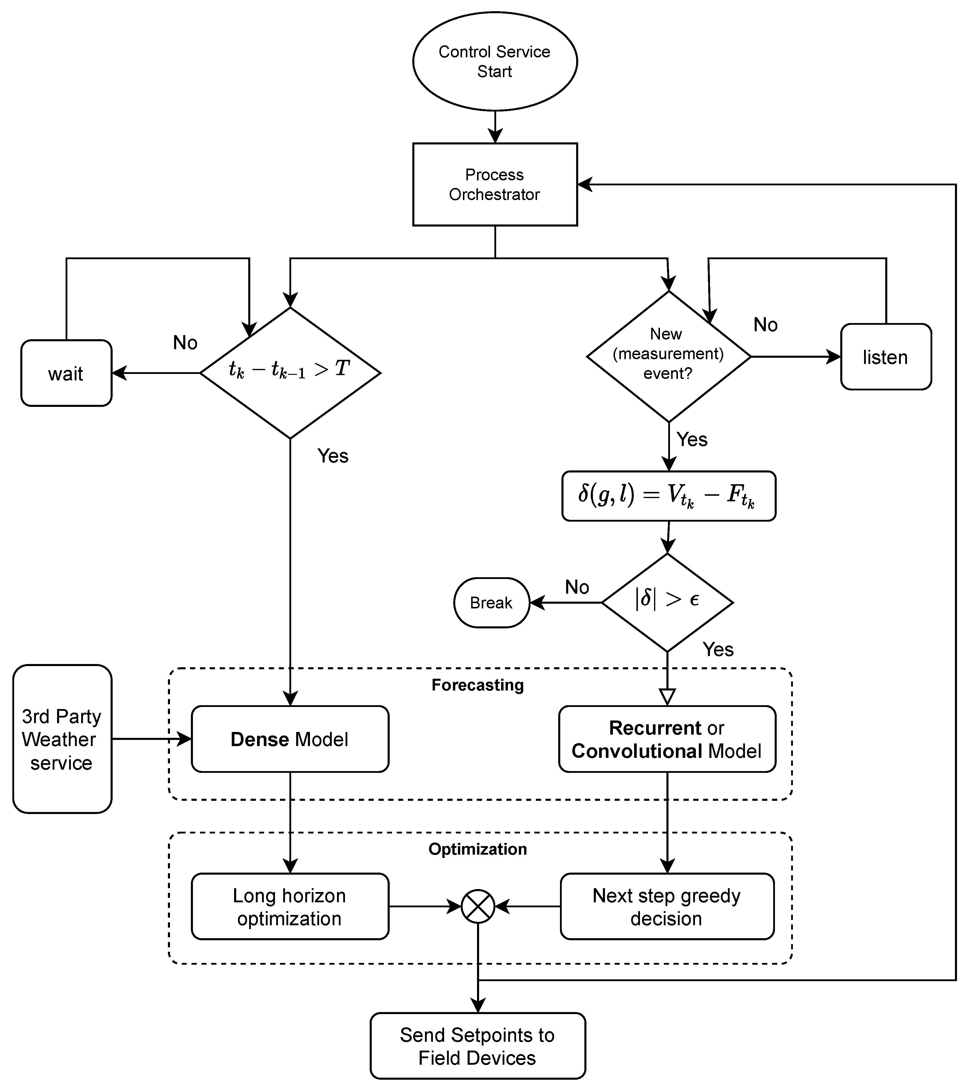
3. Management Process for Microgrid Operation

In many research efforts, the overall objective was to minimize operational energy costs for the microgrid considering static and dynamic parameters of its assets. The current work’s case falls into such kind of problem, and it is treated by designing two distinct modules of forecast and optimization.

The Forecast module is designed and developed as a hybrid forecast method by the integration of:

• A baseline regressive model to generate a forecast with long horizon H and big granularity, e.g., 48 h and 30 min, respectively.
• A recurrent model, for smaller time horizon and steps, e.g., 5 min ahead and 10 s steps, which gets activated upon errors between observed values and long-term forecast model.

The Optimization module follows the same hybrid approach since its input is fed directly from the forecast module. The current application is rendered with low complexity, where possible, to ease the integration within a chain of components from the physical field devices, gateways, and cloud service with continuous back and forth data flow. The hybrid approach is a combination of:

• Longer horizon and wider step optimization, matching baseline forecast (same time window and step) and triggered by that forecast updates. This optimization uses the meta-heuristics method as it deals with a complex problem, while it is less constrained in terms of calculation time.
• Spot decision-maker, namely greedy optimization, for very close actions, triggered by the recurrent forecast model.

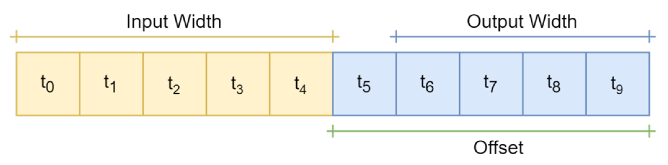
Figure 2 represents the control process of the full control chain, schematically.

The full-automatic control process is implemented as a web-service application that, once started, activates different routines, mainly Forecasting and Optimization Modules, alongside required connectors for devices and external services. The variables $t_c$ and $t_{k-1}$ represent current clock time and last activation time, respectively. At predefined interval T, e.g., half an hour, the process of long-horizon forecast (e.g., 48 h), and in turn, relevant optimization model, gets activated, and set-points are being sent for the next H hours. Due to the presence of noises (load and noncontrollable generation), a decoupled thread is placed to listening to the quasireal-time measurements from the field devices. If the difference between measurements $V_{t_k}$ and predicted values $F_{t_k}$ does not exceed certain defined error threshold $\epsilon$, the latest instructed set-points will be respected, otherwise a fast control chain (including a Recurrent forecast model and the consequent greedy optimization) quickly responds and overwrites the next(s) step’s set-point. Predictions and optimization models are described in detail in Section 4 and Section 5 respectively.

4. Forecasting

In the context of the current work, forecasting is an essential component for the optimal exploitation of renewable resources. It mainly includes prediction for two different variables: generation of Renewable Energy Sources (RES) and consumption coming from the noncontrollable load. The methodology used in this work is deepened in this section.

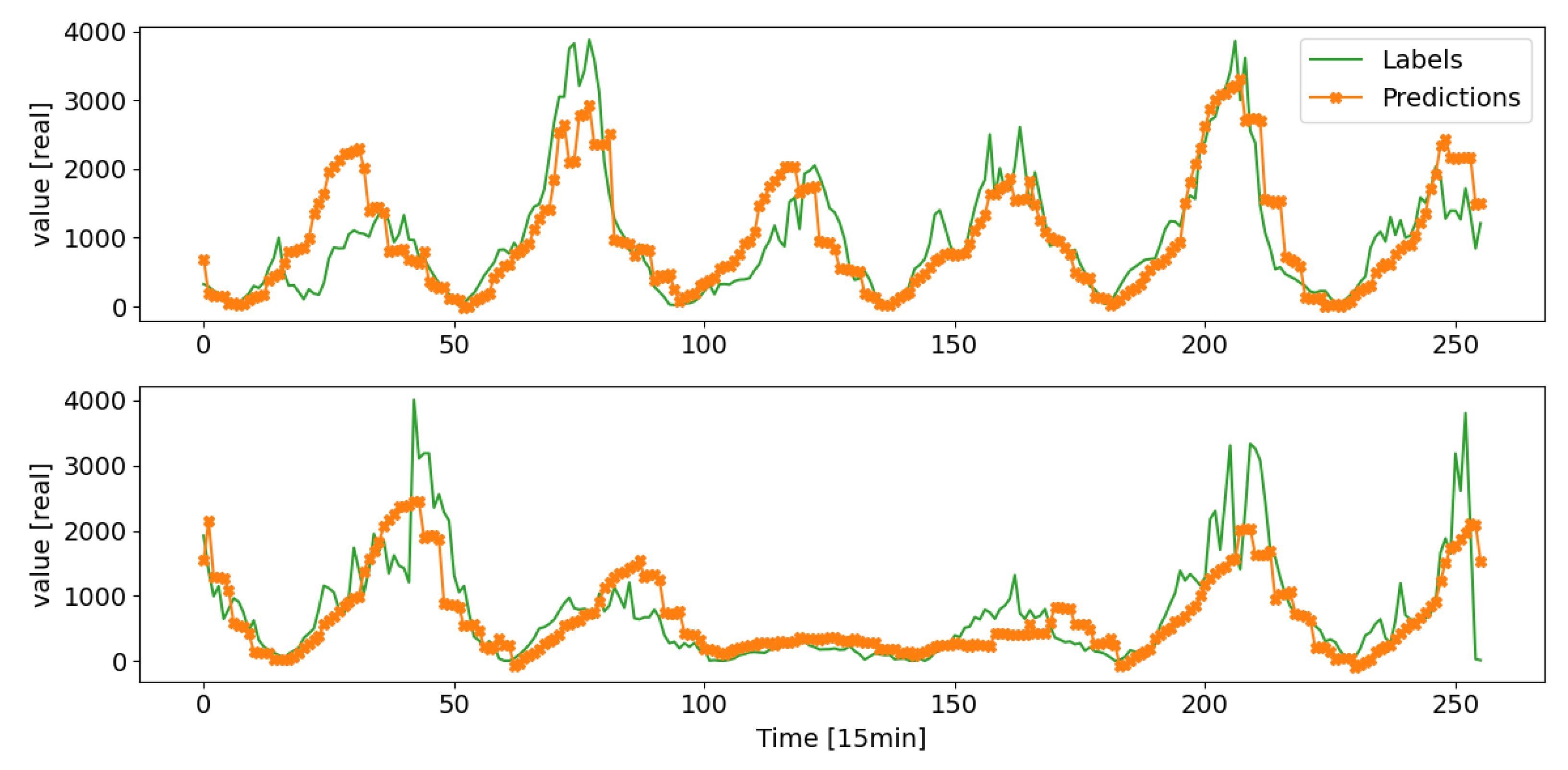
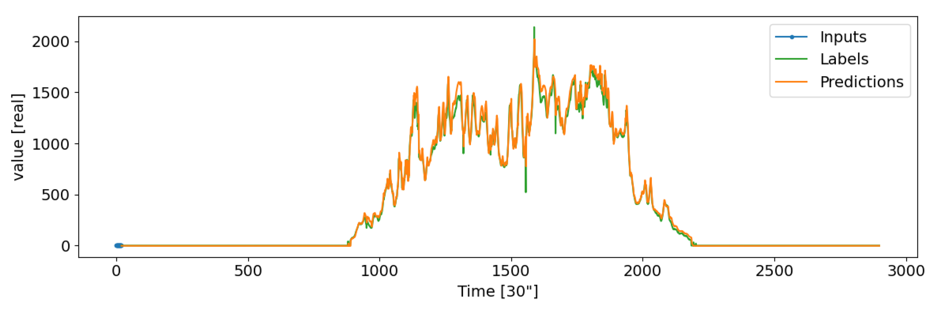
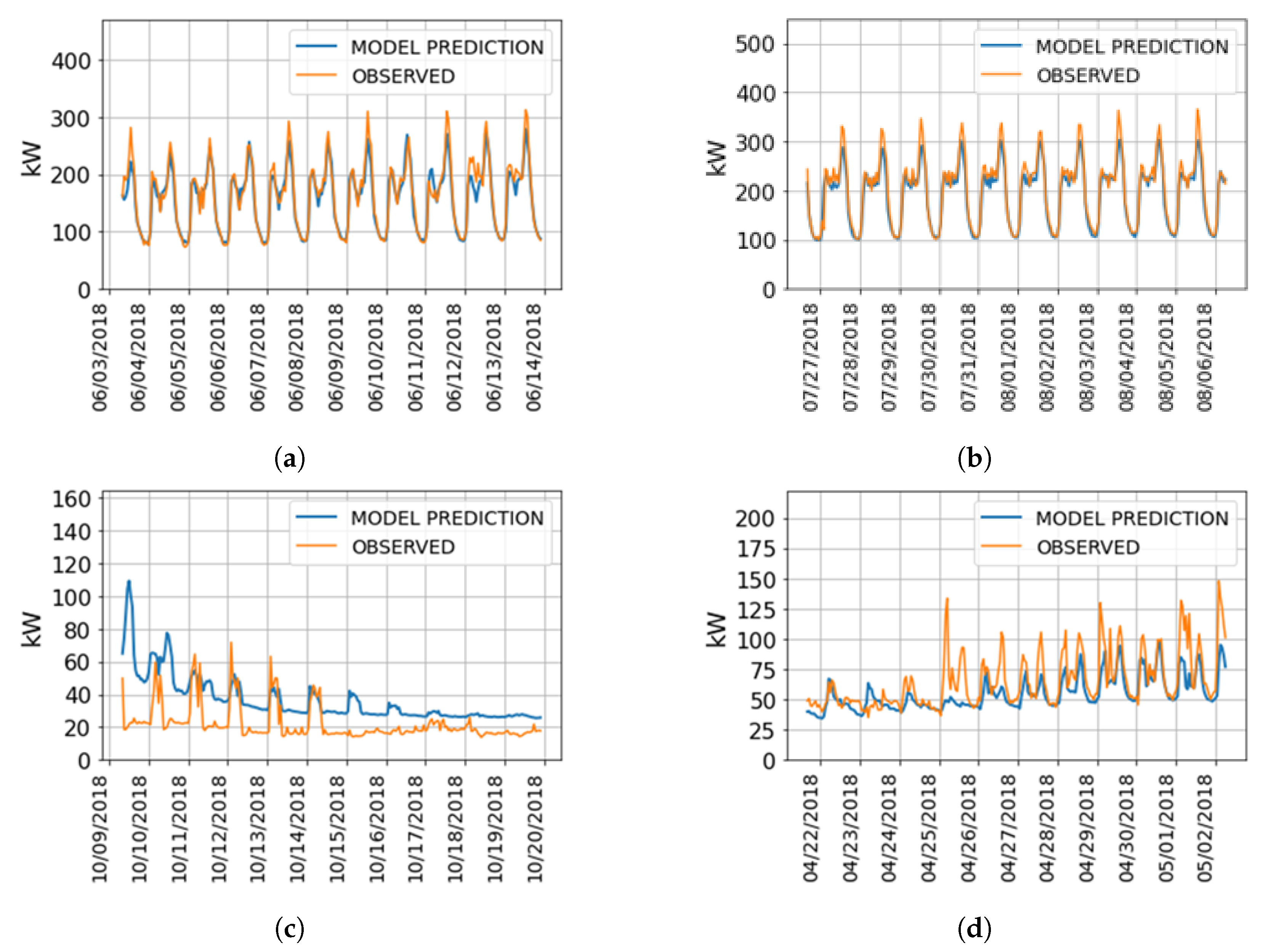
4.1. Renewable Generation

Since renewable generation is strictly correlated with the weather condition, and without an on-site weather station, a weather service capable of obtaining weather information and forecast is necessary. OpenWeatherMap (OpenWeatherMap One Call API: https://openweathermap.org/api, accessed on 20 October 2021) offers information about the current weather as well as the hourly weather forecast for 48 h. The former is used to populate the training dataset with a request to the API every 15 min, the latter becomes fundamental in the inference phase of the model. In addition to weather parameters, the model is fed with two synthetic sinusoids: one to represent the time of the day, and the second one represents the time of the year. A synthetic description of the dataset is provided in

Table 1. OpenWeatherMap data retrieved and used in model.

	Temperature	Feels Like	Pressure	Humidity	Dew Point	UVI	Clouds
id	temp	feels_like	pressure	humidity	dew_point	uvi	clouds
unit	°C	°C	hPa	%	°C	UV	%
mean	10.78	8.09	1017.47	75.0	6.27	1.03	42.15
std	4.73	5.71	9.15	15.35	5.20	1.26	34.04
min	−3.91	−12.84	979.0	15.0	−17.63	0.0	0.0
max	25.28	24.73	1047.0	100.0	20.83	4.25	100.0

.

Given that forecast accuracy is inversely proportional with the length of time window defined as output for the model and that the results depend directly on the precision of the weather provider, it was necessary to implement a short-term forecasting model to be used alongside the main model to correct the 48-h generation forecasting.

To implement this correction, an innovative approach was introduced as the “Hybrid Approach”.

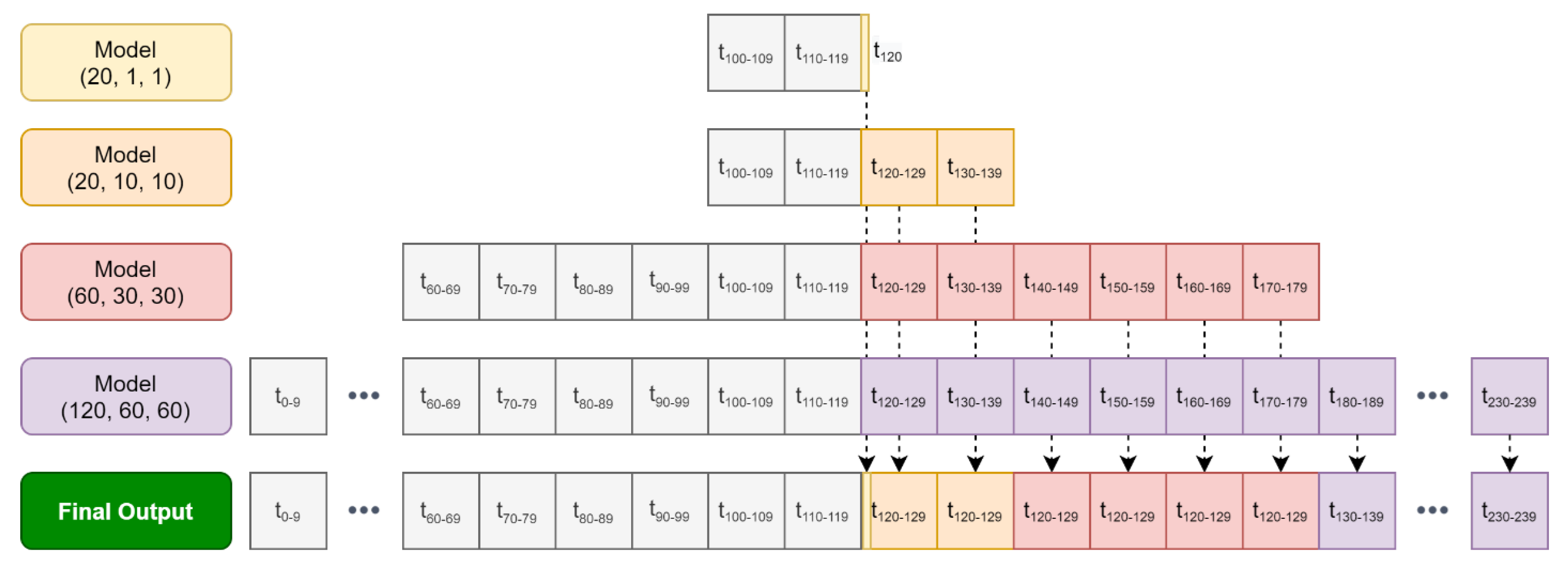
4.1.1. The Hybrid Approach

As the name suggests, the approach implemented exploits two different neural network architectures to enable two features that can be combined to predict renewable generation. The first component uses a Multilayer Neural Network to address long-term solar irradiance forecasting, while the second one exploits the potentiality of Recurrent Neural Network (RNN) and Convolutional Neural Network (CNN) to tackle short-term forecasting. The first component is always active, while the second one is triggered as a corrective factor whenever the difference between the long-term prediction and the current irradiation is greater than the selected threshold. This enables the field devices to take appropriate countermeasures against the uncertainty coming from weather forecasting.

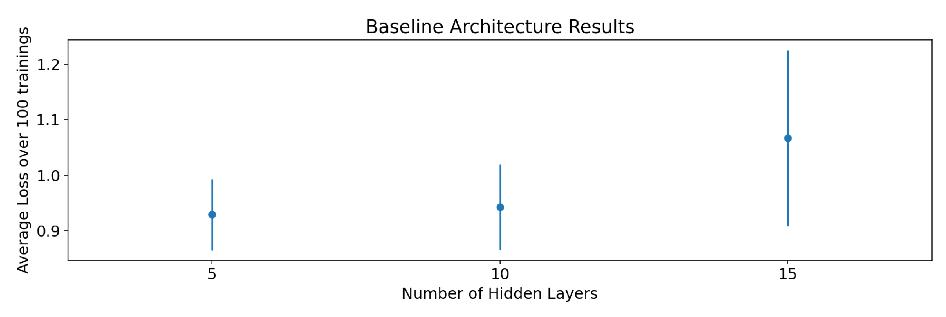
Long-Term Neural Network Design

The Neural Network architecture presented in Figure 3 is denominated Baseline because it generates the long-term forecasting which characterizes the first baseline for the approach. Indeed, it is used in the system to infer a single float value for sun irradiation for every hour in the 48-h weather forecasting provided by OpenWeatherMap in real-time. The Baseline Layer is the core part of the architecture and it is composed of a regular densely connected neural network layer with a specific hidden size and activation function, a layer for batch normalization and a dropout [37] one. To find the most appropriate architecture to use for this specific problem, an explorative grid-search was carried out to discover the best set of parameters capable of minimizing the loss in the test set (Mean Squared Error in this case) by using Adam [38] as an optimizer. The activation function selected for the training was the Rectified Linear Unit (ReLU). The hyperparameter tuning was set on the following factors:

• Baseline Layer Hidden Size - hidden_size $\in \{64,128,256,512\}$
• Number of Baseline Layers - $n\in \{5,10,15\}$
• Batch Size - batch_size $\in \{64,128,256,512\}$
• Dropout Rate - dropout_rate $\in \{0.1,0.3\}$

The hyperparameter-tuning process is composed of a training and validation phase for each epoch, with a final test phase to produce the final score for the specific run, given by the loss on the test set calculated using the network which yields the lowest validation error during the whole training. To pick this architecture, the best checkpoint during training is saved at the end of each epoch. An important help comes from the usage of Early stopping, a regularization technique for deep neural networks that breaks the training process when weights updates no longer yield improvements on the validation set.

To perform these experiments, 90% of the dataset is used for training and 10% for the testing phase. To correctly perform the validation phase for each epoch, 10% of the training dataset is exploited as the validation set.

Analyzing the results obtained from the first explorative grid search and some visual representations of the inference carried out on the test set for the most performing networks, it was noticeable that the networks with high hidden size, high dropout rate, and low batch size were the best performing ones. To make the final decision on the baseline architecture, all the hyperparameters were fixed except the number of hidden layers, and we performed 100 training experiments for each network to select the best one in terms of test loss and stability. The results reported in Figure 4, shows a better performance for the neural network with 5 hidden layers.

To conclude, the best performing architecture used to implement this component is the one with 5 layers, with a hidden size of 512, a dropout rate of 0.3, and a batch size in the training of 64. An example of the results obtained available in Figure 5.

Short-Term Neural Network Design

The second core component of the architecture is short-term forecasting. The candidate architectures chosen to implement this feature are:

• Long Short-Term Memory (LSTM) [39]: a key recurrent neural network architecture that outperformed vanilla RNNs by solving the vanishing gradient problems by the usage of additive components and forget gate activations;
• Gated Recurrent Unit (GRU) [40]: a type of recurrent neural network similar to an LSTM. The main difference is that it has only two gates (reset gate and update gate) and no output gate. Generally, it is easier and faster to train than the LSTM architecture.
• WaveNet [41]: it is a type of convolutional neural network developed in the context of the homonymous audio generative model. The architecture is based on dilated casual convolutions, which unveil a very large receptive field suitable to deal with long-range temporal dependencies.

Even if the structure of these three kinds of networks is fundamentally different, all training of these architectures was carried out by windowing the stream of real data of solar irradiation coming from the field with a granularity of 30 s. Setting aside input and output label width, a data window like the one shown in Figure 6 can be defined by a triplet of features: the input width (I), the output width (O) and the offset (F).

In the context of the experiments carried out, the following four windows were used:

• $I=20\left(10\min \right),O=1\left(30\mathrm{s}\right),F=1\left(30\mathrm{s}\right)$
• $I=20\left(10\min \right),O=10\left(5\min \right),F=10\left(5\min \right)$
• $I=60\left(30\min \right),O=30\left(15\min \right),F=30\left(15\min \right)$
• $I=120\left(60\min \right),O=60\left(30\min \right),F=60\left(30\min \right)$

The fundamental reason behind the usage of four different windows with models trained separately is the ability of networks to perform better in the short term. With a smaller output size, the optimization step of the neural network considers a smaller set to calculate gradients. On the contrary, with greater output size, there is more contribution to the calculation of the gradient. Therefore, on one hand, there is the need to have a short-term value of solar irradiation as close as possible to reality to properly correct excessive errors coming from the long-term forecasting; on the other hand, we would like not to be constrained by having forecasts only for the 30 s after receiving the last data from the field.

For this reason, even if the training of all networks was carried out independently, the outputs from each neural network are stacked on top of each other and precedence is given to values that come from a neural network with a smaller output size, which will override the output data coming from the neural networks with a larger but less accurate view. Figure 7 shows a graphical overview of the approach.

Even in this case, an explorative grid search was carried out to discover the best set of parameters. The loss used was Mean Absolute Error (MAE), the optimizer Adam with a learning rate equal to ${10}^{-3}$ and the activation function was the ReLU. The hyperparameter tuning was set on the following factors:

• LSTM and GRU
  • Layer Hidden Size - hidden_size $\in \{64,128,256\}$
  • Number of Layers - $\mathrm{n}\in \{1,2,3\}$
  • Dropout Rate - $d_r\in \{0.1,0.3\}$
• WaveNet
  • Layer Hidden Size - hidden_size $\in \{64,128,256\}$
  • Dropout Rate - $d_r\in \{0.1,0.3\}$

With $d_r$ standing for dropout rate. The number of hidden layers in the WaveNet architecture was not the object of the grid search because the dilation rate set of the convolutions was fixed to $\{1,2,4,8,16,32\}$.

The results are shown in

Table 2. Best Mean Absolute Error (MAE) reached in different grid searches.

Architecture	(20, 1, 1)	(20, 10, 10)	(60, 30, 30)	(120, 60, 60)
LSTM	0.11502	0.15777	0.24711	0.34303
GRU	0.11405	0.18512	0.26997	0.34971
WaveNet	0.12145	0.15497	0.25024	0.35345

. At first glance, LSTM achieves the best results in most of the architectures shown. However, the differences among the best loss reached for each architecture are in most cases negligible. In addition to this element, another factor that has to be taken into account in the evaluation of these modules is that CNNs like WaveNet are faster than RNNs in the training phase, while GRU has faster training than LSTM.

Given the fact that the differences among the losses are in most cases negligible and that CNNs are generally faster than RNNs in training, the WaveNet architecture was selected as the most suitable one for the experiments.

Figure 8 provides an example of results reported by asking recurrently the inference of the trained WaveNet (20, 1, 1) on a test data window with consecutive values of solar irradiance.

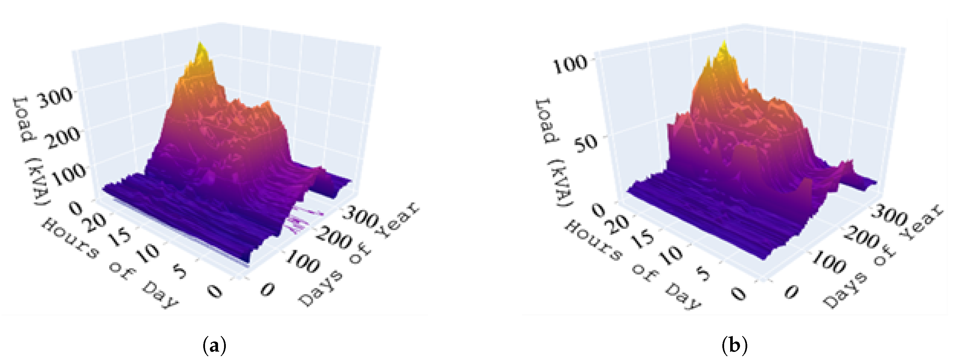
4.2. Load Consumption

Real energy consumption data were used in the present work to develop, train, and validate the proposed holistic forecasting and control methodology. The data come from a commercial customer connected to the Medium Voltage (MV), and its pattern is shown in Figure 9 over two consecutive years.

Main factors impacting on load (e.g., number of booked clients) are not available to the forecast model development, and therefore a direct correlation could be obtained from the recent evolution. Therefore, a recurrent model may fit this problem efficiently. Data properties of interest are identified as power, energy, and ambient temperature in different windows. Input data can be representations of power for the time slot in question in few past days:

$$F^I=\left\{a_{ik}|k\in \mathbb{K}\right\}$$

(1)

and total energy consumed in those days:

$$F^{II}=\left\{\sum _{j=-ik+1}^{-i\left(1+k\right)}{a}_j|k\in \mathbb{K}\right\}$$

(2)

with $n=24$ and $a=S$ (kVA). Also, ambient state variable such as temperature with $n=1$, $a=T$ (°C):

$$F^{III}=a_{ik}\left\{k|\in \left\{t^{+}-2,t^{+}-1,t^{+},t^{+}+1\right\}\right\}$$

(3)

The i is the sampling step size, e.g., $i=24$ in an hourly discretized dataset would mean state in the same hour one day before, and can be different for each feature. The set $\mathbb{K}$ consists of $\left\{0,1,2\dots ,t^{-}\right\}$ where $t^{-}$ is the lookback step. Temperature input is based on forecast data from 3rd party service, and in practice is not a representation from the past as $t^{+}$ represents the time shift or output step. The sampling number per variable can differ among them, and in that case for sake of matrix rendering, it is necessary to fill the lowest important steps (most distant ones) with the latest values but not zeros. The presented modeling is applied to load forecast for the $t^{+}\ge 1\left(h\right)$ window, while for $t^{+}<1\left(h\right)$ the forecast modeling comes from a recurrence approach similar to renewable generation forecast, with homogeneous samplings. Furthermore, input/output overwriting the near future forecast with relevant model follows the same logic reported in the renewable forecast section and Figure 6 and Figure 7. Input data are normalized according to Z score transformation following $z=\frac{\mathbf{x}-\mathit{\mu }\left(\mathit{x}\right)}{\mathit{\sigma }\left(\mathit{x}\right)}$, and architecture of the Load Forecasting ANN is composed of 2 hidden GRU layer with 32 and 64 neuron each, dropout of 0.2 at each layer, and ReLU as activation function. The output layer is implemented without – known also as Identity activation function.

The power consumption patterns are learned from presented recurrent networks as can be seen in Figure 10.

As one can see, in the example of 24 h models, forecasts are relatively acceptable except in transition seasons of consumption. Such errors are handled by the lower granularity models, and in fact, final results for the optimization module get already adjusted in real-time.

The overall performance of the Load Forecasting with the presented architecture is measured as MAE and it hits 0.133 and 0.0914 for 24 and 1 h ahead forecast, respectively.

5. Optimization-Based Control

The optimization-based control approach designed in this work considers the detailed price-related parameters of localized networks, as well as the technical specificity of hybrid inverter systems.

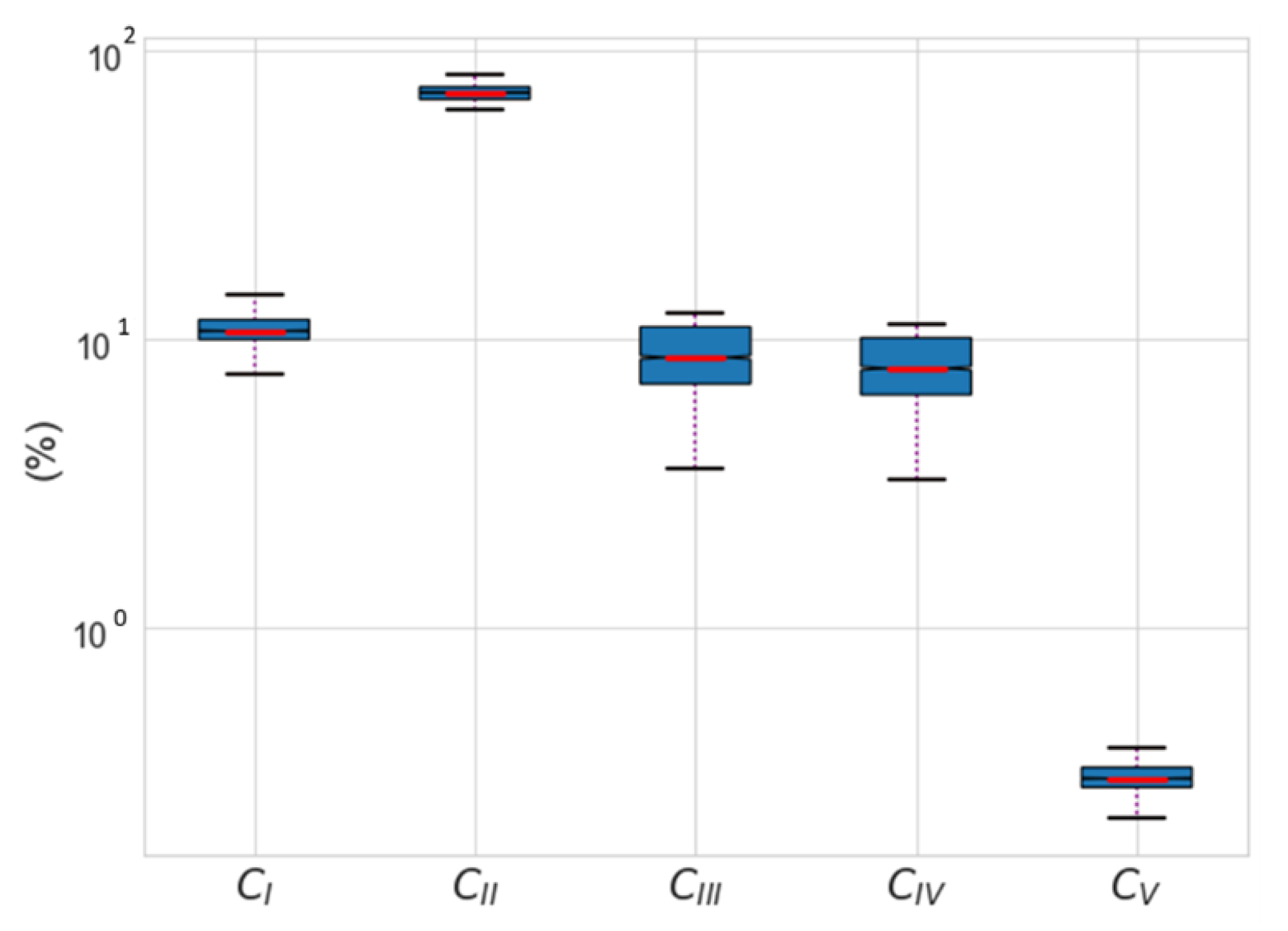
5.1. Price-Related Parameters

The electricity cost structure in the case study is composed of Q = 5 items:

• Base energy item: hourly energy cost with two-timing slots $t\in {\mathbb{T}}_1$ and $t\in {\mathbb{T}}_2$, and corresponding tariffs called Competitive Energy Tariffs (CET), namely ${\lambda }_{CE{T}_{S1}}$, ${\lambda }_{CE{T}_{S2}}$.

  $$C_I=\sum _{t\in {\mathbb{T}}_1}{E}_t\times {\lambda }_{CE{T}_{S1}}+\sum _{t\in {\mathbb{T}}_2}{E}_t\times {\lambda }_{CE{T}_{S2}}$$

  (4)
• Base power item: charge being activated for certain time slots (${\mathbb{T}}_{CPT}$) and applied to the peak power $S_t$ in that time-slot, called Competitive Power Tariffs (CPT). Where $t\in {\mathbb{T}}_{CPT}$ is the time slot between 7 a.m. and 11 p.m. on working days.

  $$C_{II}=\underset{t\in {\mathbb{T}}_{CPT}}{max}{S}_t\times {\lambda }_{CPT}$$

  (5)
• TSO Charge Power: or so-called Regulatory TSO Charge Power (TSOP) applied to the power term $S_t$ for a certain slot of time $t\in {\mathbb{T}}_{TSO}$, as a regulatory charge ${\lambda }_{TSO}$ for using the infrastructure of the transmission network.

  $$C_{III}=\underset{t\in {\mathbb{T}}_{TSO}}{max}{S}_t\times {\lambda }_{TSO}$$

  (6)
• DSO Charge Power: or so-called Regulatory DSO Charge Power (DSOP) applied to the power term $S_t$ for a certain slot of time ($t\in {\mathbb{T}}_{DSO}$), as a regulatory charges ${\lambda }_{DSO}$ for using the infrastructure of the distribution network.

  $$C_{IV}=\underset{t\in {\mathbb{T}}_{DSO}}{max}{S}_t\times {\lambda }_{DSO}$$

  (7)
• DSO Charge Energy: or so-called Regulatory DSO Charge Energy (DSOE) applied to the energy term $E_t$ for a certain slot of time ($t\in {\mathbb{T}}_1$), as a sort of regulatory charges ${\lambda }_{DSOE}$ for using the infrastructure of the distribution network. Time slots coincide with the same as in first item.

  $$C_V=\sum _{t\in {\mathbb{T}}_1}{E}_t\times {\lambda }_{DSOE}$$

  (8)

The time slots are enclosed in daily frames, and thus do not carry values among days (however, energy does carry quantities along days, so to solve the problem, the horizon gets extended, as will be explained in the optimization section), and these terms make up the final payment charge, in monthly fashions.

$$C=\sum _{i=1}^Q{C}_i$$

(9)

This objective function is directly affected by the applied tariffs. Figure 11 presents these contributions under various circumstances (different days and seasons, various levels of power generation and consumption); item II outweighs other terms due to its heavy payment charge.

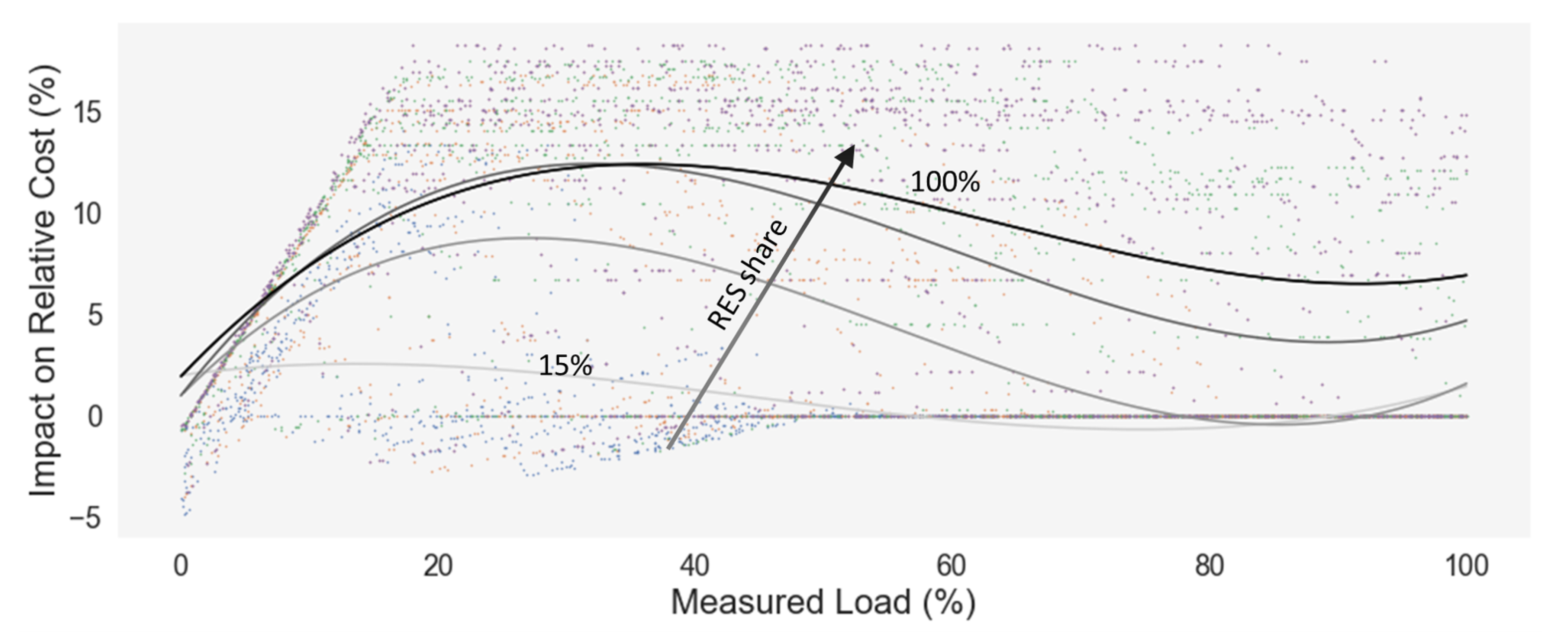
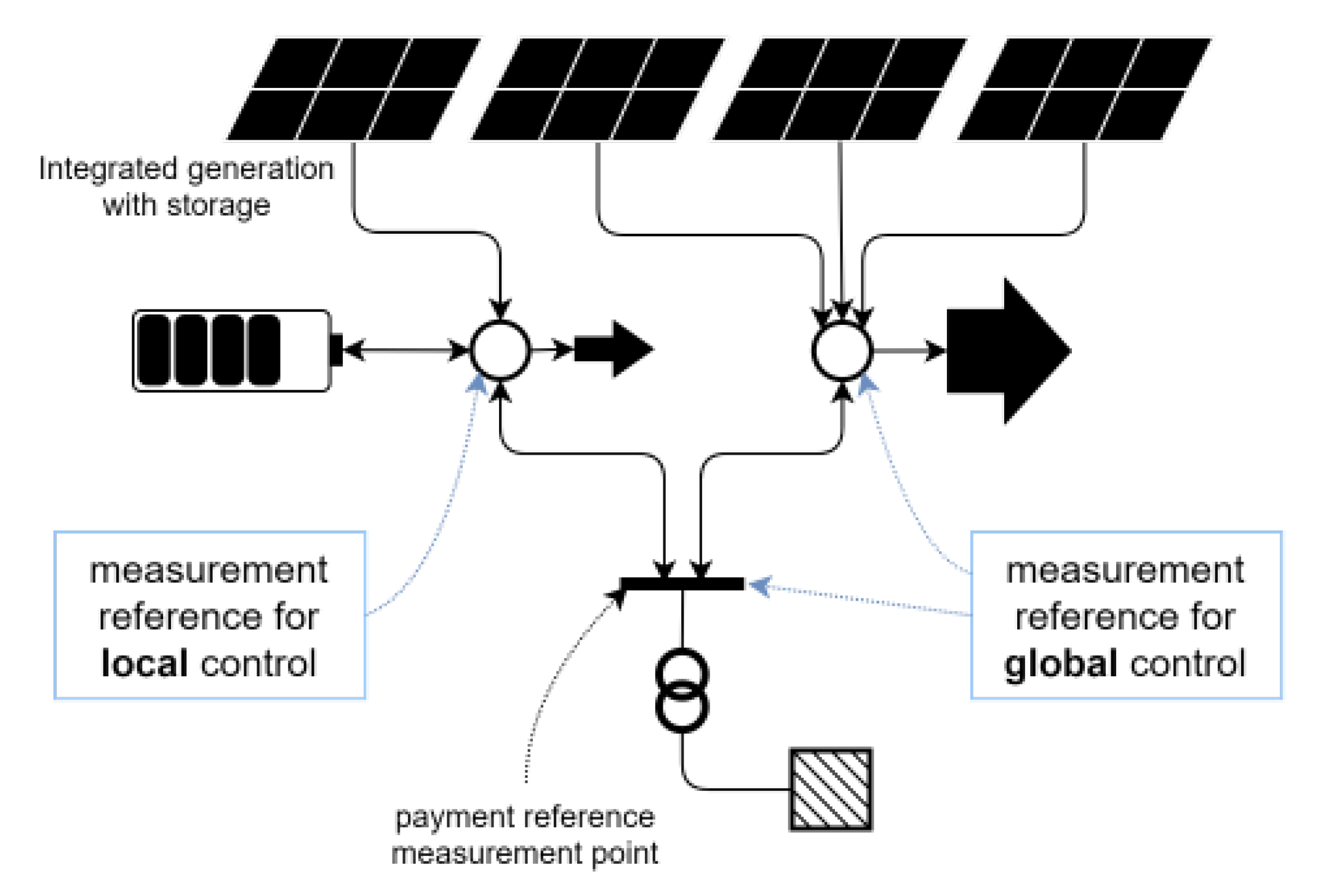
5.2. Localized Control Considerations

Classic control approach of flexible components, often established by the manufacturers as the default operation mode, might be following simple dummy/hysteresis/greedy decision process, based on local measurement of few variables for current time step and considering next clock action. This could be sufficient for some cases but could reduce the overall return of a flexibility system in others. In this case study, such control would even penalize the cost function, due to nonlinearity, as can be seen in Figure 12, where the horizontal axis represents the integrated portion of total load in the control process (say hybrid inverter’s load interface) and the vertical axis shows the relative difference between the total cost in cases with and without the storage system. The extreme case would raise the total cost by more than 15%, while in some cases can reduce it to 5%.

The intuitive reason is simply that energy consumption does not make up the main payment quote but the Base power item, which is active in midday (high photovoltaics production), and based on how much consumption is flown through local measurement point (in other words how the assets are configured according to the scheme shown in Figure 13), the dummy control would store the power rather than release it to the rest of the system which is a reference to total energy cost, as a whole. That said, a control method with a global vision is necessary.

Implementation of such necessity normally requires bypassing local control—run as inverter’s firmware—with notable sampling frequency and use external set-points via available interface, e.g., Modbus [42]. However, it is of importance to consider this approach makes the local control system blind, hence an accurate logic must be in place to cope with quasireal-time noises.

Advanced control methods group a wider range of variables enabling time-domain applications to handle the energy flow optimally for determined time horizons. Such an application could be highly relying on forecasts of state variables along considered time window, which might be uncontrollable loads, intermittent RES generation, dynamic prices if applied, etc. The latter mentioned time-series variables contain a higher range of variation as the aggregation level decreases. Although the optimization module was designed as a generic algorithm, the focus in the specific use case is to minimize energy cost subjected to a complex and non-convex formula with time-based elements as presented in Section 5.1.

5.3. Proposed Method

The optimization process responds to the relevant forecast submodule, meaning that for the H hours ahead battery system scheduling, an evolutionary method—namely Ant Colony Optimisation (ACO)— solves the problems, as it can return the results in a reasonable calculation time. In the following sections, an implementation of the classic ACO approach for battery system management is described, and furthermore, an extension is presented to accelerate calculations. Thereafter, the used Greedy logic for near steps ahead (corrective submodule) is reported.

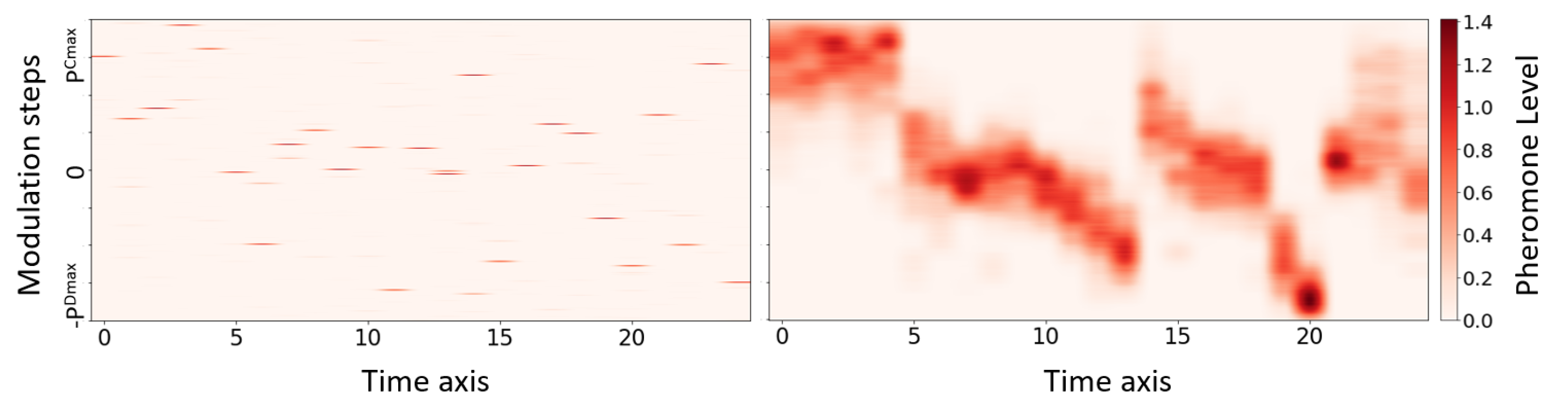
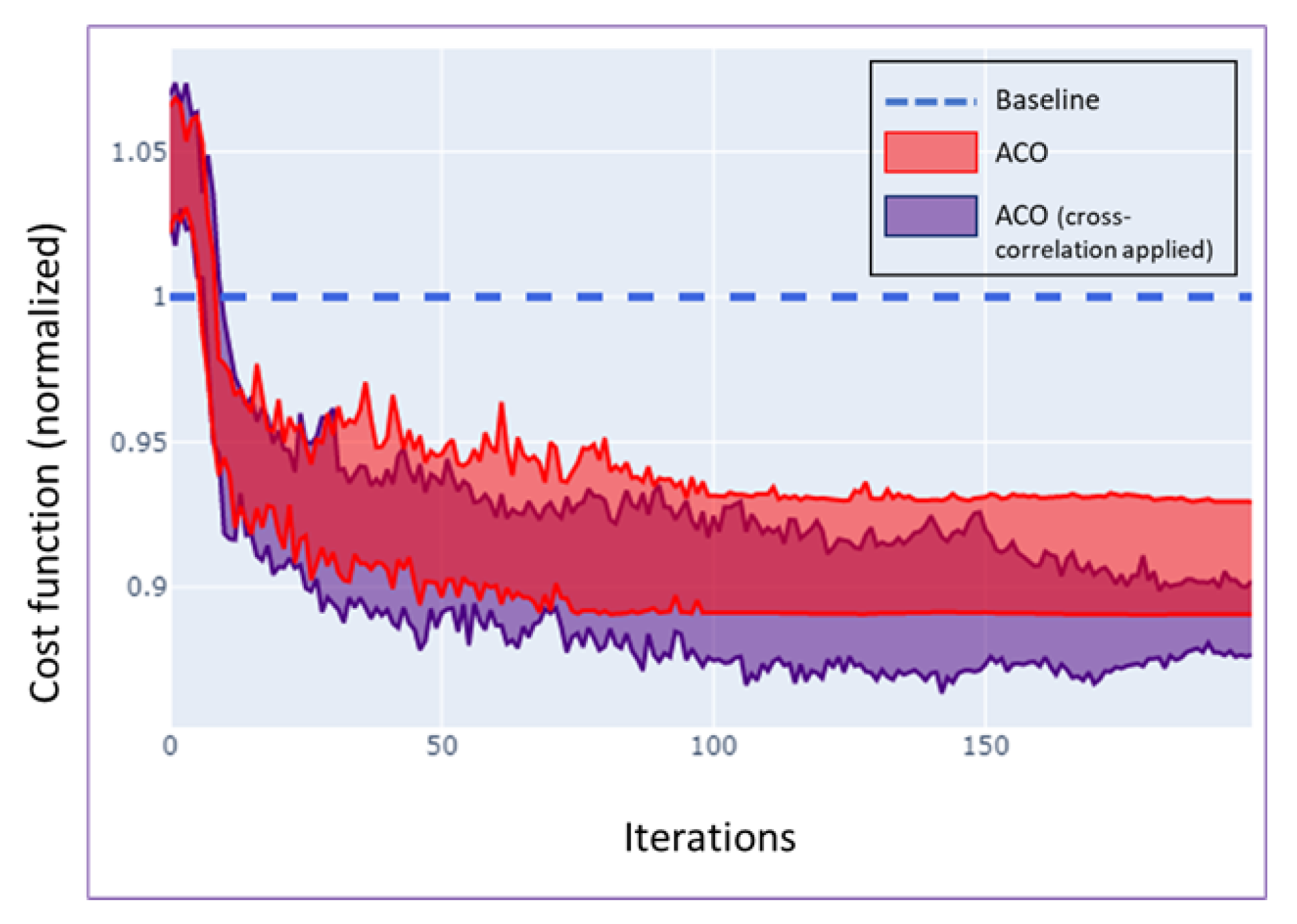
5.3.1. ACO for Smart Storage System Management

The scheduling problem along the considered time horizon H and the total number of modulation steps M could be managed as a discrete search space with the size of $M\times H$, rendered as a matrix with certain adjacency meaning. Let’s create such a matrix as probability distribution (pheromone) matrix and denote it by $\mathit{\chi }$, initialized with identical nonzero values. Pheromone matrix indicates possible best routes at each step, from each state.

It is of major importance to set up appropriate Depth of Discharge (DoD) to guarantee efficient lifespan for battery cells [43]. This consideration is in tune with global constraints such as State of Charge (SoC), maximum (${\mathrm{SoC}}_{\max }$) and minimum (${\mathrm{SoC}}_{\min }$) values. Arrangement of battery cells and corresponding power converter impose maximum power limit in charge and discharge states, ${\Delta E}_{max}^{+}$ and ${\Delta E}_{max}^{-}$, respectively. The latter two variables plus the capacity of the battery $E^{max}$ define the physical system’s constraints.

Power modulation steps can be defined as the following:

$$p=\left\{r:r={\Delta E}_{max}^{-}+{\Delta E}_{min}\times j,j\in \mathit{x}|r\le E^{max}\right\}$$

(10)

where minimum discretized power modulation is set to ${\Delta E}_{min}$ by problem definition. In fact, often ${\Delta E}_{min}$ is the known variable hence M will be determined accordingly. Auxiliary index vector for modulations, $\mathit{x}=\{1,2,\dots ,M\}$ will be used for sake of clarity.

Time axis (matrix columns), is defined similarly with selected minimum step size h, from Non-negative Natural Numbers ${\mathbb{N}}_0$ (including zero):

$$t=\left\{c:c=h\times j|j\in {\mathbb{N}}_0,j\le H\right\}$$

(11)

Generic ACO search basically follows the following steps:

• From certain state $S_0$, a group of artificial ants with a population of $N_A$ individuals start exploring the search space towards the end of a single path, according to the pheromones left on the route, but also the quality of next states. This forms a single solution.
• Evaluation of the found solution and associate it with a pheromone level, to be left on the path.
• Add the pheromone which is directly proportional with solution goodness on the traveled path.
• Apply evaporation rule, to balance the chances to select other routes, to avoid getting stuck in local optima.
• Repeating step 1 until a stop criterion is met.

For the current problem, the states can be considered as storage SoC or power modulation level along time horizon, to generate arbitrary solutions and evaluate them. The latter one is implemented in the present work. The search path starts in accordance with the $So{C}_0$ and proceeds respecting local constraints, at each time step:

$$-p_t^{\left(D_{max}\right)}\le p_t\le p_t^{\left(C_{max}\right)}$$

(12)

where maximum charge and discharge power modulation at step t, $p_t^{\left(C_{max}\right)}$ and $p_t^{\left(D_{max}\right)}$ respectively are defined as follows:

$$p_t^{\left(D_{max}\right)}=So{C}_{t-1}-max(So{C}_{min},So{C}_{t-1}-\Delta E_{max}^{-})$$

(13)

$$p_t^{\left(C_{max}\right)}=min(So{C}_{max},So{C}_{t-1}+\Delta E_{max}^{+})-So{C}_{t-1}$$

(14)

This defines available selections (next states) for the time step t as follows:

$$S=\left\{s\in x|p_t^{\left(D_{max}\right)}\le s\le p_t^{\left(C_{max}\right)}\right\}$$

(15)

Thereafter, the pheromone level for these states together with their quality is being used for making a selection for the current state. Selected states are stored in a temporary vector, and ${\mathrm{SoC}}_t$ will be updated according to the selection made:

$$So{C}_t=So{C}_{t-1}+p_t\times {\eta }^{sgn\left(p_t\right)}$$

(16)

$\eta$ is defined as the storage system overall efficiency. After each artificial ant finished its route with a predefined length, a single solution in terms of power is formed and can be evaluated by applying it to the predicted (aggregated) load profile.

An additional term can be used to control storage system usage, given that in some time slots battery storage could be charging and then discharging with no impact on the objective function. The additional term can make up a usage cost for storage; thus if no benefit is gained, it remains in idle state or last state, rather than completing the cycles when not necessary. One approach being tried is to add the following as storage usage cost to the overall term:

$${\lambda }_b={\left(\sqrt{\frac{1}{H}\sum _{t=0}^H{\delta }_t^{\left(j\right)}-{\mu }^{\left(j\right)}}\right)}^2$$

(17)

where ${\delta }_t^{\left(j\right)}$ is representing the first derivative of power modulation along the time axis for the solution j, and the ${\mu }^{\left(j\right)}$ is the average value of the latter expression.

Another approach is to include the cost of battery usage directly in the probability distribution formula used for selecting the next action in the classic ACO method:

$$P_{s,t}=\frac{{\tau }_{i,t}^{\alpha }\times K_{i,t}^{\beta }}{{\sum }_{i\in S}({\tau }_{i,t}^{\alpha }\times K_{i,t}^{\beta })}$$

(18)

The ${\tau }_{s,t}$ represents the pheromone matrix’ element for transient from state $t-1$ to t, for a certain state s. The $K_{s,t}$ indicated the quality of state s at step t. This quality is assigned to the battery usage cost, and it is simply set to:

$$K_{s,t}=\left\{\begin{array}{cc}\frac{1}{\nu !},\hfill & s=0\hfill \\ \frac{1}{(\nu +1)!},\hfill & \mathrm{otherwise}\hfill \end{array}\right.$$

(19)

With $\nu$ as an arbitrary constant. The exponents $\alpha$ and $\beta$ weigh two terms in overall expression. In the current application, clearly, the first term related to pheromone must be dominant. The $s_t$, next state of storage therefore is selected according to the considered probability distribution $P_{S,t}$.

Due to the introduction of the battery usage cost term, it is important to extend the solving horizon, simply because the optimization solver would take advantage of low price after peak hours if it made a better return.

Given the nonlinearity of the problem, pheromone level calculation needs rather to complete a single path or so-called solution $\varphi \left(j\right)$, then evaluating it keeping the baseline cost $C^{*}$ (i.e., the cost calculated on the basis of forecasts, in absence of flexibility) as a benchmark reference, and this obtains directly pheromone level:

$${\tau }_{s,t}^{\left(j\right)}=\left\{\begin{array}{cc}{l}_r(C^{*}-C_{\varphi \left(j\right)}),\hfill & C^{*}>C_{\varphi \left(j\right)}\hfill \\ 0,\hfill & \mathrm{otherwise}\hfill \end{array}\right.$$

(20)

The $l_r$ stands for an arbitrary rate for updates, that can be estimated initially, then optimized with a couple of iterations-inspections.

The $\varphi \left(j\right)$ is obtained by first applying the solution found to the non-controllable state variables i.e., apparent power consumption and generation, both as predicted time series, then calculating through the same cost equations C. In practice, the process is divided into several epochs $N_E$; at each, $N_A$ ants explore the search space without updating pheromones. Instead, they deposit that pheromone on an auxiliary matrix ${\mathit{\chi }}_{\mathrm{epoch}}$, which then would be used to update the pheromone matrix $\mathit{\chi }$.

$${\mathit{\chi }}_{\mathrm{epoch}}=\sum _{j=1}^{N_A}{\tau }_{s,t}^{\left(j\right)}$$

(21)

Evaporation emulation is basically applied by the following:

$$\mathit{\chi }=\left(1-\rho \right)\mathit{\chi }+{\mathit{\chi }}_{epoch}$$

(22)

These parameters of the calculation such as $N_E$, $N_A$, $\rho$, $l_r$ could be selected based on the complexity of the problem, calculation time requirements and required accuracy. The above model due to its simplicity can provide acceptable results for a problem with moderate search space. As the problem becomes more complex, for instance in the case of high granularity of power modulation, search space grows and selection of parameters becomes critical. In the following, we attempt to bear simple extensions to the current core algorithm, to make it more generalized and efficient, and also faster.

5.3.2. Extended ACO for Smart Storage System Management

In a relatively wide search space which originally maps continuous functions (where the adjacent elements of the matrix are not physically decoupled), it is possible to apply cross-correlation to functions to make the calculation more efficient. In the current ACO problem, it can be interpreted as gradient-propagation of the pheromones within a certain range of visited paths, to overcome the need for more artificial ants in case of big search space.

Also, generalizing the method by using standard functions, may render problem solving less dependent on set-up parameters. Defining a function such as $tanh\left(\psi \right)$ or $f\left(\psi \right)=\left[\psi <0\right]\left({\alpha }_f\psi \right)+\left[\psi \ge 0\right]\left(\psi \right)$ (known also Leaky Rectified Linear Units [44]) would plug negative values to the cost function and thus to the final score as a penalty factor, in case $\varphi \left(s\right)$ is worsening the objective function with respect to the baseline benchmark.

Therefore:

$${\tau }_{s,t}^{\left(j\right)}=\left\{\begin{array}{cc}{l}_r(C^{*}-C_{\varphi \left(s\right)}),\hfill & C^{*}>C_{\varphi \left(s\right)}\hfill \\ {\alpha }_f{l}_r(C^{*}-C_{\varphi \left(s\right)}),\hfill & \mathrm{otherwise}\hfill \end{array}\right.$$

(23)

with ${\alpha }_f<1$. Using the same process each solution deposits the pheromones on a temporary (search space) matrix ${\mathit{\chi }}_{epoch}\leftarrow {\tau }_{s,t}^{\left(j\right)}$. By the end of an epoch, cross-correlation, also known as discrete convolution—with the difference that convolution operator g is not an impulse function but an arbitrary filter signal [45]—is applied to the ${\tau }_{epoch}$. This operation can be either in a 1D or 2D spatial frame, based on the specific problem and physical continuity logic among search space locus.

$$\mathsf{\Gamma }\left[s,t\right]={\mathit{\chi }}_{epoch}\left[s,t\right]\ast g\left[s,t\right]=\sum _{j=-P}^{H+P}\sum _{i=-P}^{M+P}{\mathit{\chi }}_{epoch}\left[i,j\right].g\left[s-i\right]\left[t-j\right]$$

(24)

where g is the arbitrary function, defined according to experiments’ results. Here, for instance, it is set to as all ones matrix $g=J\left(\pi \right)$. Next, the simulated evaporation will be arbitrary (based on problem) since the cross-correlation would give the same impact, and then update the pheromone matrix.

$$\mathit{\chi }=\left(1-\rho \right)\mathit{\chi }+\mathsf{\Gamma }$$

(25)

Parameter P represents the zero-padding dimension which in turn, depends on filter operator $\pi$, by $P=(\pi -1)/2$. The filter is a square matrix so padding is the same for both dimensions.

As a result of applying cross-correlation to the pheromone matrix, exploration outcomes spread to neighbor’s path, even with limited artificial ants and big search space, as can be perceived from Figure 14. In some cases, this will benefit the objective function as can be seen in Figure 15.

The resulting matrix can be directly exploited for decision making as a probability distribution function, which can cope with uncertainties, in such a way that for forthcoming events decision maker system can adjust the best decision in between a certain range of actions while implicitly respecting distant benefits. Alternative case of this work is to use the maximum probability values from each state in a deterministic way.

5.3.3. Greedy Logic

The Greedy function will be activated for forthcoming state $S_{t+1}$, and it is called only as a consequence of close future forecast sub-routine which in turn would be activated if any non desired error occurred in the long-term forecast. Decision making in this stage can be arbitrary based on the very specific definition of a problem. In this work it is considered to be:

$$\begin{array}{cc}\hfill {\displaystyle \underset{x\in S,u\in \{0,1\}}{min}}& C_{t+1}=C_{II}(x,u)+C_{III}(x,u)+C_{IV}(x,u)+\frac{{\delta }_l}{L}x-\frac{{\delta }_g}{G}x-\mathit{sgn}\left(x\right)-u·\omega \hfill \\ \\ \hfill \mathrm{s}.\mathrm{t}.& {\Delta E}_{max}^{-}\le x\le {\Delta E}_{max}^{+}\hfill \\ \hfill & So{C}_{min}\le So{C}_t+x\le So{C}_{max}\hfill \end{array}$$

(26)

The decision variables x and u represent battery power and binary activation set-point to the EV-charger station respectively. In the above cost expression, energy-related items are omitted since the greedy decision could be valid, and thus affect only a fraction of hour and therefore peak power elements $C_{II}$, $C_{III}$ and $C_{IV}$—which are a function of x and u—are counted. Variable $\omega$ indicates EV-charging demand and term sgn$\left(x\right)$ underlines the value of keeping energy in the storage system. Terms ${\delta }_l$ and ${\delta }_g$ bring the load and generation forecast error with respect to total measured load L and generation G.

5.3.4. Reactive Power Support

In most energy supply contracts, especially the commercial ones, the amount charged for reactive power is not negligible, thus local compensation is important especially when it comes to free cost [46]. According to the capability curve of the inverter, it is worth considering a reactive power control, where the inverter only needs to get its DC-link energized to offer VAr compensation by controlling the quadratic axis in the control loop [47]. Formulating VAr compensation directly is related to the capability curve of the inverter, however, in the current case study it is about a fully quadratic circle with radius S*, thus it is reduced to Formula (27).

$$q_{C_t}=-1\times \mathrm{sgn}\left(q_{F_t}\right)\times \sqrt{\mathit{S}{*}^2-p_{C_t}^2}$$

(27)

and it is set as a Greedy subsequent decision following Active power calculation. $q_C$ and $q_F$ represent the control for hybrid inverter and forecast reactive power respectively for time-step t, while $p_C$ is the active power setpoint.

6. Conclusions

Research was conducted to identify the requirements for controlling a set of flexibility assets—namely, electrochemical battery storage system and electric car charging station—for a semicommercial use-case. The preliminary simulation and analysis indeed found that if a control based on global vision were not in place, the storage system would increase the monetary payment cost for the whole system. Drawing such a picture, the possibility of external control was evaluated. Regarding the characteristics of the hybrid inverters (with interfaces towards local load, RES, and feeding system), such an external control should disable the default control logic and rather implement a control based on a time-domain optimization. The optimization process itself is dependent on an accurate forecast, which can either foresee RES generation and load consumption in the range of a couple of days, while it can manage any unwanted errors in a rolling horizon fashion. Among different methods, using artificial neural networks was promising and therefore, different architecture and hyper-parameters are tested to deduce the best ones. In a chain of resource management applications, optimizations based on Ant Colony Optimization and Greedy methods are set to comply with the forecast module. The presented work is planned to be fully deployed in the field device with enabling ICT supports. For the next step, the results of monitoring overall system performance and robustness will be presented.

References

1. Edmund, G.; Brown, G., Jr. Microgrid Analysis and Case Studies Report–California, North America, and Global Case Studies; Technical Report; California Energy Commission: San Francisco, CA, USA, 2008. [Google Scholar]
2. Hatziargyriou, N.; Asano, H.; Iravani, R.; Marnay, C. Microgrids. IEEE Power Energy Mag. 2007, 5, 78–94. [Google Scholar] [CrossRef]
3. Skarvelis-Kazakos, S.; Papadopoulos, P.; Unda, I.G.; Gorman, T.; Belaidi, A.; Zigan, S. Multiple energy carrier optimisation with intelligent agents. Appl. Energy 2016, 167, 323–335. [Google Scholar] [CrossRef]
4. Karfopoulos, E.L.; Papadopoulos, P.; Skarvelis-Kazakos, S.; Grau, I.; Cipcigan, L.M.; Hatziargyriou, N.; Jenkins, N. Introducing electric vehicles in the microgrids concept. In Proceedings of the 2011 16th International Conference on Intelligent System Applications to Power Systems, Hersonissos, Greece, 25–28 September 2011; pp. 1–6. [Google Scholar]
5. Tsikalakis, A.G.; Hatziargyriou, N.D. Centralized control for optimizing microgrids operation. In Proceedings of the 2011 IEEE Power and Energy Society General Meeting, Detroit, MI, USA, 24–28 July 2011; pp. 1–8. [Google Scholar]
6. Ali, H.; Hussain, A.; Bui, V.H.; Kim, H.M. Consensus algorithm-based distributed operation of microgrids during grid-connected and islanded modes. IEEE Access 2020, 8, 78151–78165. [Google Scholar] [CrossRef]
7. Hatziargyriou, N. Microgrids: Architectures and Control; John Wiley & Sons: Hoboken, NJ, USA, 2014. [Google Scholar]
8. Ren, Y.; Suganthan, P.; Srikanth, N. Ensemble methods for wind and solar power forecasting—A state-of-the-art review. Renew. Sustain. Energy Rev. 2015, 50, 82–91. [Google Scholar] [CrossRef]
9. Diagne, M.; David, M.; Lauret, P.; Boland, J.; Schmutz, N. Review of solar irradiance forecasting methods and a proposition for small-scale insular grids. Renew. Sustain. Energy Rev. 2013, 27, 65–76. [Google Scholar] [CrossRef] [Green Version]
10. Sbrana, G.; Silvestrini, A. Random switching exponential smoothing and inventory forecasting. Int. J. Prod. Econ. 2014, 156, 283–294. [Google Scholar] [CrossRef]
11. David, M.; Ramahatana, F.; Trombe, P.J.; Lauret, P. Probabilistic forecasting of the solar irradiance with recursive ARMA and GARCH models. Sol. Energy 2016, 133, 55–72. [Google Scholar] [CrossRef] [Green Version]
12. Haiges, R.; Wang, Y.; Ghoshray, A.; Roskilly, A. Forecasting electricity generation capacity in Malaysia: An auto regressive integrated moving average approach. Energy Procedia 2017, 105, 3471–3478. [Google Scholar] [CrossRef]
13. Cadenas, E.; Rivera, W.; Campos-Amezcua, R.; Heard, C. Wind speed prediction using a univariate ARIMA model and a multivariate NARX model. Energies 2016, 9, 109. [Google Scholar] [CrossRef] [Green Version]
14. Bui, K.T.T.; Bui, D.T.; Zou, J.; Van Doan, C.; Revhaug, I. A novel hybrid artificial intelligent approach based on neural fuzzy inference model and particle swarm optimization for horizontal displacement modeling of hydropower dam. Neural Comput. Appl. 2018, 29, 1495–1506. [Google Scholar] [CrossRef]
15. Hertz, J.A. Introduction to the Theory of Neural Computation; CRC Press: Boca Raton, FL, USA, 2018. [Google Scholar]
16. Deng, L.; Yu, D. Deep Learning: Methods and Applications. Found. Trends Signal Process. 2014, 7, 197–387. [Google Scholar] [CrossRef] [Green Version]
17. Hao, Y.; Dong, L.; Liang, J.; Liao, X.; Wang, L.; Shi, L. Power forecasting-based coordination dispatch of PV power generation and electric vehicles charging in microgrid. Renew. Energy 2020, 155, 1191–1210. [Google Scholar] [CrossRef]
18. Wen, L.; Zhou, K.; Yang, S.; Lu, X. Optimal load dispatch of community microgrid with deep learning based solar power and load forecasting. Energy 2019, 171, 1053–1065. [Google Scholar] [CrossRef]
19. Sabzehgar, R.; Amirhosseini, D.Z.; Rasouli, M. Solar power forecast for a residential smart microgrid based on numerical weather predictions using artificial intelligence methods. J. Build. Eng. 2020, 32, 101629. [Google Scholar] [CrossRef]
20. Anwar, T.; Sharma, B.; Chakraborty, K.; Sirohia, H. Introduction to Load Forecasting. Int. J. Pure Appl. Math. 2018, 119, 1527–1538. [Google Scholar]
21. Hong, T.; Fan, S. Probabilistic electric load forecasting: A tutorial review. Int. J. Forecast. 2016, 32, 914–938. [Google Scholar] [CrossRef]
22. Baliyan, A.; Gaurav, K.; Mishra, S.K. A review of short term load forecasting using artificial neural network models. Procedia Comput. Sci. 2015, 48, 121–125. [Google Scholar] [CrossRef] [Green Version]
23. Almeshaiei, E.; Soltan, H. A methodology for electric power load forecasting. Alex. Eng. J. 2011, 50, 137–144. [Google Scholar] [CrossRef] [Green Version]
24. Ortega-Vazquez, M.A.; Kirschen, D.S. Economic impact assessment of load forecast errors considering the cost of interruptions. In Proceedings of the 2006 IEEE Power Engineering Society General Meeting, Montreal, QC, Canada, 18–22 June 2006; pp. 1–8. [Google Scholar]
25. Carvallo, J.P.; Larsen, P.H.; Sanstad, A.H.; Goldman, C.A. Long term load forecasting accuracy in electric utility integrated resource planning. Energy Policy 2018, 119, 410–422. [Google Scholar] [CrossRef] [Green Version]
26. Marzooghi, H.; Emami, K.; Wolfs, P.; Holcombe, B. Short-term Electric Load Forecasting in Microgrids: Issues and Challenges. In Proceedings of the 2018 Australasian Universities Power Engineering Conference (AUPEC), Auckland, New Zealand, 27–30 November 2018; pp. 1–6. [Google Scholar]
27. Zinder, Y.; Ha Do, V.; Oğuz, C. Computational complexity of some scheduling problems with multiprocessor tasks. Discret. Optim. 2005, 2, 391–408. [Google Scholar] [CrossRef] [Green Version]
28. Tisseur, R.; de Bosio, F.; Chicco, G.; Fantino, M.; Pastorelli, M. Optimal scheduling of distributed energy storage systems by means of ACO algorithm. In Proceedings of the 2016 51st International Universities Power Engineering Conference (UPEC), Coimbra, Portugal, 6–9 September 2016; pp. 1–6. [Google Scholar] [CrossRef]
29. Mirtaheri, H.; Bortoletto, A.; Fantino, M.; Mazza, A.; Marzband, M. Optimal Planning and Operation Scheduling of Battery Storage Units in Distribution Systems. In Proceedings of the 2019 IEEE Milan PowerTech, Milan, Italy, 23–27 June 2019; pp. 1–6. [Google Scholar] [CrossRef]
30. Mazza, A.; Mirtaheri, H.; Chicco, G.; Russo, A.; Fantino, M. Location and Sizing of Battery Energy Storage Units in Low Voltage Distribution Networks. Energies 2020, 13, 52. [Google Scholar] [CrossRef] [Green Version]
31. Jeong, B.C.; Shin, D.H.; Im, J.B.; Park, J.Y.; Kim, Y.J. Implementation of optimal two-stage scheduling of energy storage system based on big-data-driven forecasting—An actual case study in a campus microgrid. Energies 2019, 12, 1124. [Google Scholar] [CrossRef] [Green Version]
32. Tang, D.H.; Eghbal, D. Cost optimization of battery energy storage system size and cycling with residential solar photovoltaic. In Proceedings of the 2017 Australasian Universities Power Engineering Conference (AUPEC), Melbourne, Australia, 19–22 November 2017; pp. 1–6. [Google Scholar] [CrossRef]
33. Telaretti, E.; Ippolito, M.; Dusonchet, L. A Simple Operating Strategy of Small-Scale Battery Energy Storages for Energy Arbitrage under Dynamic Pricing Tariffs. Energies 2016, 9, 12. [Google Scholar] [CrossRef] [Green Version]
34. Vedullapalli, D.T.; Hadidi, R.; Schroeder, B. Combined HVAC and Battery Scheduling for Demand Response in a Building. IEEE Trans. Ind. Appl. 2019, 55, 7008–7014. [Google Scholar] [CrossRef]
35. Meindl, B.; Templ, M. Analysis of Commercial and Free and Open Source Solvers for the Cell Suppression Problem. Trans. Data Privacy 2013, 6, 147–159. [Google Scholar]
36. Yang, Z.; Long, K.; You, P.; Chow, M.Y. Joint Scheduling of Large-Scale Appliances and Batteries Via Distributed Mixed Optimization. IEEE Trans. Power Syst. 2015, 30, 2031–2040. [Google Scholar] [CrossRef]
37. Srivastava, N.; Hinton, G.; Krizhevsky, A.; Sutskever, I.; Salakhutdinov, R. Dropout: A simple way to prevent neural networks from overfitting. J. Mach. Learn. Res. 2014, 15, 1929–1958. [Google Scholar]
38. Kingma, D.P.; Ba, J. Adam: A method for stochastic optimization. arXiv 2014, arXiv:1412.6980. [Google Scholar]
39. Hochreiter, S.; Schmidhuber, J. Long short-term memory. Neural Comput. 1997, 9, 1735–1780. [Google Scholar] [CrossRef] [PubMed]
40. Cho, K.; Van Merriënboer, B.; Gulcehre, C.; Bahdanau, D.; Bougares, F.; Schwenk, H.; Bengio, Y. Learning phrase representations using RNN encoder-decoder for statistical machine translation. arXiv 2014, arXiv:1406.1078. [Google Scholar]
41. Oord, A.V.D.; Dieleman, S.; Zen, H.; Simonyan, K.; Vinyals, O.; Graves, A.; Kalchbrenner, N.; Senior, A.; Kavukcuoglu, K. Wavenet: A generative model for raw audio. arXiv 2016, arXiv:1609.03499. [Google Scholar]
42. Delgoshaei, P.; Freihaut, J.D. Development of a Control Platform for a Building-Scale Hybrid Solar PV-Natural Gas Microgrid. Energies 2019, 12, 4202. [Google Scholar] [CrossRef] [Green Version]
43. Wikner, E.; Thiringer, T. Extending Battery Lifetime by Avoiding High SOC. Appl. Sci. 2018, 8, 1825. [Google Scholar] [CrossRef] [Green Version]
44. Nwankpa, C.; Ijomah, W.; Gachagan, A.; Marshall, S. Activation Functions: Comparison of trends in Practice and Research for Deep Learning. arXiv 2018, arXiv:1811.03378. [Google Scholar]
45. Wang, C. Kernel Learning For Visual Perception. Ph.D. Thesis, Nanyang Technological University, Singapore, 2019. [Google Scholar]
46. Xu, G.; Zhang, B.; Yang, L.; Wang, Y. Active and Reactive Power Collaborative Optimization for Active Distribution Networks Considering Bi-Directional V2G Behavior. Sustainability 2021, 13, 6489. [Google Scholar] [CrossRef]
47. Andrade, I.; Pena, R.; Blasco-Gimenez, R.; Riedemann, J.; Jara, W.; Pesce, C. An Active/Reactive Power Control Strategy for Renewable Generation Systems. Electronics 2021, 10, 1061. [Google Scholar] [CrossRef]
Figure 1. Component-wise view of use-case’s local system.
Energies 14 07252 g001
Figure 2. Logical process flow for control chain.
Energies 14 07252 g002
Figure 3. The Baseline architecture was used to infer the hourly sun irradiation for the 48-h forecasting. The hyperparameters tuning was set on the parameters highlighted in bold.
Energies 14 07252 g003
Figure 4. Baseline architecture final results. Best performing and most stable architecture is the one with 5 hidden layers.
Energies 14 07252 g004
Figure 5. An example of performance of baseline architecture on test data. These data represent the solar irradiance over several consecutive days without taking into account night hours.
Energies 14 07252 g005
Figure 6. Data windowing: in this example, input width is 5, output width is 4, and offset is 5.
Energies 14 07252 g006
Figure 7. Process of stacking different results coming from different neural networks. Grey squares represent inputs, while yellow, orange, red, and purple squares denote outputs for each model denoted by corresponding triplet (I, O, F). Last line outlines final output, concatenation of all different contributes.
Energies 14 07252 g007
Figure 8. An example of performance of the WaveNet (20, 1, 1) architecture on a test data window. These data represent solar irradiance of a single day predicted by iteratively taking into consideration rolling input data and using output to predict a single future value.
Energies 14 07252 g008
Figure 9. Commercial customers’ load consumption over 2 consecutive years. (a) Load consumption in 2018. (b) Load consumption in 2019.
Energies 14 07252 g009
Figure 10. 24 h ahead load forecasting in transition and high season. (a) Middle of high season. (b) Middle of high season. (c) Transition from high season. (d) Transition to high season.
Energies 14 07252 g010
Figure 11. Total charge contributions.
Energies 14 07252 g011
Figure 12. The impact of Dummy Charging on the total cost. It presents the simulations of numerous scenarios considering various environmental conditions and load profiles, for different level of load passing through control reference point (hybrid inverter) in case of dummy charging (represented by the points in the background), and the second-order interpolation of the obtained results in terms of relative cost versus no-battery case.
Energies 14 07252 g012
Figure 13. Global and local vision for control system.
Energies 14 07252 g013
Figure 14. Pheromone matrix (left). Pheromone matrix applied cross-correlation (right).
Energies 14 07252 g014
Figure 15. Cost function normalized through iterations.
Energies 14 07252 g015