
Evaluation of Non-Classical Decision-Making Methods in Self Driving Cars: Pedestrian Detection Testing on Cluster of Images with Different Luminance Conditions


Abstract
:1. Introduction
2. Literature Review
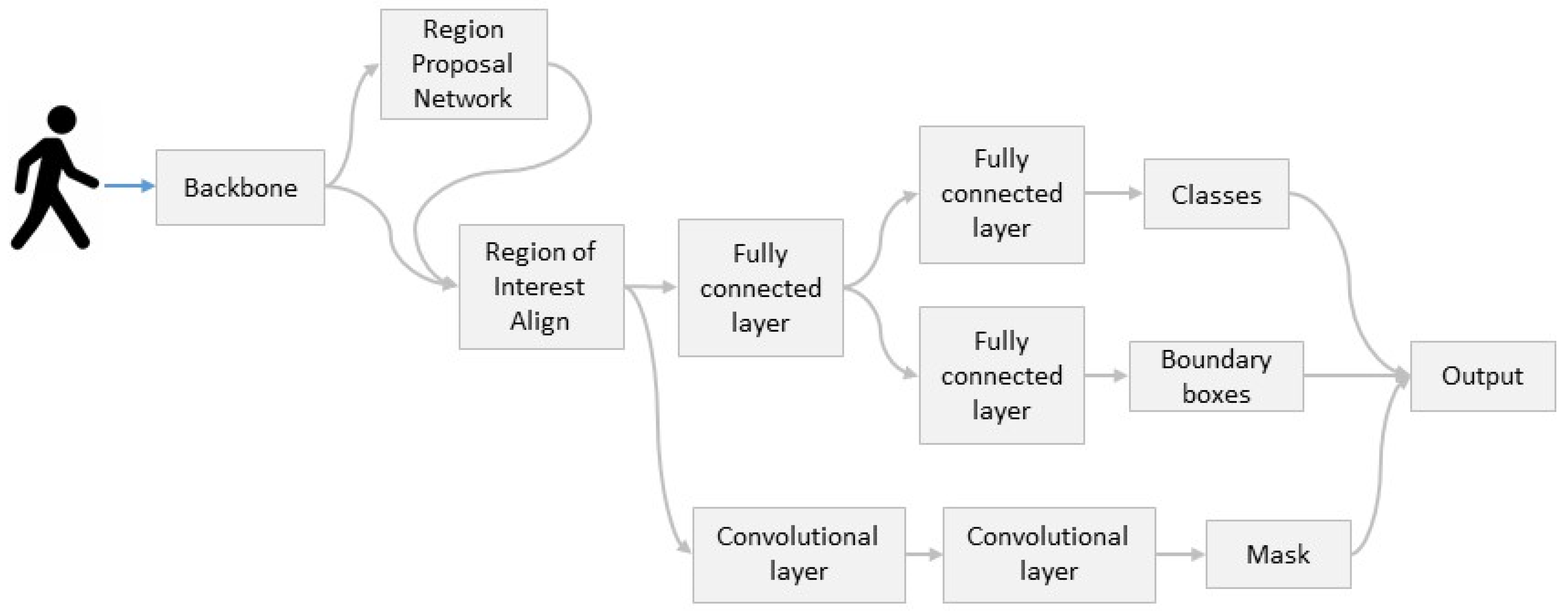
3. Mask R-CNN
4. Methodology
4.1. Transfer Learning and Fine Tuning
4.2. Backbones
4.2.1. Alex Net
4.2.2. Mobile Net V2
4.2.3. ResNet50
4.2.4. VGG11
4.2.5. VGG13
4.2.6. VGG16
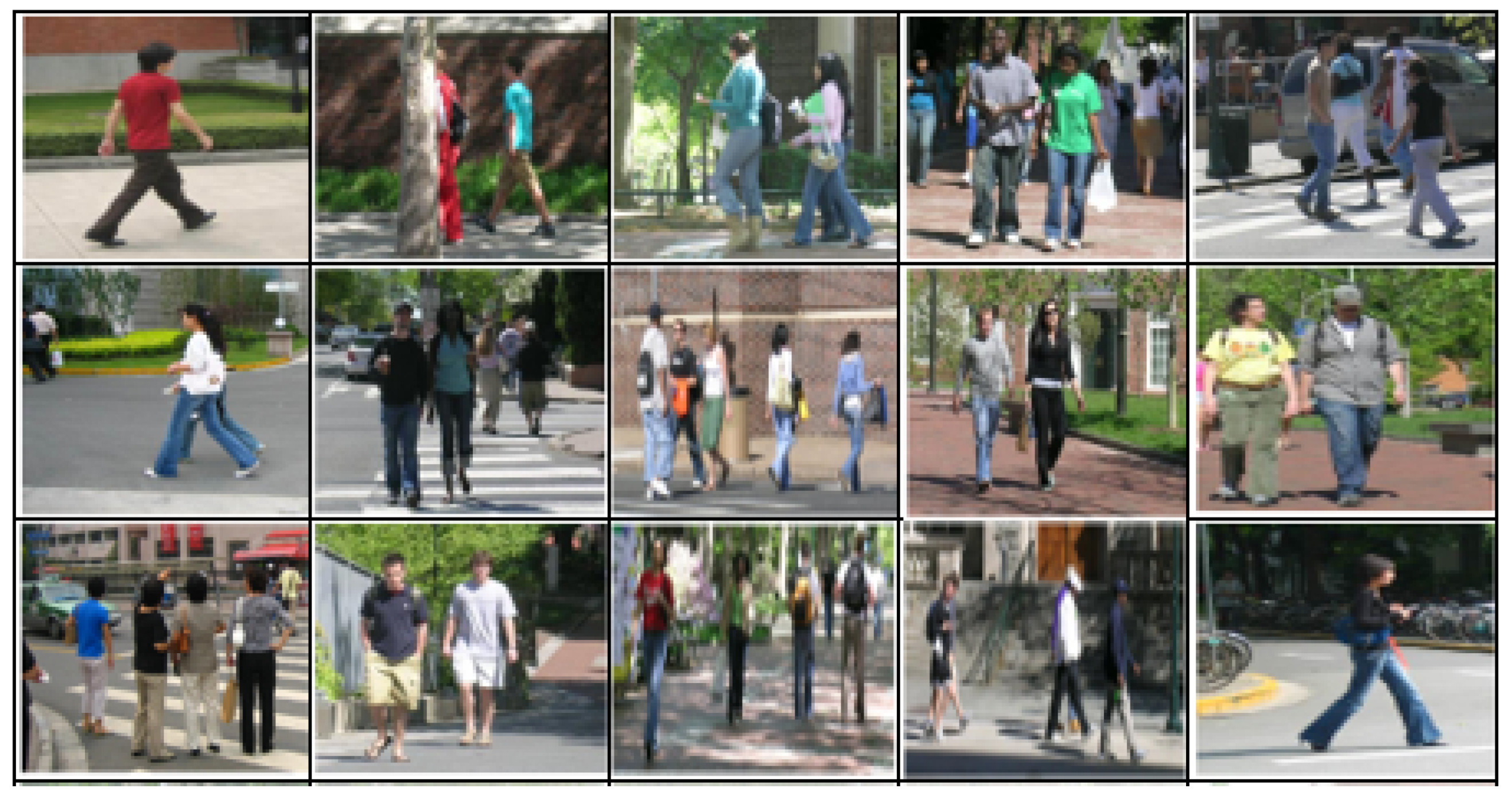
5. Dataset
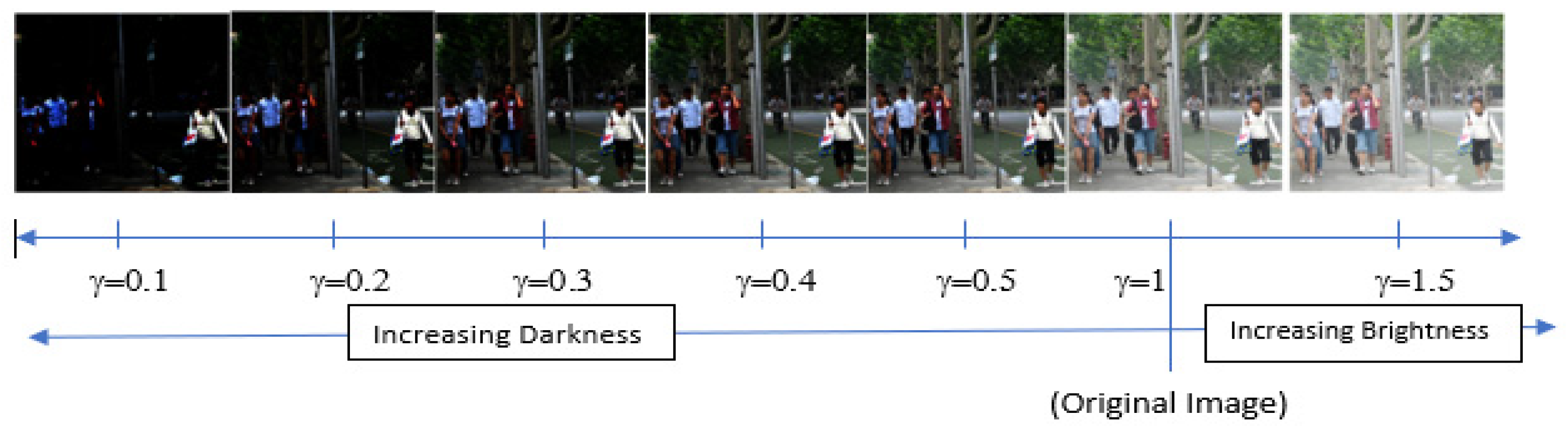
6. Inverse Gamma Correction
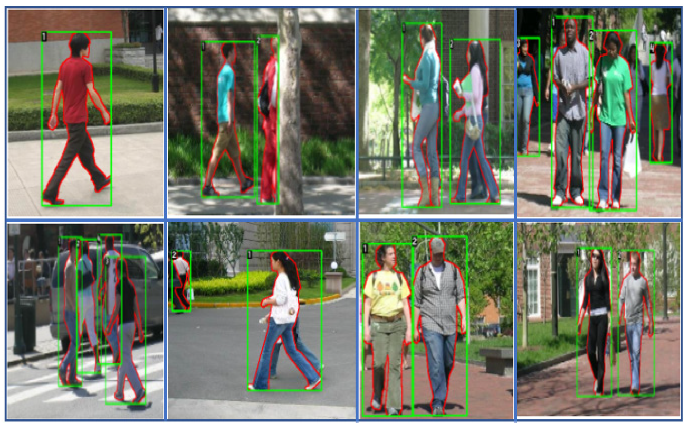
7. Instance Segmentation
8. Results
9. Evaluation

| Top Score Value | ||||||||
|---|---|---|---|---|---|---|---|---|
| Test Images | 0.1 | 0.2 | 0.3 | 0.4 | 0.5 | 1 | 1.5 | |
| 0 | 0.1092 | 0.0587 | 0 | 0.0648 | 0.1715 | 0.5374 | 0.1118 | |
| 1 | 0.0854 | 0 | 0 | 0.0685 | 0.158 | 0.5369 | 0.069 | |
| 2 | 0.1225 | 0.0594 | 0.0603 | 0.0698 | 0.1518 | 0.5276 | 0.0852 | |
| 3 | 0.1541 | 0.0917 | 0 | 0.0731 | 0.1479 | 0.5605 | 0.1314 | |
| 4 | 0.1415 | 0.0585 | 0.0639 | 0.0824 | 0.1341 | 0.5486 | 0.0953 | |
| 5 | 0.1737 | 0.121 | 0 | 0.0913 | 0.1385 | 0.5462 | 0.0887 | |
| 6 | 0.1359 | 0.08 | 0.0624 | 0.0841 | 0.1049 | 0.5342 | 0.1157 | |
| 7 | 0.1526 | 0.0743 | 0 | 0.0525 | 0.1144 | 0.5403 | 0.1174 | |
| 8 | 0.1327 | 0.0533 | 0.0509 | 0.0872 | 0.1341 | 0.5252 | 0.0732 | |
| 9 | 0.1198 | 0 | 0 | 0.0851 | 0.178 | 0.5135 | 0.1021 | |
| Average | 0.13274 | 0.05969 | 0.02375 | 0.07588 | 0.14332 | 0.53704 | 0.09898 | |
| Top Score Value | ||||||||
|---|---|---|---|---|---|---|---|---|
| Test Images | 0.1 | 0.2 | 0.3 | 0.4 | 0.5 | 1 | 1.5 | |
| 0 | 0.1037 | 0.0935 | 0.0874 | 0.0826 | 0.122 | 0.4899 | 0.1032 | |
| 1 | 0.1021 | 0 | 0 | 0 | 0.0781 | 0.6261 | 0.0756 | |
| 2 | 0.109 | 0.0975 | 0.0661 | 0.0771 | 0.1038 | 0.6609 | 0.1351 | |
| 3 | 0.114 | 0.0896 | 0.0813 | 0.077 | 0.1073 | 0.6643 | 0.1171 | |
| 4 | 0.1365 | 0.112 | 0.0945 | 0.0606 | 0.1363 | 0.6215 | 0.0946 | |
| 5 | 0.1389 | 0.1277 | 0.059 | 0.0858 | 0.1089 | 0.6422 | 0.0807 | |
| 6 | 0.0878 | 0.0907 | 0.0746 | 0.0616 | 0.0927 | 0.6987 | 0.0856 | |
| 7 | 0.0985 | 0.0954 | 0.0774 | 0.0676 | 0.1007 | 0.6773 | 0.1011 | |
| 8 | 0.1076 | 0.1087 | 0.0947 | 0.0699 | 0.127 | 0.6693 | 0.1194 | |
| 9 | 0.1045 | 0.0549 | 0.0725 | 0.071 | 0.0851 | 0.5985 | 0.0569 | |
| Average | 0.11026 | 0.087 | 0.07075 | 0.06532 | 0.10619 | 0.63487 | 0.09693 | |
| Top Score Value | ||||||||
|---|---|---|---|---|---|---|---|---|
| Test Images | 0.1 | 0.2 | 0.3 | 0.4 | 0.5 | 1 | 1.5 | |
| 0 | 0.677 | 0.8755 | 0.8625 | 0.8822 | 0.8686 | 0.9988 | 0.88 | |
| 1 | 0.6161 | 0.9058 | 0.9036 | 0.9032 | 0.9071 | 0.9976 | 0.92 | |
| 2 | 0.6315 | 0.8889 | 0.88 | 0.8846 | 0.8716 | 0.9958 | 0.895 | |
| 3 | 0.6486 | 0.8687 | 0.8721 | 0.8778 | 0.8729 | 0.9966 | 0.8862 | |
| 4 | 0.613 | 0.8566 | 0.8305 | 0.8427 | 0.8383 | 0.9967 | 0.8588 | |
| 5 | 0.6082 | 0.8319 | 0.8023 | 0.7977 | 0.7933 | 0.9904 | 0.8418 | |
| 6 | 0.6438 | 0.8465 | 0.8541 | 0.8556 | 0.856 | 0.9972 | 0.8872 | |
| 7 | 0.6061 | 0.8737 | 0.8579 | 0.8532 | 0.8507 | 0.9982 | 0.8841 | |
| 8 | 0.5955 | 0.8308 | 0.8229 | 0.8121 | 0.8116 | 0.998 | 0.8189 | |
| 9 | 0.5269 | 0.8534 | 0.8821 | 0.8685 | 0.866 | 0.9985 | 0.8851 | |
| Average | 0.61667 | 0.86318 | 0.8568 | 0.85776 | 0.85361 | 0.99678 | 0.87571 | |
| Top Score Value | ||||||||
|---|---|---|---|---|---|---|---|---|
| Test Images | 0.1 | 0.2 | 0.3 | 0.4 | 0.5 | 1 | 1.5 | |
| 0 | 0.1889 | 0.1629 | 0.1914 | 0.1337 | 0.1733 | 0.7792 | 0.175 | |
| 1 | 0.0851 | 0.0993 | 0.086 | 0.1407 | 0.1965 | 0.8253 | 0.1482 | |
| 2 | 0.2229 | 0.1983 | 0.2062 | 0.133 | 0.2092 | 0.7748 | 0.1773 | |
| 3 | 0.2128 | 0.2215 | 0.2034 | 0.1219 | 0.2051 | 0.7706 | 0.1749 | |
| 4 | 0.1816 | 0.1708 | 0.1674 | 0.1421 | 0.2152 | 0.75 | 0.1775 | |
| 5 | 0.2326 | 0.231 | 0.2264 | 0.1227 | 0.1889 | 0.7653 | 0.1853 | |
| 6 | 0.1875 | 0.2072 | 0.1849 | 0.1176 | 0.1843 | 0.819 | 0.1767 | |
| 7 | 0.2115 | 0.1955 | 0.1959 | 0.139 | 0.1741 | 0.7952 | 0.1643 | |
| 8 | 0.2199 | 0.1863 | 0.2001 | 0.1452 | 0.2207 | 0.7579 | 0.1791 | |
| 9 | 0.1191 | 0.1097 | 0.1057 | 0.1298 | 0.1668 | 0.5576 | 0.2018 | |
| Average | 0.18619 | 0.17825 | 0.17674 | 0.13257 | 0.19341 | 0.75949 | 0.17601 | |
| Top Score Value | ||||||||
|---|---|---|---|---|---|---|---|---|
| Test Images | 0.1 | 0.2 | 0.3 | 0.4 | 0.5 | 1 | 1.5 | |
| 0 | 0.0706 | 0.1952 | 0.1302 | 0.165 | 0.1275 | 0.7111 | 0.1958 | |
| 1 | 0.0685 | 0.08 | 0.1694 | 0.1439 | 0.1375 | 0.7227 | 0.1742 | |
| 2 | 0.0671 | 0.1873 | 0.1622 | 0.1585 | 0.1297 | 0.7334 | 0.2018 | |
| 3 | 0.064 | 0.1768 | 0.14 | 0.1602 | 0.1176 | 0.7446 | 0.2033 | |
| 4 | 0.0703 | 0.1739 | 0.1605 | 0.1666 | 0.1199 | 0.6729 | 0.2156 | |
| 5 | 0.0854 | 0.1767 | 0.1481 | 0.1617 | 0.1222 | 0.7071 | 0.193 | |
| 6 | 0.1682 | 0.1718 | 0.1436 | 0.1728 | 0.1383 | 0.7209 | 0.2092 | |
| 7 | 0.0644 | 0.1727 | 0.1269 | 0.1692 | 0.1232 | 0.7559 | 0.2012 | |
| 8 | 0.0714 | 0.18 | 0.1202 | 0.1314 | 0.1218 | 0.7607 | 0.2041 | |
| 9 | 0.0676 | 0.0995 | 0.1205 | 0.1205 | 0.1181 | 0.688 | 0.2397 | |
| Average | 0.07975 | 0.16139 | 0.14216 | 0.15498 | 0.12558 | 0.72173 | 0.20379 | |
| Top Score Value | ||||||||
|---|---|---|---|---|---|---|---|---|
| Test Images | 0.1 | 0.2 | 0.3 | 0.4 | 0.5 | 1 | 1.5 | |
| 0 | 0.0962 | 0.0939 | 0.0966 | 0.1385 | 0.0848 | 0.5924 | 0.1109 | |
| 1 | 0.0922 | 0.0702 | 0.0851 | 0.1592 | 0.114 | 0.588 | 0.109 | |
| 2 | 0.0976 | 0.0807 | 0.0973 | 0.1341 | 0.0857 | 0.5485 | 0.1101 | |
| 3 | 0.0923 | 0.0792 | 0.0923 | 0.1414 | 0.0779 | 0.5059 | 0.1163 | |
| 4 | 0.0936 | 0.0792 | 0.0958 | 0.16 | 0.1059 | 0.5174 | 0.114 | |
| 5 | 0.0986 | 0.1023 | 0.0995 | 0.1493 | 0.1453 | 0.5552 | 0.1186 | |
| 6 | 0.0891 | 0.1008 | 0.0953 | 0.1225 | 0.0978 | 0.5839 | 0.1133 | |
| 7 | 0.0988 | 0.0841 | 0.0939 | 0.145 | 0.0757 | 0.5848 | 0.1193 | |
| 8 | 0.0922 | 0.08 | 0.0998 | 0.1355 | 0.0792 | 0.5436 | 0.1232 | |
| 9 | 0.0903 | 0.0732 | 0.0885 | 0.1583 | 0.0941 | 0.5375 | 0.1146 | |
| Average | 0.09409 | 0.08436 | 0.09441 | 0.14438 | 0.09604 | 0.55572 | 0.11493 | |
10. Conclusions
Author Contributions
Funding
Institutional Review Board Statement
Informed Consent Statement
Data Availability Statement
Conflicts of Interest
References
- Borek, J.; Groelke, B.; Earnhardt, C.; Vermillion, C. Economic Optimal Control for Minimizing Fuel Consumption of Heavy-Duty Trucks in a Highway Environment. IEEE Trans. Control. Syst. Technol. 2019, 28, 1652–1664. [Google Scholar] [CrossRef]
- Torabi, S.; Bellone, M.; Wahde, M. Energy minimization for an electric bus using a genetic algorithm. Eur. Transp. Res. Rev. 2020, 12, 2. [Google Scholar] [CrossRef]
- Fényes, D.; Németh, B.; Gáspár, P. A Novel Data-Driven Modeling and Control Design Method for Autonomous Vehicles. Energies 2021, 14, 517. [Google Scholar] [CrossRef]
- Aymen, F.; Mahmoudi, C. A novel energy optimization approach for electrical vehicles in a smart city. Energies 2019, 12, 929. [Google Scholar] [CrossRef] [Green Version]
- Skrúcaný, T.; Kendra, M.; Stopka, O.; Milojević, S.; Figlus, T.; Csiszár, C. Impact of the electric mobility implementation on the greenhouse gases production in central European countries. Sustainability 2019, 11, 4948. [Google Scholar] [CrossRef] [Green Version]
- Csiszár, C.; Földes, D. System model for autonomous road freight transportation. Promet-Traffic Transp. 2018, 30, 93–103. [Google Scholar] [CrossRef] [Green Version]
- Lu, Q.; Tettamanti, T. Traffic Control Scheme for Social Optimum Traffic Assignment with Dynamic Route Pricing for Automated Vehicles. Period. Poly. Transp. Eng. 2021, 49, 301–307. [Google Scholar] [CrossRef]
- Li, Q.; He, T.; Fu, G. Judgment and optimization of video image recognition in obstacle detection in intelligent vehicle. Mech. Syst. Signal Process. 2020, 136, 106406. [Google Scholar] [CrossRef]
- Yang, L.; Liu, Z.; Wang, X.; Yu, X.; Wang, G.; Shen, L. Image-Based Visual Servo Tracking Control of a Ground Moving Target for a Fixed-Wing Unmanned Aerial Vehicle. J. Intell. Robot. Syst. 2021, 102, 81. [Google Scholar] [CrossRef]
- Junaid, A.B.; Konoiko, A.; Zweiri, Y.; Sahinkaya, M.N.; Seneviratne, L. Autonomous wireless self-charging for multi-rotor unmanned aerial vehicles. Energies 2017, 10, 803. [Google Scholar] [CrossRef]
- Lee, S.H.; Kim, B.J.; Lee, S.B. Study on Image Correction and Optimization of Mounting Positions of Dual Cameras for Vehicle Test. Energies 2021, 14, 4857. [Google Scholar] [CrossRef]
- Tschürtz, H.; Gerstinger, A. The Safety Dilemmas of Autonomous Driving. In Proceedings of the 2021 Zooming Innovation in Consumer Technologies Conference (ZINC), Novi Sad, Serbia, 26–27 May 2021; pp. 54–58. [Google Scholar]
- Zhao, Z.Q.; Zheng, P.; Xu, S.T.; Wu, X. Object Detection with Deep Learning: A Review. IEEE Trans. Neural Netw. Learn. Syst. 2019, 30, 3212–3232. [Google Scholar] [CrossRef] [PubMed] [Green Version]
- Kohli, P.; Chadha, A. Enabling pedestrian safety using computer vision techniques: A case study of the 2018 uber inc. self-driving car crash. Lect. Notes Netw. Syst. 2020, 69, 261–279. [Google Scholar] [CrossRef] [Green Version]
- Barba-Guaman, L.; Naranjo, J.E.; Ortiz, A. Deep learning framework for vehicle and pedestrian detection in rural roads on an embedded GPU. Electron 2020, 9, 589. [Google Scholar] [CrossRef] [Green Version]
- Simhambhatla, R.; Okiah, K.; Slater, R. Self-Driving Cars: Evaluation of Deep Learning Techniques for Object Detection in Different Driving Conditions. SMU Data Sci. Rev. 2019, 2, 23. [Google Scholar]
- Cao, C.; Wang, B.; Zhang, W.; Zeng, X.; Yan, X.; Feng, Z.; Liu, Y.; Wu, Z. An Improved Faster R-CNN for Small Object Detection. IEEE Access 2019, 7, 106838–106846. [Google Scholar] [CrossRef]
- Sandler, M.; Howard, A.; Zhu, M.; Zhmoginov, A.; Chen, L.C. MobileNetV2: Inverted Residuals and Linear Bottlenecks. In Proceedings of the IEEE Conference on Computer Vision and Pattern Recognition (CVPR), Salt Lake City, UT, USA, 18–23 June 2018; pp. 4510–4520. [Google Scholar] [CrossRef] [Green Version]
- Alganci, U.; Soydas, M.; Sertel, E. Comparative research on deep learning approaches for airplane detection from very high-resolution satellite images. Remote Sens. 2020, 12, 458. [Google Scholar] [CrossRef] [Green Version]
- Huang, R.; Pedoeem, J.; Chen, C. YOLO-LITE: A Real-Time Object Detection Algorithm Optimized for Non-GPU Computers. In Proceedings of the 2018 IEEE International Conference on Big Data, Seattle, WA, USA, 10–13 December 2018; pp. 2503–2510. [Google Scholar] [CrossRef] [Green Version]
- Redmon, J.; Farhadi, A. YOLO v.3. Tech Rep. 2018, pp. 1–6. Available online: https://pjreddie.com/media/files/papers/YOLOv3.pdf (accessed on 1 February 2021).
- Suhail, A.; Jayabalan, M.; Thiruchelvam, V. Convolutional neural network based object detection: A review. J. Crit. Rev. 2020, 7, 786–792. [Google Scholar] [CrossRef]
- Lokanath, M.; Kumar, K.S.; Keerthi, E.S. Accurate object classification and detection by faster-R-CNN. IOP Conf. Ser. Mater. Sci. Eng. 2017, 263, 052028. [Google Scholar] [CrossRef]
- Girshick, R. Fast R-CNN. In Proceedings of the 2015 International Conference on Computer Vision (ICCV), Santiago, Chile, 7–13 December 2015; pp. 1440–1448. [Google Scholar] [CrossRef]
- Almubarak, H.; Bazi, Y.; Alajlan, N. Two-stage mask-R-CNN approach for detecting and segmenting the optic nerve head, optic disc, and optic cup in fundus images. Appl. Sci. 2020, 10, 3833. [Google Scholar] [CrossRef]
- Mahmoud, A.S.; Mohamed, S.A.; El-Khoribi, R.A.; AbdelSalam, H.M. Object detection using adaptive mask R-CNN in optical remote sensing images. Int. J. Intell. Eng. Syst. 2020, 13, 65–76. [Google Scholar] [CrossRef]
- Rezvy, S.; Zebin, T.; Braden, B.; Pang, W.; Taylor, S.; Gao, X.W. Transfer learning for endoscopy disease detection and segmentation with Mask-RCNN benchmark architecture. In Proceedings of the 2nd International Workshop and Challenge on Computer Vision in Endoscopy, Iowa City, IA, USA, 3 April 2020; pp. 68–72. [Google Scholar]
- Wu, X.; Wen, S.; Xie, Y.A. Improvement of Mask-R-CNN Object Segmentation Algorithm; Springer International Publishing: New York, NY, USA, 2019; Volume 11740. [Google Scholar]
- Penn-Fudan Database for Pedestrian Detection and Segmentation. Available online: https://www.cis.upenn.edu/~jshi/ped_html/index.html (accessed on 1 February 2021).
- Tv, C.R.T.; Crt, T.; Intensity, L.; Voltage, C.; Lcd, T. How to Match the Color Brightness of Automotive TFT-LCD Panels. pp. 1–6. Available online: https://www.renesas.com/us/en/document/whp/how-match-color-brightness-automotive-tft-lcd-panels (accessed on 1 February 2021).
- Farid, H. Blind inverse gamma correction. IEEE Trans. Image Process. 2001, 10, 1428–1433. [Google Scholar] [CrossRef] [PubMed]
- DeArman, A. The Wild, Wild West: A Case Study of Self-Driving Vehicle Testing in Arizona. 2010. Available online: https://arizonalawreview.org/the-wild-wild-west-a-case-study-of-self-driving-vehicle-testing-in-arizona/ (accessed on 1 February 2021).
- Mikusova, M. Crash avoidance systems and collision safety devices for vehicle. In Proceedings of the MATEC Web of Conferences: Dynamics of Civil Engineering and Transport Structures and Wind Engineering—DYN-WIND’2017, Trstená, Slovak Republic, 21–25 May 2017; Volume 107, p. 00024. [Google Scholar]
- Ammirato, P.; Berg, A.C. A Mask-R-CNN Baseline for Probabilistic Object Detection. 2019. Available online: http://arxiv.org/abs/1908.03621 (accessed on 1 February 2021).
- Zhang, Y.; Chu, J.; Leng, L.; Miao, J. Mask-refined R-CNN: A network for refining object details in instance segmentation. Sensors 2020, 20, 1010. [Google Scholar] [CrossRef] [Green Version]
- Michele, A.; Colin, V.; Santika, D.D. Mobilenet convolutional neural networks and support vector machines for palmprint recognition. Procedia Comput. Sci. 2019, 157, 110–117. [Google Scholar] [CrossRef]
- Sharma, V.; Mir, R.N. Saliency guided faster-R-CNN (SGFr-R-CNN) model for object detection and recognition. J. King Saud. Univ.-Comput. Inf. Sci. 2019. [Google Scholar] [CrossRef]
- Ren, S.; He, K.; Girshick, R.; Sun, J. Faster R-CNN: Towards Real-Time Object Detection with Region Proposal Networks. IEEE Trans. Pattern Anal. Mach. Intell. 2017, 39, 1137–1149. [Google Scholar] [CrossRef] [Green Version]
- Girshick, R.; Donahue, J.; Darrell, T.; Malik, J. Region-Based Convolutional Networks for Accurate Object Detection and Segmentation. IEEE Trans. Pattern Anal. Mach. Intell. 2016, 38, 142–158. [Google Scholar] [CrossRef] [PubMed]
- Özgenel, F.; Sorguç, A.G. Performance comparison of pretrained convolutional neural networks on crack detection in buildings. In Proceedings of the 35th International Symposium on Automation and Robotics in Construction (ISARC 2018), Berlin, Germany, 20–25 July 2018. [Google Scholar] [CrossRef]
- Iglovikov, V.; Seferbekov, S.; Buslaev, A.; Shvets, A. TernausNetV2: Fully convolutional network for instance segmentation. In Proceedings of the IEEE Conference on Computer Vision and Pattern Recognition (CVPR) Workshops, Salt Lake City, UT, USA, 18–23 June 2018; pp. 228–232. [Google Scholar] [CrossRef] [Green Version]
- Saha, R. Transfer Learning—A Comparative Analysis. December 2018. Available online: https://www.researchgate.net/publication/329786975_Transfer_Learning_-_A_Comparative_Analysis?channel=doi&linkId=5c1a9767299bf12be38bb098&showFulltext=true (accessed on 1 February 2021).
- Girshick, R.; Donahue, J.; Darrell, T.; Malik, J.; Berkeley, U.C.; Malik, J. Rich feature hierarchies for accurate object detection and semantic segmentation. In Proceedings of the IEEE Conference on Computer Vision and Pattern Recognition, Columbus, OH, USA, 23–28 June 2014; Volume 1, p. 5000. [Google Scholar] [CrossRef] [Green Version]
- Zhao, Y.; Han, R.; Rao, Y. A new feature pyramid network for object detection. In Proceedings of the 2019 International Conference on Virtual Reality and Intelligent Systems (ICVRIS), Jishou, China, 14–15 September 2019; pp. 428–431. [Google Scholar] [CrossRef]
- Krizhevsky, A.; Sutskever, I.; Hinton, G.E. ImageNet Classification with Deep Convolutional Neural Networks. Commun. ACM 2017, 60, 84–90. [Google Scholar] [CrossRef]
- Martin, C.H.; Mahoney, M.W. Traditional and heavy tailed self regularization in neural network models. In Proceedings of the 36th International Conference on Machine Learning, Long Beach, CA, USA, 9–15 June 2019; pp. 7563–7572. [Google Scholar]
- Alom, M.Z.; Taha, T.M.; Yakopcic, C.; Westberg, S.; Sidike, P.; Nasrin, M.S.; Van Esesn, B.C.; Awwal, A.A.S.; Asari, V.K. The History Began from AlexNet: A Comprehensive Survey on Deep Learning Approaches. 2018. Available online: http://arxiv.org/abs/1803.01164 (accessed on 1 February 2021).
- Almisreb, A.A.; Jamil, N.; Din, N.M. Utilizing AlexNet Deep Transfer Learning for Ear Recognition. In Proceedings of the 2018 Fourth International Conference on Information Retrieval and Knowledge Management (CAMP), Kota Kinabalu, Malaysia, 26–28 March 2018; pp. 8–12. [Google Scholar] [CrossRef]
- Sudha, K.K.; Sujatha, P. A qualitative analysis of googlenet and alexnet for fabric defect detection. Int. J. Recent Technol. Eng. 2019, 8, 86–92. [Google Scholar]
- Howard, A.G.; Zhu, M.; Chen, B.; Kalenichenko, D.; Wang, W.; Weyand, T.; Andreetto, M.; Adam, H. MobileNets: Efficient Convolutional Neural Networks for Mobile Vision Applications. 2017. Available online: http://arxiv.org/abs/1704.04861 (accessed on 1 February 2021).
- Reddy, A.S.B.; Juliet, D.S. Transfer learning with RESNET-50 for malaria cell-image classification. In Proceedings of the 2019 International Conference on Communication and Signal Processing (ICCSP), Chennai, India, 4–6 April 2019; pp. 945–949. [Google Scholar] [CrossRef]
- Rezende, E.; Ruppert, G.; Carvalho, T.; Ramos, F.; de Geus, P. Malicious software classification using transfer learning of ResNet-50 deep neural network. In Proceedings of the 2017 16th IEEE International Conference on Machine Learning and Applications (ICMLA), Cancun, Mexico, 18–21 December 2017; pp. 1011–1014. [Google Scholar] [CrossRef]
- Mikami, H.; Suganuma, H.; U-chupala, P.; Tanaka, Y.; Kageyama, Y. ImageNet/ResNet-50 Training in 224 Seconds, No. Table 2. 2018. Available online: http://arxiv.org/abs/1811.05233 (accessed on 1 February 2021).
- Simonyan, K.; Zisserman, A. Very deep convolutional networks for large-scale image recognition. In Proceedings of the 2014 International Conference on Learning Representations, Banff, AB, Canada, 14–16 April 2014; pp. 1–14. [Google Scholar]
- Rostianingsih, S.; Setiawan, A.; Halim, C.I. COCO (Creating Common Object in Context) Dataset for Chemistry Apparatus. Procedia Comput. Sci. 2020, 171, 2445–2452. [Google Scholar] [CrossRef]
- Lin, T.Y.; Maire, M.; Belongie, S.; Hays, J.; Perona, P.; Ramanan, D.; Dollár, P.; Zitnick, C.L. Microsoft COCO: Common Objects in Context. In Computer Vision—ECCV 2014; Fleet, D., Pajdla, T., Schiele, B., Tuytelaars, T., Eds.; Springer: Cham, Switzerland, 2017; Volume 8693, pp. 740–755. [Google Scholar] [CrossRef] [Green Version]
- Everingham, M.; van Gool, L.; Williams, C.K.I.; Winn, J.; Zisserman, A. The pascal visual object classes (VOC) challenge. Int. J. Comput. Vis. 2010, 88, 303–338. [Google Scholar] [CrossRef] [Green Version]
- Python Deep Learning Cookbook. Available online: https://livrosdeamor.com.br/documents/python-deep-learning-cookbook-indra-den-bakker-5c8c74d0a1136 (accessed on 1 February 2021).
- Guan, Q.; Wang, Y.; Ping, B.; Li, D.; Du, J.; Qin, Y.; Lu, H.; Wan, X.; Xiang, J. Deep convolutional neural network VGG-16 model for differential diagnosing of papillary thyroid carcinomas in cytological images: A pilot study. J. Cancer 2019, 10, 4876–4882. [Google Scholar] [CrossRef] [PubMed]
- Tammina, S. Transfer learning using VGG-16 with Deep Convolutional Neural Network for Classifying Images. Int. J. Sci. Res. Publ. 2019, 9, 9420. [Google Scholar] [CrossRef]
- Veit, A.; Matera, T.; Neumann, L.; Matas, J.; Belongie, S. COCO-Text: Dataset and Benchmark for Text Detection and Recognition in Natural Images. September 2016. Available online: http://arxiv.org/abs/1601.07140 (accessed on 1 February 2021).
- Mahamdioua, M.; Benmohammed, M. New Mean-Variance Gamma Method for Automatic Gamma Correction. Int. J. Image Graph. Signal Process. 2017, 9, 41–54. [Google Scholar] [CrossRef] [Green Version]
- Jin, L.; Chen, Z.; Tu, Z. Object Detection Free Instance Segmentation with Labeling Transformations. 2016, p. 1. Available online: http://arxiv.org/abs/1611.08991 (accessed on 1 February 2021).
| VGG Variant | VGG11 | VGG13 | VGG16 |
|---|---|---|---|
| Error Rate | 10.4% | 9.9% | 9.4% |
| (a) | ||
|---|---|---|
| Normalize | Mean | Standard Deviation |
| 0.485 | 0.229 | |
| 0.456 | 0.224 | |
| 0.406 | 0.225 | |
| (b) | ||
| Resize | Minimum Size | Maximum Size |
| 800 | 1333 | |
| Backbone | λc | λb | λm | λ0 | λr | λT |
|---|---|---|---|---|---|---|
| Alex Net | 0.0569 | 0.1345 | 0.3612 | 0.1672 | 1.8658 | 2.5856 |
| Mobile Net V2 | 0.0603 | 0.1248 | 0.4285 | 0.17 | 1.5136 | 2.2972 |
| ResNet50 | 0.0199 * | 0.0279 * | 0.1115 * | 0.0002 * | 0.0022 * | 0.1617 * |
| VGG11 | 0.2872 | 0.4664 | 0.2734 | 0.2229 | 2.5641 | 3.814 |
| VGG13 | 0.3089 | 0.4694 | 0.2839 | 0.2462 | 2.6469 | 3.9553 |
| VGG16 | 0.4191 | 0.6803 | 0.3671 | 0.2607 | 2.8196 | 4.5468 |
| Backbone | AP (Bbox) | AR (Bbox) | AP (Segm) | AR (Segm) |
|---|---|---|---|---|
| Alex Net | 0.213 | 0.409 | 0.173 | 0.357 |
| Mobile Net V2 | 0.175 | 0.38 | 0.105 | 0.23 |
| Resnet50 | 0.844 * | 0.883 * | 0.774 * | 0.813 * |
| VGG11 | 0.233 | 0.413 | 0.298 | 0.427 |
| VGG13 | 0.237 | 0.42 | 0.2878 | 0.416 |
| VGG16 | 0.148 | 0.359 | 0.188 | 0.339 |
| Backbone | Model Time | Evaluator Time |
|---|---|---|
| Alex Net | 0.0452 | 0.0165 |
| Mobile Net V2 | 0.0606 | 0.0111 |
| ResNet50 | 0.075 | 0.003 * |
| VGG11 | 0.046 * | 0.0094 |
| VGG13 | 0.0699 | 0.0069 |
| VGG16 | 0.0827 | 0.0115 |
| γ = 0.1 | γ = 0.2 | γ = 0.3 | γ = 0.4 | γ = 0.5 | γ = 1 | γ = 1.5 | |
|---|---|---|---|---|---|---|---|
| Mask R-CNN_AlexNet | 0.13274 | 0.05969 | 0.02375 | 0.07588 | 0.14332 | 0.53704 | 0.09898 |
| Mask R-CNN_MobileNet | 0.11026 | 0.087 | 0.07075 | 0.06532 | 0.10619 | 0.63487 | 0.09693 |
| Mask R-CNN_ResNet50 | 0.61667 | 0.86318 | 0.8568 | 0.85776 | 0.85361 | 0.99678 | 0.87571 |
| Mask R-CNN_VGG11 | 0.18619 | 0.17825 | 0.17674 | 0.13257 | 0.19341 | 0.75949 | 0.17601 |
| Mask R-CNN_VGG13 | 0.07975 | 0.16139 | 0.14216 | 0.15498 | 0.12558 | 0.72173 | 0.20379 |
| Mask R-CNN_VGG16 | 0.09409 | 0.08436 | 0.09441 | 0.14438 | 0.09604 | 0.55572 | 0.11493 |
Publisher’s Note: MDPI stays neutral with regard to jurisdictional claims in published maps and institutional affiliations. |
© 2021 by the authors. Licensee MDPI, Basel, Switzerland. This article is an open access article distributed under the terms and conditions of the Creative Commons Attribution (CC BY) license (https://creativecommons.org/licenses/by/4.0/).
Share and Cite
Junaid, M.; Szalay, Z.; Török, Á. Evaluation of Non-Classical Decision-Making Methods in Self Driving Cars: Pedestrian Detection Testing on Cluster of Images with Different Luminance Conditions. Energies 2021, 14, 7172. https://doi.org/10.3390/en14217172
Junaid M, Szalay Z, Török Á. Evaluation of Non-Classical Decision-Making Methods in Self Driving Cars: Pedestrian Detection Testing on Cluster of Images with Different Luminance Conditions. Energies. 2021; 14(21):7172. https://doi.org/10.3390/en14217172
Chicago/Turabian StyleJunaid, Mohammad, Zsolt Szalay, and Árpád Török. 2021. "Evaluation of Non-Classical Decision-Making Methods in Self Driving Cars: Pedestrian Detection Testing on Cluster of Images with Different Luminance Conditions" Energies 14, no. 21: 7172. https://doi.org/10.3390/en14217172
APA StyleJunaid, M., Szalay, Z., & Török, Á. (2021). Evaluation of Non-Classical Decision-Making Methods in Self Driving Cars: Pedestrian Detection Testing on Cluster of Images with Different Luminance Conditions. Energies, 14(21), 7172. https://doi.org/10.3390/en14217172