Abstract
Accurate prediction of the throttle value and state for wheel loaders can help to achieve autonomous operation, thereby reducing the cost and accident rate. However, existing methods based on a physical model cannot accurately reflect the operator’s driving habits and the interaction between wheel loaders and the environment. In this paper, a deep-learning-based prediction model is developed to predict the throttle value and state for wheel loaders by learning from driving data. Multiple long–short-term memory (LSTM) networks are used to extract the temporal features of different stages during the operation of the wheel loader. Two backward-propagation neural networks (BPNNs), which use the temporal feature extracted by LSTM as the input, are designed to output the final prediction results of throttle value and state, respectively. The proposed prediction model is trained and tested using the data from two different conditions. The end-to-end LSTM prediction model and BPNNs are used as benchmark models. The results indicate that the proposed prediction model has good prediction accuracy and adaptability. Furthermore, the relationship between the prediction performance and signal sampling frequency is also studied. The proposed prediction method that combines driving data and deep learning can make the throttle action conform to the decisions of an experienced operator, providing technical support for the autonomous operation of construction machinery.
1. Introduction
As the most common mobile construction machinery, wheel loaders are widely used in the construction and mining industry, which are the important economic sectors across the world [1], due to their flexibility and adaptability. The main task of wheel loaders is to transport materials, including soil and rock, from a site to nearby dumpsite or trucks in a complex and changing working environment [2]. Control of the throttle is critical to the operation of wheel loaders. Accurately predicting the throttle action of a wheel loader expert operator can better achieve autonomous operation. The predicted throttle action can be used to directly the machine to imitate the expert operator’s operations, to help achieve autonomous operation. In addition, predictions on the state of wheel loaders can be applied to model predictive control and energy management to achieve a good performance in terms of efficiency and fuel consumption.
The automation of construction machinery can reduce the cost and improve the safety of construction sites. Based on this, the last three decades have seen a growing trend towards the automation of construction machinery [3,4,5]. Many researchers have discussed the division method from manual operation to fully autonomous operation [6,7]. Dadhich et al. [8] proposed five steps to achieve the full automation of wheel loaders: manual operation, in-sight tele-operation, tele-remote operation, assisted tele-remote operation, fully autonomous. Despite the extensive research on automating construction machinery [9,10,11], a commercial system with autonomous construction machinery is still being explored [12]. Remote-operated construction machinery is being tried for commercial purposes [13,14]. However, this has led to a greater reduction in productivity and fuel efficiency [15] than manual operation because there are not enough sensory inputs to the remote operators. Therefore, to increase the fuel efficiency and productivity of construction machinery, it is necessary to improve the degree of automation of the loader to reduce the operator’s remote intervention.
Most previous works related to the automation of construction machinery are based on a physical model that requires accurate mathematical representations [16,17,18]. Meng et al. [10] presented a way of optimizing the bucket trajectory for the autonomous loading of load-haul-dump (LHD) machines by solving the optimal trajectory through optimizing the minimum energy consumption calculated by Coulomb’s passive earth pressure theory. Filla et al. [11] analyzed different autonomous scooping trajectories for wheel loaders by developing a simulation model of the uniform gravel pile. Shen and Frank [12,14] introduced dynamic programming into the solvution of the optimal control variable trajectory based on a mathematical model of the machine. However, these physical-model-based approaches have some common limitations. The method requires a dynamic model of construction machinery to be built, but the dynamic model simplifies machinery in the real world, and the dynamic model of machinery may change under the condition of wear during the operation. Additionally, modeling the interaction force between the tool and material is challenging, as the working environment is unpredictable and variable, and the properties of the different media to be excavated or moved are diverse.
The data-driven approach makes it possible to deal with the complex machinery dynamics [19,20,21,22] et al. used the data collected from tests to construct a nonlinear, non-parametric statistical model to predict the behavior of soil excavated by an excavator bucket. Heteroscedastic Gaussian process regression is used as the prediction framework. Machine learning, as a significant means of analyzing complicated data, can adjust its weight parameters by learning from data. In recent years, machine learning has made remarkable progress in solving pattern classification or prediction problems, such as image recognition [23], pattern recognition [24,25], and fault diagnosis [26]. Deep learning has been widely used in construction machinery [12,27,28]. Kim et al. [29] proposed a vision-based action recognition framework that considers the sequential working patterns of earthmoving machinery to recognize the operation types. The earthmoving machinery’s sequential patterns are modeled and trained with convolutional neural networks and double-layer long–short-term memory (LSTM).
Due to its powerful ability to characterize complicated systems, process big data, and automatically extract features, deep learning has feasibility and superiority in the prediction task. The deep-learning-based prediction has received great attention for the automated operation of machinery. Yao et al. [30] designed a two-stage Convolutional Neural Networks model, including a classifier and some regressors, to automatically extract image features to obtain the piled-up status and payload distribution of the current state. The final prediction result is output via a backward-propagation neural network. Luo et al. [31] proposed a framework to predict the pose of construction machinery based on historical motions and activity attributes. The Gated Recurrent Unit is used to predict future machine poses, considering working patterns and interaction characteristics. Shi et al. [32] constructed a deep long–short-term memory network to predict the brake pedal aperture for different braking types by combining the driving data of experienced drivers in different driving environments with deep learning. Xing et al. [33] proposed an energy-aware personalized joint time-series modeling approach based on a recurrent neural network and LSTM to accurately predict the trajectory and velocity of the vehicle. Dai et al. [34] employed two groups of LSTM networks to predict the trajectory of the target vehicle. One LSTM is used to model the target vehicle and the individual trajectory of the surrounding vehicle, and the other is used to model the interaction between the target vehicle and each of the surrounding vehicles.
In this study, based on driving data of the experienced operator, a deep-learning-based method is proposed to accurately predict the throttle value and states (including lift cylinder, tilt cylinder, engine speed, vehicle velocity) of wheel loaders to help achieve autonomous operation and make predictive control algorithms and energy management strategies work with an acceptable performance. The sensor signals of wheel loaders under different working conditions are used instead of images as an important basis for predicting the throttle value and states of wheel loaders, as images will be inevitably affected by occlusions, deviations in viewpoint and scale, ambient illumination, and other factors [35,36]. Considering the time series characteristics of the working process of wheel loaders, LSTM networks are used to extract features. To reduce the computation load, the prediction of throttle value and state share the same LSTM network structures and weights. Two backward-propagation neural networks (BPNNs) are introduced to output the prediction results, as the throttle is controlled by the driver and the state of the wheel loaders is randomly influenced by the environment. Each working cycle of wheel loaders consists of several working phases, which possess their own unique characteristics, so the prediction results at different stages are output by neural networks with different weights to improve the prediction accuracy. Two different materials are used to study the adaptability of the prediction model. The relationship between the prediction performance and signal sampling frequency is also studied. Compared with the existing works, the method proposed in this study does not require a physical model and can be applied to different working conditions. The method proposed in this study can provide technical support for the autonomous operation of construction machinery and contribute to the intelligent process of the mining and construction industry.
2. Background
2.1. Problem Statement
The task of wheel loaders is to remove materials, including soil and rock, from a material pile to a nearby dumpsite or an adjacent load receiver in the sophisticated and changing working environment. There are many operation modes for wheel-loaders, including I, V, and T-shaped modes, depending on the route taken by wheel loaders during the loading operation. The difference in operation modes increases the difficulty of data analysis. For wheel-loaders, the V-cycle, which is the most common work cycle, is adopted in this experiment, as illustrated in Figure 1. The single V-cycle is divided into six phases, namely, V1 forward with no load (start and approach the pile), V2 bucket filling (penetrates the pile and load), V3 backward with a full load (retract from the pile), V4 forward and hoisting (approach the dumper), V5 dumping, V6 backward with no load (retract from the dumper), as shown in Table 1.
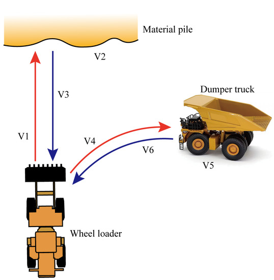
Figure 1.
V-cycle of wheel loaders.

Table 1.
V-cycle grouping.
During the entire working cycle of wheel loaders, the operator needs to constantly modulate the throttle to control the movement of the wheel loaders. The throttle greatly determines the productivity and fuel efficiency during the operation of wheel loaders. When the throttle value is too high, wheel slipping will occur, resulting in a loss of traction as the driving force exceeds the adhesion. Wheel slipping damages tires and results in significant increases in operational cost. While the throttle value is too small, the speed of the vehicle will be lower, resulting in a loss of productivity. For the V-cycle of wheel loaders, the road adhesion coefficient is different for different phases. The quality of the vehicle will vary widely due to loading and dumping, which impacts the throttle value. Therefore, in the process of driving, experienced operators are required to perceive the environment information and select the appropriate throttle value. In this paper, the throttle value of the next moment is predicted.
Lift cylinder pressure, tilt cylinder pressure, engine speed and vehicle velocity are all crucial for wheel loaders. Lift cylinder pressure and tilt cylinder pressure can help to identify the working-cycle stages of wheel loaders. Engine speed and vehicle velocity play an important role in energy management. In this paper, the four parameters are called the state of wheel loaders, and every parameter has a corresponding prediction value. The state prediction is the basis of many control technologies, including model predictive control. The state of wheel loaders is affected by the operator’s driving action and the environment, so the state prediction cannot only take their internal dynamics into account. In the operation process, in addition to the current state, operators usually need to consider the past actions and state of wheel loaders. Thus, the throttle value and state prediction of wheel loaders needs to consider the time series characteristics of the working process.
2.2. LSTM Network
Deep learning models automatically learn multiple levels of representations and abstractions from the data [37], which solves the problem that features need to be manually designed in traditional machine learning. Recurrent neural network (RNN) is a type of neural network specialized for the processing of sequence data. However, in practice, a simple RNN cannot cope with the challenge of long-term dependence.
The most efficient sequence model used in practical applications is called gated RNN, which is based on the idea of creating paths through time that have derivatives that neither vanish nor explode. Long short-term memory (LSTM) [38] is a type of gated RNN and a popular solution for processing sequence data. It has been shown to learn long-term dependencies more easily than simple recurrent architectures through gating units. Compared to the gated recurrent unit (GRU), a simpler gated RNN, LSTM is more powerful and more flexible, since it has three gates instead of two. Thus, LSTM is applied in this paper.
The LSTM block diagram is illustrated in Figure 2. The most crucial component of LSTM is the cell state, which is the horizontal line running through the top of the figure, making it easy for information to flow without changing. LSTM’s ability to remove or add information to the cell state is controlled by the structure called gates. Gates consisting of a sigmoid neural net layer and a pointwise multiplication operation can selectively let information through. The first step of LSTM is to determine which information is discarded from the cell state. This decision is made by the forget gate, which outputs a number between 0 and 1 for each number in the previous cell state. Second, the new information that will be stored in the cell state needs to be determined. The input gate determines which values will be updated and a tanh layer creates a vector of new candidate values that could be used to update the current cell state. Finally, the current cell state and output gate are used to output the hidden state. The process of LSTM can be expressed as follows:
where , and represent the hidden states, cell state and the input sequence of LSTM at time t, respectively. , and represent input gate, forget gate and output gate, respectively. W and b represent the weights and bias , respectively. and represent cell state at time t and candidate cell state at time t. ∗ is the element-wise product.
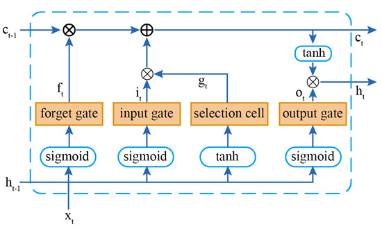
Figure 2.
Illustration of Long short-term memory (LSTM).
3. Methodology
3.1. The Overview of the Proposed Deep Learning-Based Framwork
Operators of different proficiency levels can account for great differences in productivity and fuel efficiency. Consequently, deep learning is used to predict the throttle value of wheel loaders based on the driving data of experienced operators so that the driving process of wheel loaders conforms to the driving decisions of experienced operators to meet the vehicle’s operational requirements, even in sophisticated driving environments, while ensuring productivity and fuel efficiency. Meanwhile, based on the temporal features extracted by LSTM, the BP neural network is also added to predict the state of the wheel loader, which does not make any assumption regarding its internal behavior and learns the impact of the environment on the state from the data. The flowchart of this proposed framework is shown in Figure 3, which involves three parts.
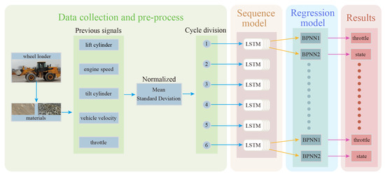
Figure 3.
The model presented in this paper.
Part one: Data collection and pre-processing. Neural networks require real driving data from the skilled operator to imitate the experienced operator. For the collection of wheel loader driving data, skilled drivers were required to perform a V-cycle in the actual working environment. To improve the computation speed and prediction accuracy, the driving data are normalized, and the working cycle is divided.
Part two: Sequence model. LSTM, which is capable of extracting temporal features and solving the problem of gradient disappearance in the original RNN, is applied in this paper. Six LSTM networks with the same structure are used for six stages of the working cycle.
Part three: Regression model. In order to output the final results, two BPNNs following the LSTM output of the prediction results of throttle value and state, respectively.
Each part is discussed in detail as follows.
3.2. Data Collection and Pre-Processing
The data acquisition of the wheel loader is shown in Figure 4, which is equipped with pressure sensors and GPS. Field data were collected in sites with dry ground. To study the adaptability of the proposed prediction approach, it is important to conduct experiments with a variety of materials. Small coarse gravel (SCG) and large coarse gravel (LCG) were used as the operating materials for this experiment, which are shown in Figure 5. Small coarse gravel mainly contains particles with sizes 0–25 mm, while large coarse gravel mainly contains particles with sizes 25–500 mm.
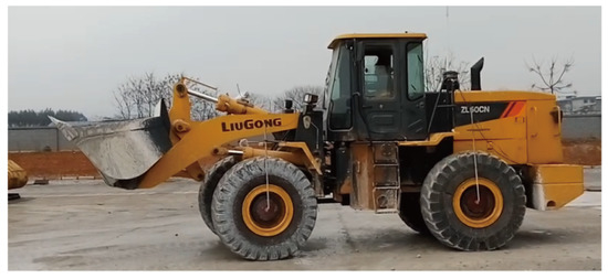
Figure 4.
Experimental wheel loader.
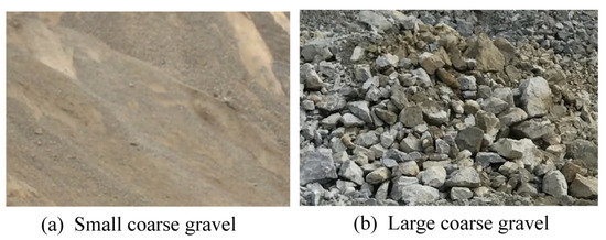
Figure 5.
Two operating materials.
The V-cycle of wheel loaders consists of six working phases, which possess their own unique characteristics. To improve the prediction precision and computation efficiency, six prediction models were constructed for six phases of the working cycle of wheel loaders. Normalization was used to speed up the training. According to the working characteristics of wheel loaders in the V-cycle, the V-cycle was divided by extracting the working condition features of the actuator and walking device to realize the mapping between the collected data and working state, as shown in Figure 6. For different operating materials, 50 sets of data were collected to train and test the prediction model.
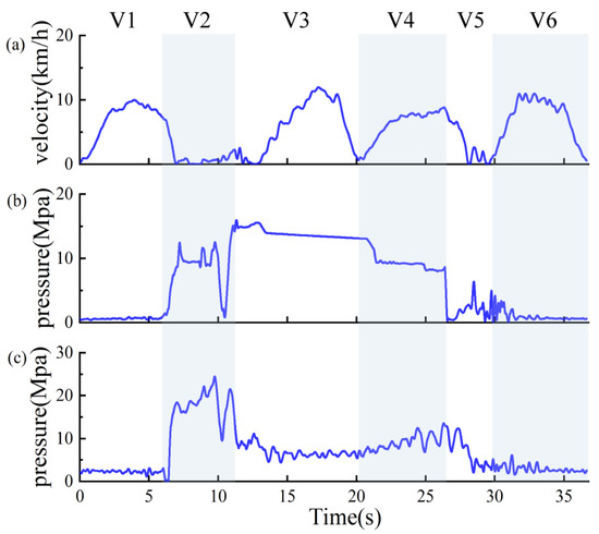
Figure 6.
Schematic diagram of working condition division: (a) velocity of wheel loader; (b) lift cylinder pressure; (c) tilt cylinder pressure.
3.3. Construction of LSTM
The proposed deep-learning-based prediction method consists of LSTM and BPNN, as illustrated in Figure 7. LSTM can memorize the temporal relationship in time-series data. The particular gate structure of the LSTM allows the networks to learn when to store and when to forget the relationship. Thus, the temporal information of the driving data is encoded into the LSTM network. In the training process, the high-dimensional temporal information was extracted by the hidden layer from the time-series data.
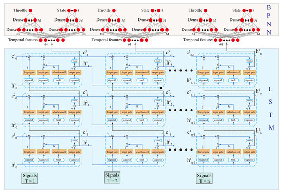
Figure 7.
Structure of the proposed LSTM and BPNN.
The LSTM model is developed with triple-stacked LSTM units because this configuration outperformed the double-stacked and the single-stacked LSTM in the training experiment. Meanwhile, compared with quadruple-stacked LSTM, triple-stacked LSTM has similar prediction precision and requires fewer computation resources. This result implies that increasing the structural complexity of the LSTM does not always lead to an improvement in the prediction accuracy.
The prediction of throttle value and state share an LSTM network to extract the temporal features. An alternative option is to use two LSTMs to extract the temporal features and predict the throttle value and state separately. However, two LSTMs introduce the extra burden of training and real-time calculations. In the experiment, both options have a similar effect. A possible explanation for this is that the sequence features required to predict the throttle value and state are similar.
When operators drive wheel loaders to work, the cycle operation time is diverse. Thus, the time-series data have different lengths. For the LSTM network, the time-series data with different sequence lengths need padding to ensure the same length. However, after padding for the time-series data, the prediction ability of the network will be influenced. Therefore, in this paper, the batch-size was set to 1 to ensure prediction accuracy.
The time-series data were taken as the input and the time dimension was [1,2,…t,…n]. each sequence has five parameters: lift cylinder, tilt cylinder, engine speed, vehicle velocity and throttle, respectively. In the training process, all previous throttle values and state values were taken as the inputs to output the corresponding prediction values of the next moment via BPNN, and the real values of the next moment were used as the correct mark values.
For the LSTM, the number of output units is 64. To train the neural networks, the learning rate was 0.001, while the loss function was mean squared error (MSE) and expressed as:
where and are, respectively, the predicted value and the actual value of the sampling point in the test set, and N is the number of samples in the test set.
The solver was the Adam algorithm [39], which is one of the most common solvers and suitable for training RNN. To assess the quality of training results, the root mean square error (RMSE) is taken as the criterion and expressed as:
3.4. Construction of BPNN
Two BPNNs with 64 inputs were used to output the prediction results of throttle value and state. The temporal information extracted from all previous data was taken as the input parameter of BPNN at each moment and the BPNN output the prediction values of the next moment. The two BPNNs have the same structure, with two hidden layers, with 64 and 32 units, respectively. The BPNN structure was proven to be effective and accurate. The BPNN part in Figure 4 depicts the network architecture. The Rectified Linear Units were chosen as the activation function of BPNN because they allow for deep neural networks to be trained with acceptable speed and performance [40].
4. Results and Discussion
TensorFlow was employed for the programming implementation of the benchmark and proposed architectures. The time-series data were imported into Python as a list. The label was placed in the other list. The first 40 elements of the lists were used as the training set, and the last 10 elements formed the test set.
4.1. Performance Analysis of Deep Learning Model for Different Materials
To validate the adaptability of the proposed method on the prediction problem, the experimental wheel loader was required to load different materials with the V-cycle operation mode at two different working sites, and the collected driving data at the two test sites were used as the inputs to train two LSTM network individually. Meanwhile, the throttle value and state of the wheel loader at the next time step were used as the output to train the networks. In addition to the different operating materials, the two different working sites have different driving road surfaces. When loading small coarse gravel, the pavement comprised concrete road surfaces, and when loading large coarse gravel, the pavement comprised native soil road surfaces. For each working material, 50 sets of driving data were collected at a 200 Hz sampling frequency. The data were further divided into training data, consisting of 40 sets, and testing data, consisting of 10 sets.
Figure 8 shows the comparison results of the RMSE of the predicted throttle value and state using small and large coarse gravel as working materials for the six working stages and 10 groups of test data, respectively. Each boxplot represents the quartiles of RMSE, where the current throttle value and state are used as the input, and the prediction results belong to the next time step. It can be seen from Figure 8a that the RMSE of the predicted throttle value for two different materials was less than 1.8 and, compared with the RMSE using small coarse gravel as working materials, the RMSE using large coarse gravel had a higher mean and wider variation range, which indicates worse prediction results. In Figure 8b, the RMSE of the predicted state for two different materials are less than 5, with the same comparison results as the predicted throttle value. A possible explanation for this is that the complexity of working environments has an impact on prediction accuracy. If large coarse gravel is used as the working material, the load of the wheel loader will change drastically during the bucket-filling stage (V2) and dumping stage (V5), which increases the difficulty of prediction. In addition to this, native soil pavement is more complicated than concrete pavement, so the interaction between the wheel loader and the environment has stronger randomness. The predicted results and the actual values under two different working conditions are compared in Figure 9. As shown in Figure 9, during the whole working cycle, the LSTM network can predict the throttle value and state with relatively high accuracy under different working conditions, which means that the proposed prediction model has good adaptability.
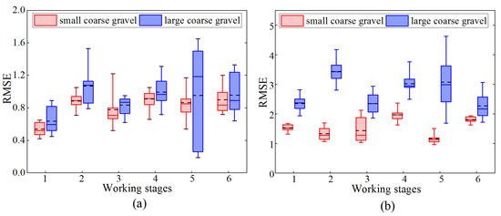
Figure 8.
Comparison of RMSE from different materials: (a) prediction of throttle value (b) prediction of state. mean and median values are shown with ‘–’ and ‘—’ respectively.
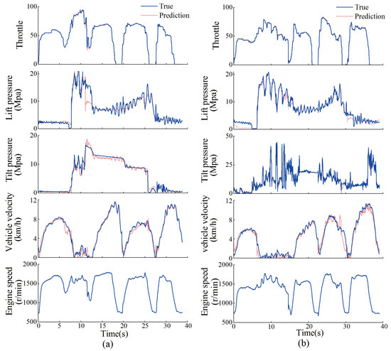
Figure 9.
Driving data of experienced drivers and the predicted value from different materials: (a) small coarse gravel (b) large coarse gravel.
4.2. Comparison with Different Deep Learning Models
The single V-cycle of wheel loaders consists of six stages, which have different operation modes and feature data. To more accurately extract unique feature data for each work stage and obtain high prediction accuracy, six LSTM prediction networks are developed for different stages. A single LSTM prediction network can also be used for this work. A single prediction network takes the complete data containing six stages as input and outputs the prediction result, which is end-to-end deep learning. End-to-end deep learning can reduce the hand-designed features and intermediate steps, but requires a considerable amount of data.
Figure 10 compares the RMSE results of the single LSTM prediction network and multiple LSTM prediction networks using small coarse gravel (SCG) as a working material. From Figure 10, it can be seen that the RMSE obtained by the single prediction networks has a higher mean and wider variation range compared with the RMSE obtained by the multiple prediction networks. Particularly for the bucket-filling stage (V2) and dumping stage (V5), the multiple prediction networks significantly outperforms the single prediction network in the prediction effect. The above finding can be further confirmed by Figure 11, which shows the RMSE comparison results using large coarse gravel (LCG) as a working material. There are two possible reasons for this result. The first reason is that there is a change in the load of the wheel loader during the bucket-filling stage and the dumping stage. The lift and tilt of the working device also account for this result. Therefore, in the case of limited data, to obtain accurate prediction results, it is necessary to establish different prediction networks for different working stages. However, it should be noted that the single prediction network may achieve the same performance as the multiple prediction networks with sufficient data.
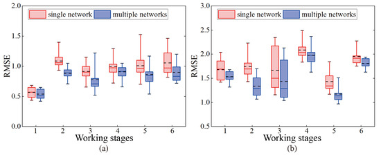
Figure 10.
RMSE comparison of different LSTM networks using small coarse gravel: (a) prediction of throttle value (b) prediction of state.
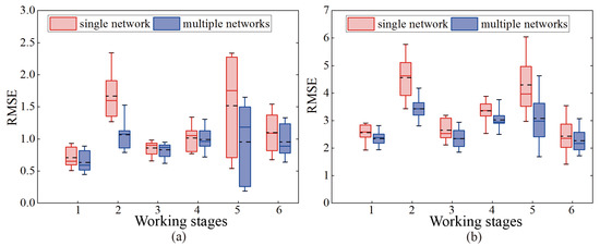
Figure 11.
RMSE comparison of different LSTM networks using large coarse gravel: (a) prediction of throttle value (b) prediction of state.
BPNN is also used as a benchmark model for different stages. Figure 12 and Figure 13 compare the RMSE results of BPNNs and LSTM networks. The result shows that the LSTM network has a better prediction effect. The better prediction result can be ascribed to the fact that LSTM can extract temporal features, which can make the model understand the environment and wheel loader more accurately. The RMSE of throttle value for different operating materials and models is shown in Table 2, and the RMSR of state is shown in Table 3.
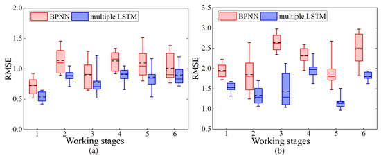
Figure 12.
RMSE comparison of BPNNs and LSTM networks using small coarse gravel: (a) prediction of throttle value (b) prediction of state.
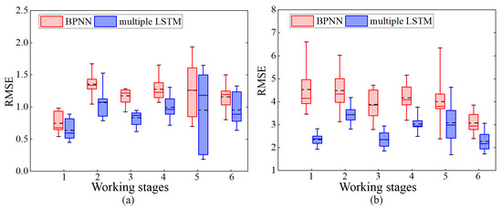
Figure 13.
RMSE comparison of BPNNs and LSTM networks using large coarse gravel: (a) prediction of throttle value (b) prediction of state.
Table 2.
The RMSE of throttle value for different operating materials and models.
Table 3.
The RMSE of state for different operating materials and models.
4.3. Performance Analysis of LSTM Networks for Different Sampling Frequency
Due to the high integration of the wheel loader and the high signal density, the sampling frequency is severely restricted by the storage capacity of the host. The appropriate sampling frequency should be as low as possible while ensuring prediction accuracy. The low sampling frequency can reduce the amount of data, thereby reducing the cost of data storage and the consumption of computation resources. Therefore, to reduce the cost, it is necessary to study the relationship between the signal sampling frequency and the prediction accuracy. The sampling frequency is reduced to 100, 50, 20, and 10 Hz, respectively.
Figure 14 and Figure 15 show the relationship between prediction performance and signal sampling frequency. Table 4 shows the RMSE of throttle value and state under different sampling frequencies. It can be seen that the prediction effect improves with the increase of the signal sampling frequency. This result may be explained by the fact that the higher sampling frequency can provide sufficient feature information in time. However, the too-high sampling frequency may bring more noise, making it difficult for the neural network model to learn the correct mapping from input to output. At the same time, when the sampling frequency is higher than 50 Hz, the increase in frequency does not significantly improve the prediction performance. In practice, although the increase in sampling frequency will improve the prediction accuracy, it will also lead to an increase in storage costs and a decrease in the real-time calculation rate. Therefore, a trade-off is necessary for the selection of sampling frequency. For example, if a fully automated system is required, a higher sampling frequency is necessary to reduce the prediction error. However, for the assisted driving, a lower sampling frequency should be considered to reduce the storage and computing costs.
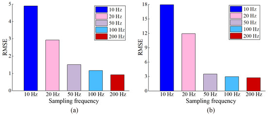
Figure 14.
Relationship between sampling frequency and prediction performance using large coarse gravel: (a) prediction of throttle value (b) prediction of state.
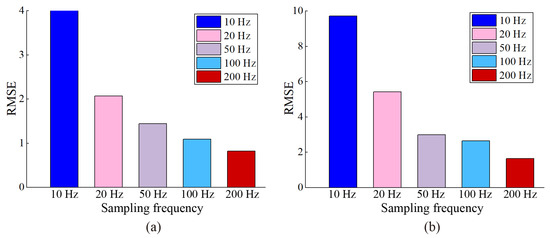
Figure 15.
Relationship between sampling frequency and prediction performance using small coarse gravel: (a) throttle prediction (b) state prediction.
Table 4.
The RMSE of throttle value and state under different sampling frequency.
5. Conclusions
This paper proposed a deep-learning-based method to predict throttle value and state for wheel loaders. The prediction model can help achieve autonomous operation and reduce the need for remote intervention during remote operation. Additionally, the proposed model can be applied to model predictive control and energy management to achieve a good performance in terms of efficiency and fuel consumption.
The prediction model consists of three main parts, namely, data collection and pre-processing, LSTM and BPNN. Six LSTM networks are used to extract the temporal features of six stages of the V-cycle for wheel loaders. Based on the extracted temporal features, two BPNNs are employed to predict the throttle value and state of wheel loaders, respectively. The data obtained from two different working materials and pavements are used to train and test the proposed prediction model. The results show that the proposed prediction model can achieve a good prediction effect under different working conditions and outperform BPNNs. Moreover, compared with end-to-end deep learning, which only uses a single LSTM network for prediction, the prediction model of multiple LSTM networks shows better prediction performance. However, the prediction model of multiple neural networks requires more hand-designed features. The relationship between signal sampling frequency and prediction accuracy is also studied. In the range of 10 Hz to 200 Hz, as the frequency increases, the prediction performance improves. However, when the signal sampling frequency exceeds 50 Hz, the improvement effect of prediction accuracy is not obvious as the frequency increases. Therefore, in engineering practice, it is necessary to weigh the prediction accuracy and cost. Although this paper takes the wheel loader as the research object, the proposed prediction model can be adapted to other construction machinery. In future, the prediction network will be deployed to a physical wheel loader to improve the efficiency and real-time fuel efficiency using reinforcement learning.
Author Contributions
Conceptualization, J.H. and X.C.; methodology, J.H. and Y.S.; software, J.H. and X.C.; validation, J.H. and Y.S.; formal analysis, D.K.; investigation, X.C.; resources, J.W.; data curation, Y.S. and X.C.; writing—original draft preparation, J.H.; writing—review and editing, J.W. and D.K.; visualization, X.C. and Y.S.; supervision, J.W.; project administration, J.W.; funding acquisition, J.W. and D.K. All authors have read and agreed to the published version of the manuscript.
Funding
This research was funded by the National Natural Science Foundation of China grant number 51875239.
Institutional Review Board Statement
Not applicable.
Informed Consent Statement
Not applicable.
Conflicts of Interest
The authors declare no conflict of interest.The funders had no role in the design of the study; in the collection, analyses, or interpretation of data; in the writing of the manuscript, or in the decision to publish the results.
References
- Davila Delgado, J.M.; Oyedele, L.; Ajayi, A.; Akanbi, L.; Akinade, O.; Bilal, M.; Owolabi, H. Robotics and automated systems in construction: Understanding industry-specific challenges for adoption. J. Build. Eng. 2019, 26, 100868. [Google Scholar] [CrossRef]
- Frank, B.; Kleinert, J.; Filla, R. Optimal control of wheel loader actuators in gravel applications. Autom. Construct. 2018, 91, 1–14. [Google Scholar] [CrossRef]
- Hemami, A.; Hassani, F. An overview of autonomous loading of bulk material. Int. Symp. Autom. Rob. Constr. 2009, 405–411. [Google Scholar] [CrossRef]
- Dadhich, S.; Bodin, U.; Sandin, F.; Andersson, U. From Tele-Remote Operation to Semi-Automated Wheel-Loader. Int. J. Electr. Electron. Eng. Telecommun. 2018, 178–182. [Google Scholar] [CrossRef][Green Version]
- Hemami, A. Fundamental Analysis of Automatic Excavation. J. Aerosp. Eng. 1995, 8, 175–179. [Google Scholar] [CrossRef]
- Bobbie, F.; Lennart, S.; Reno, F.; Anders, F. On Increasing Fuel Efficiency by Operator Assistant Systems in a Wheel Loader. In Proceedings of the International Conference on Advanced Vehicle Technologies and Integration (VTI 2012), Changchun, China, 16–19 July 2012; pp. 155–161. [Google Scholar]
- Roberts, J.M.; Duff, E.S.; Corke, P.I. Reactive navigation and opportunistic localization for autonomous underground mining vehicles. Inf. Sci. 2002, 145, 127–146. [Google Scholar] [CrossRef]
- Dadhich, S.; Bodin, U.; Andersson, U. Key challenges in automation of earth-moving machines. Autom. Construct. 2016, 68, 212–222. [Google Scholar] [CrossRef]
- Marshall, J.A.; Murphy, P.F.; Daneshmend, L.K. Toward Autonomous Excavation of Fragmented Rock: Full-Scale Experiments. IEEE Trans. Autom. Sci. Eng. 2008, 5, 562–566. [Google Scholar] [CrossRef]
- Sotiropoulos, F.E.; Asada, H.H. A Model-Free Extremum-Seeking Approach to Autonomous Excavator Control Based on Output Power Maximization. IEEE Robot. Autom. Lett. 2019, 4, 1005–1012. [Google Scholar] [CrossRef]
- Dobson, A.A.; Marshall, J.A.; Larsson, J. Admittance Control for Robotic Loading: Design and Experiments with a 1-Tonne Loader and a 14-Tonne Load-Haul-Dump Machine. J. Field Robot. 2017, 34, 123–150. [Google Scholar] [CrossRef]
- Dadhich, S.; Sandin, F.; Bodin, U.; Andersson, U.; Martinsson, T. Field test of neural-network based automatic bucket-filling algorithm for wheel-loaders. Autom. Construct. 2019, 97, 1–12. [Google Scholar] [CrossRef]
- Sun, W.; Iwataki, S.; Komatsu, R.; Fujii, H.; Yamashita, A.; Asama, H. Simultaneous tele-visualization of construction machine and environment using body mounted cameras. In Proceedings of the 2016 IEEE International Conference on Robotics and Biomimetics (ROBIO), Qingdao, China, 3–7 December 2016; pp. 382–387. [Google Scholar] [CrossRef]
- Yamada, H.; Muto, T. Development of a Hydraulic Tele-Operated Construction Robot using Virtual Reality. Int. J. Fluid Power 2003, 4, 35–42. [Google Scholar] [CrossRef]
- Fernando, C.L.; Saraiji, M.Y.; Seishu, Y.; Kuriu, N.; Minamizawa, K.; Tachi, S. Effectiveness of Spatial Coherent Remote Drive Experience with a Telexistence Backhoe for Construction Sites. In Proceedings of the ICAT-EGVE, Kyoto, Japan, 28–30 October 2015; pp. 69–75. [Google Scholar]
- Feng, H.; Yin, C.; Ma, W.; Yu, H.; Cao, D. Parameters identification and trajectory control for a hydraulic system. ISA Trans. 2019, 92, 228–240. [Google Scholar] [CrossRef]
- Yoo, S.; Park, C.G.; You, S.H.; Lim, B. A Dynamics-Based Optimal Trajectory Generation for Controlling an Automated Excavator. Proc. Inst. Mech. Eng. Part C-J. Eng. Mech. Eng. Sci. 2010, 224, 2109–2119. [Google Scholar] [CrossRef]
- Zou, Z.; Chen, J.; Pang, X. Task space-based dynamic trajectory planning for digging process of a hydraulic excavator with the integration of soil–bucket interaction. Proc. Inst. Mech. Eng. Part K-J. Multi-Body Dyn. 2018, 233, 598–616. [Google Scholar] [CrossRef]
- Bauza, M.; Hogan, F.R.; Rodriguez, A. A Data-Efficient Approach to Precise and Controlled Pushing. In Proceedings of the Conference on Robot Learning, Zürich, Switzerland, 29–31 October 2018; pp. 336–345. [Google Scholar]
- Byravan, A.; Fox, D. SE3-nets: Learning rigid body motion using deep neural networks. In Proceedings of the 2017 IEEE International Conference on Robotics and Automation (ICRA), Singapore, 29 May–3 June 2017; pp. 173–180. [Google Scholar] [CrossRef]
- Sotiropoulos, F.E.; Asada, H.H. Autonomous Excavation of Rocks Using a Gaussian Process Model and Unscented Kalman Filter. IEEE Robot. Autom. Lett. 2020, 5, 2491–2497. [Google Scholar] [CrossRef]
- Sandzimier, R.J.; Asada, H.H. A Data-Driven Approach to Prediction and Optimal Bucket-Filling Control for Autonomous Excavators. IEEE Robot. Autom. Lett. 2020, 5, 2682–2689. [Google Scholar] [CrossRef]
- Koo, B.; La, S.; Cho, N.W.; Yu, Y. Using support vector machines to classify building elements for checking the semantic integrity of building information models. Autom. Construct. 2019, 98, 183–194. [Google Scholar] [CrossRef]
- Hasan, M.A.M.; Ahmad, S.; Molla, M.K.I. Protein subcellular localization prediction using multiple kernel learning based support vector machine. Mol. Biosyst. 2017, 13, 785–795. [Google Scholar] [CrossRef]
- Shi, Y.; Xia, Y.; Zhang, Y.; Yao, Z. Intelligent identification for working-cycle stages of excavator based on main pump pressure. Autom. Construct. 2020, 109. [Google Scholar] [CrossRef]
- Li, Y.; Xu, M.; Wei, Y.; Huang, W. A new rolling bearing fault diagnosis method based on multiscale permutation entropy and improved support vector machine based binary tree. Measurement 2016, 77, 80–94. [Google Scholar] [CrossRef]
- Arabi, S.; Haghighat, A.; Sharma, A. A deep-learning-based computer vision solution for construction vehicle detection. Comput.-Aided Civil. Infrastruct. Eng. 2020, 35, 753–767. [Google Scholar] [CrossRef]
- Park, J.; Lee, B.; Kang, S.; Kim, P.Y.; Kim, H.J. Online Learning Control of Hydraulic Excavators Based on Echo-State Networks. IEEE Trans. Autom. Sci. Eng. 2017, 14, 249–259. [Google Scholar] [CrossRef]
- Kim, J.; Chi, S. Action recognition of earthmoving excavators based on sequential pattern analysis of visual features and operation cycles. Autom. Construct. 2019, 104, 255–264. [Google Scholar] [CrossRef]
- Yao, Z.; Huang, Q.; Ji, Z.; Li, X.; Bi, Q. Deep learning-based prediction of piled-up status and payload distribution of bulk material. Autom. Construct. 2021, 121. [Google Scholar] [CrossRef]
- Luo, H.; Wang, M.; Wong, P.K.Y.; Tang, J.; Cheng, J.C.P. Construction machine pose prediction considering historical motions and activity attributes using gated recurrent unit (GRU). Autom. Construct. 2021, 121. [Google Scholar] [CrossRef]
- Shi, J.; Sun, D.; Hu, M.; Liu, S.; Kan, Y.; Chen, R.; Ma, K. Prediction of brake pedal aperture for automatic wheel loader based on deep learning. Autom. Construct. 2020, 119. [Google Scholar] [CrossRef]
- Xing, Y.; Lv, C.; Mo, X.; Hu, Z.; Huang, C.; Hang, P. Toward Safe and Smart Mobility: Energy-Aware Deep Learning for Driving Behavior Analysis and Prediction of Connected Vehicles. IEEE Trans. Intell. Transp. Syst. 2021, 22, 4267–4280. [Google Scholar] [CrossRef]
- Dai, S.; Li, L.; Li, Z. Modeling Vehicle Interactions via Modified LSTM Models for Trajectory Prediction. IEEE Access 2019, 7, 38287–38296. [Google Scholar] [CrossRef]
- Fang, W.; Ding, L.; Zhong, B.; Love, P.E.D.; Luo, H. Automated detection of workers and heavy equipment on construction sites: A convolutional neural network approach. Adv. Eng. Inform. 2018, 37, 139–149. [Google Scholar] [CrossRef]
- Kim, J.; Chi, S.; Seo, J. Interaction analysis for vision-based activity identification of earthmoving excavators and dump trucks. Autom. Construct. 2018, 87, 297–308. [Google Scholar] [CrossRef]
- Zhang, S.; Yao, L.; Sun, A.; Tay, Y. Deep Learning Based Recommender System: A Survey and New Perspectives. ACM Comput. Surv. 2019, 52, 1–38. [Google Scholar] [CrossRef]
- Hochreiter, S.; Schmidhuber, J. Long short-term memory. Neural Comput. 1997, 9, 1735–1780. [Google Scholar] [CrossRef]
- Kingma, D.P.; Ba, J.L. Adam: A Method for Stochastic Optimization. arXiv 2018, arXiv:1412.6980. [Google Scholar]
- Nair, V.; Hinton, G.E. Rectified linear units improve Restricted Boltzmann machines. In Proceedings of the ICML, Haifa, Israel, 21–24 June 2010; pp. 807–814. [Google Scholar]
Publisher’s Note: MDPI stays neutral with regard to jurisdictional claims in published maps and institutional affiliations. |
© 2021 by the authors. Licensee MDPI, Basel, Switzerland. This article is an open access article distributed under the terms and conditions of the Creative Commons Attribution (CC BY) license (https://creativecommons.org/licenses/by/4.0/).