Hybrid Controller Based on LQR Applied to Interleaved Boost Converter and Microgrids under Power Quality Events

Abstract

Renewable energy sources are an environmentally attractive idea, but they require a proper control scheme to guarantee optimal operation. In this work, we tune different controllers for an Interleaved Boost Converter (IBC) powered by a photovoltaic array using three metaheuristics: Genetic Algorithm, Particle Swarm Optimization, and Gray Wolf Optimization. We also develop several controllers for a second simulated scenario where the IBC is plugged into an existing microgrid (MG) as this can provide relevant data for real-life applications. In both cases, we consider hybrid controllers based on a Linear Quadratic Regulator (LQR). However, we hybridize it with an Integral action (I-LQR) in the first scenario to compare our data against previously published controllers. In the second one, we add a Proportional-Integral technique (PI-LQR) as we do not have previous data to compare against to provide a more robust controller than I-LQR. To validate our approach, we run extensive simulations with each metaheuristic and compare the resulting data. We focus on two fronts: the performance of the controllers and the computing cost of the solvers when facing practical issues. Our results demonstrate that the approach proposed for tuning controllers is a feasible strategy. The controllers tuned with the metaheuristics outperformed previously proposed strategies, yielding solutions thrice faster with virtually no overshoot and a voltage ripple seven times smaller. Not only this, but our controllers could correct some issues liaised to the IBC when it is plugged into an MG. We are confident that these insights can help migrate this approach to a more diverse set of MGs with different renewable sources and escalate it to real-life experiments.

1. Introduction

Recent studies have corroborated that the excessive exploitation of fossil fuels as a primary energy source has caused negative impacts on our environment. Nonetheless, experts recognize energy consumption as a pillar of worldwide economic development. Therefore, environmental organizations have encouraged the exploration of alternative and sustainable energy sources. The chief goal is to update the current electrical system by incorporating renewable energies so that fossil fuel consumption can be gradually decreased to 20% by 2050 [1]. This objective has created several research opportunities in the Distributed Energy Resources (DERs) field. Some examples include the technological furthering of power electronics for energy production, as well as the challenges associated with energy quality, electric power systems reliability, and increasing energy demand. The DERs appear as an innovative solution that benefits customers at a lower energetic cost while preserving a high power quality and energy independence [2]. Moreover, integrating DERs with green technologies (e.g., wind, geothermal, biomass, and hydroelectric) can help in reducing the carbon footprint and generate a self-sustaining power system. Because of this, the development of Microgrids (MG) based on DERs with clean power technology has attracted increased attention from both the scientific community and energy consumers (buildings, factories, and communities). MGs and DERs have similar features. Some of them include their reliability and enhancement of energy quality, as well as their decarbonization and decentralization of the electrical grid [3]. Additionally, an MG is defined as a group of interconnected loads and DERs with clearly defined electrical boundaries that function as a controllable entity regarding the utility grid [4].

In general terms, an oscillatory power signal is provoked by unbalanced loads (either linear or nonlinear). Such signals flow through the Voltage Source Inverter (VSI) until the Point of Common Coupling (PCC) between the MG and the utility grid, compromising the system reliability. Bear in mind that the PCC is well known as the interface between the MG and the electrical grid. Additionally, the VSI synthesizes some MG components, such as the renewable energy source and the three-phase inverter. These elements are modeled as an ideal voltage source. Now, one way to analyze abnormalities within power signals injected by an MG is to use the symmetrical components method [5]. With it, one can analyze a system under normal or unbalanced conditions. In this sense, it is possible to detect the negative-sequence components of the signals delivered by the MG, altering voltage equilibrium at PCC through the well-known Voltage Unbalanced Factor (VUF) described in the IEEE 1159–2019 standard [6]. Conversely, harmonics are additional signals of current or voltage that manifest within a power signal as the multiples of the system fundamental frequency. In an electric power system, harmonic content can be introduced by nonlinear loads. This phenomenon distorts the waveforms of signals delivered by the MG, so it is paramount not to exceed the Total Harmonic Distortion limit (THD) established in the International Electrotechnical Commission Standard (IEC) [7].

There have been diverse attempts at achieving MG controllers with small DC source inputs that perform properly [8,9]. The Interleaved Boost Converter (IBC) is one such alternative. This alternative can be integrated into the structure of an MG, allowing for an increased voltage from the renewable source. Following the selected topology for the IBC, we can note that the input current is divided among the switches connected in parallel. This scheme augments the reliability and efficiency of the converter, w.r.t. the Boost Converter (BC). Besides, by adjusting the duty cycle appropriately, one can mitigate ripples within the input current all the way down to zero. Furthermore, output filters for IBCs are smaller than those for BCs, which minimizes losses and current stress for the power switches [10]. This effect leads to a stable power supply with the desired control response. Huangfu et al. found that a two-phase DC-DC IBC is a suitable option with high efficiency and fast dynamics, which can be used in high power density applications [11].

The IBCs have been mostly applied for improving the management of Proton Exchange Membrane Fuel Cells (PEMFCs) [12,13]. A relevant example is the work of Ahmadi et al. [14], where the authors proposed tuning a PID controller with the Particle Swarm Optimization (PSO). They controlled the Maximum Power Point Tracker (MPPT) of PEMFCs by adjusting the duty cycle. The authors compared their data against that yielded by the Perturb and Observe (P&O) and Sliding Mode (SM) algorithms, finding that their proposed approach exhibited a high precision under MPPT power fluctuations.

In other control schemes, Habib and Khoucha. [15] compared the performance between the LQR algorithm and the classical PI controller under current undulation and load, as well as voltage variations. Similarly, Habib et al. [10] used Genetic Algorithm (GA) to optimize the parameters of LQR controllers and quantify performance metrics given by the overshoot, response time, and ripple reduction. Another interesting approach related to controllers tuned by MHs is the work proposed by Banerjee et al. [16]. In their work, authors compared the efficiency between classical and optimal Type-III controllers. Besides, they proposed a comparative study among IBCs and BCs, considering both kinds of controllers. Cao et al. [17] also worked on tuning LQR controllers. However, they employed an improved version of the Chaotic Whale Optimization Algorithm and sought to preserve PEMFCs within the desired operating range. Even so, they analyzed similar metrics (ripple and overshoot) while comparing their data against previous works. This study demonstrated that Metaheuristics (MHs) are powerful tools for tuning LQR, classical, and hybrid controllers. In fact, hybrid controllers stand as a suitable choice when one wants a fast response with good energy efficiency, i.e., robust and tolerant to perturbations. For example, Kim et al. [18] proposed a controller offering a low operation cost and a reduced error, which they called LQR+PI.

Controlling schemes have also been used for improving MG performance. Savaghebi et al. [19] designed a hierarchical control for improving the voltage quality of sensitive loads connected to the AC bus. The authors proposed a two-level controlling scheme. The former managed DERs while the latter balanced voltage and harmonics. Dasgupta et al. [20] implemented a new current control technique. They considered a three-phase framework for active and reactive power flow management from a renewable energy source.

Moreover, system stability was ensured by including the Lyapunov function. Such a control scheme was focused on reducing the THD generated by typical nonlinear loads. Throughout the same year, Lotfollahzade et al. [21] presented an LQR controller for compensating unbalanced nonlinear loads in grid-tied and island mode. They included a PID controller tuned by PSO, which managed the load from a set of distributed generators. A few years later, Shi et al. [22] enhanced the MG power quality and the inverter performance using a negative-sequence compensation method. Later on, Mousavi et al. [23] adopted a resonant control strategy based on active and reactive power controllers. With this, they compensated power quality problems at the Distributed Generation (DG) terminals or the PCC.

Then, Hadidian et al. [24] tested a control scheme applied to four-leg battery energy storage systems called BESS. Here, the authors considered an MG operating in isolated mode faced with unbalanced and nonlinear loads. This approach exhibited a reduced steady-state error, a fast transient response, and a low THD index. Beus et al. [25] presented a hierarchical control method with three levels for MGs operating in grid-tied mode. The first level minimized the MG operating cost. The second level used a predictive controller and a Kalman filter for controlling the frequency of the MG. Finally, the third level used classical controllers for tracking the set-points coming from the previous levels. Faria et al. [26] proposed a new method for determining the optimal parameters of the proportional resonant controller, as well as the values of the output filter upon a grid-tied three-phase inverter through the Gray Wolf Optimization (GWO). The authors designed the fitness function based on harmonic attenuation rate, power loss, and steady-state error reduction. Additionally, Ebrahim et al. [27] compared three MHs techniques to properly select the resonant proportional controller and its harmonic compensator for three-phase voltage source inverters connected to the electrical grid. They employed a multi-objective function for minimizing the harmonic distortion of the grid output current.

Despite their broad use for MG-related applications, hybrids between LQR and PID controllers are also widespread in other engineering applications. For example, Nagarkar et al. [28] tackled the nonlinear model of a quarter car suspension system, where the controller was driven by a GA. Lindiya et al. [29] followed an equivalent approach, but they applied it to improve the performance of DC-DC converters. Similarly, Şen and Kalyoncu [30] used the GWO for tuning the controller. The authors, however, used this approach for regulating the foot trajectory of a quadruped robot. Moreover, Ibrahim and Abdulla explored the stabilization of a helicopter with three degrees of freedom [31].

It is well-known that the nature of an IBC is highly nonlinear. Even so, most of the control schemes proposed for the IBC dynamic are linear. In this sense, we followed a similar approach. As proposed in [10,17], we linearized the IBC mathematical model considering the duty cycle of inductors and the system equilibrium points. However, bear in mind that even if this facilitates model decoupling, it has the drawback of lowering performance due to the non-minimum phase problem Banerjee et al. [16]. Nonetheless, there are several works dealing with this issue, as was mentioned above. However, the performance of such controllers still has room for improvement. Besides, most previous works either deal with PEMFCs or consider photovoltaic (PV) cells that are directly connected to the MG. Moreover, the earlier approaches consider ideal elements, which obscures performance in real-life applications.

In this work, we propose two approaches. The first one deals with tuning IBC controllers in standalone mode by considering a multi-input single-output control path. We focus on the settling time, overshoot, and steady-state error, as well as on the response when faced with perturbations, and the output voltage ripple. Likewise, we design a hybrid I-LQR controller driven by metaheuristics. Through it, we seek to improve the aforementioned metrics. Moreover, we consider photovoltaic cells as the energy source connected to the IBC.

As for the second approach, we introduce a new methodology for adjusting MG control parameters when handling power quality issues, which is powered by metaheuristics. In this case, we incorporate a PI-LQR controller, which contemplates the same control specifications as in the first approach. Besides, we tackle the specific case of power exchange between IBC and VSI, where energy is supplied by an MG towards the loads connected at the PCC. Note that the IBC is seen as an ideal voltage source within the MG model. Besides, drawbacks related to power quality in the MG are generated by unbalanced linear and nonlinear loads. In this approach, the IBC feeds the MG while the latter works in grid-tied mode and thus conforming the IBC+MG set.

To power our approach, we selected the most popular algorithms in the last few years. We determined them by analyzing previously reported applications. Our exploration revealed approaches where Particle Swarm Optimization (PSO) and Genetic Algorithms (GA) were used to tune IBC controllers [10,16,17]. We also detected reports about the successful application of the Grey Wolf Optimizer (GWO) for adjusting control parameters in microgrids [26,27].

In summary, our work has five significant contributions:

• It proposes a hybrid controller ensuring voltage equilibrium at the PCC, according to the regulations overseeing MGs, while reducing harmonic content from nonlinear loads connected to the PCC.
• It provides a comparison between three MHs for finding the best controller configuration in terms of the IBC and MG dynamics.
• It describes controller performance for an IBC connected to VSI while the MG is working in grid-tied mode.
• It delivers different controller proposals that outperform recent developments from relevant literature while using photovoltaic cells as an energy source.
• It introduces a testing scenario closer to reality, which includes non-ideal elements such as voltage sources.

2. Fundamentals

2.1. Interleaved Boost Converter Model

An Interleaved Boost Converter (IBC) is a device used to increase the input voltage. They are quite useful for applications such as electric vehicles and voltage regulators in PEMFCs [17]. This kind of device preserves the working principle of a Boost Converter (BC). Furthermore, IBCs have remarkable advantages compared to BCs. Some of them include low ripple and harmonic content at the input and output current signals [16]. Such advantages match the power quality interest mentioned in this article. For this reason, we selected IBCs for this work. However, IBCs incorporate two inductance currents into their structure [10]. A feasible approach to construct an IBC is to connect two BC in parallel, resulting in a two-phase interleaved converter (Figure 1). In this case, it is paramount that the drive signals be shifted by ${180}^{°}$ [32].

Based on Figure 1, the mathematical model of an IBC depends on the activation of switches $Q_1$ and $Q_2$ and on the polarization of diodes $D_1$ and $D_2$. Bear in mind that R represents the load connected to the IBC. Accordingly, the IBC dynamic can be described in the state-space framework as

$$\begin{array}{c}\hfill \begin{array}{cc}\hfill \frac{d}{dt}\left(\begin{array}{c}{i}_{L_1}\\ i_{L_2}\\ v_{C_1}\end{array}\right)& =\left(\begin{array}{ccc}0& 0& s_1\\ 0& 0& s_2\\ s_3& s_4& -\frac{1}{R{C}_1}\end{array}\right)\left(\begin{array}{c}{i}_{L_1}\\ i_{L_2}\\ v_{C_1}\end{array}\right)+\left(\begin{array}{c}\frac{1}{L_1}\\ \frac{1}{L_2}\\ 0\end{array}\right)v_s,\hfill \\ \hfill & y=\left(\begin{array}{ccc}0& 0& 1\end{array}\right)\left(\begin{array}{c}{i}_{L_1}\\ i_{L_2}\\ v_{C_1}\end{array}\right),\hfill \end{array}\end{array}$$

(1)

where $s_k$, $\forall k=\{1,\cdots ,4\}$, are variables defined by the four possible operating modes shown in

Table 1. IBC activation modes that render different variants of (1).

Inputs				Outputs
${\mathit{Q}}_{\mathbf{1}}$	${\mathit{Q}}_{\mathbf{2}}$	${\mathit{D}}_{\mathbf{1}}$	${\mathit{D}}_{\mathbf{2}}$	${\mathit{s}}_{\mathbf{1}}$	${\mathit{s}}_{\mathbf{2}}$	${\mathit{s}}_{\mathbf{3}}$	${\mathit{s}}_{\mathbf{4}}$
1	1	0	0	0	0	0	0
1	0	0	1	0	$-\frac{1}{L_2}$	$\frac{1}{C_1}$	0
0	1	1	0	$-\frac{1}{L_1}$	0	$\frac{1}{C_1}$	0
0	0	1	1	$-\frac{1}{L_1}$	$-\frac{1}{L_2}$	$\frac{1}{C_1}$	$\frac{1}{C_1}$

.

Therefore, it is possible to obtain a weighted model of the IBC by adding a new input linked to the duty cycle of inductors ($U_1$ and $U_2$). However, this scheme leads to the following nonlinear mathematical model,

$$\left(\begin{array}{c}{f}_1\\ f_2\\ f_3\end{array}\right)=\frac{d}{dt}\left(\begin{array}{c}{i}_{L_1}\\ i_{L_2}\\ v_{C_1}\end{array}\right)=\left(\begin{array}{c}\frac{1}{L_1}\left(v_s-v_{C_1}{U}_1\right)\\ \frac{1}{L_2}\left(v_s-v_{C_1}{U}_2\right)\\ \frac{1}{C_1}\left(i_{L_1}{U}_1+i_{L_2}{U}_2\right)-\frac{v_{C_1}}{R{C}_1}\end{array}\right).$$

(2)

After averaging the IBC model one can infer that it is similar to the classical boost converter expression. However, bear in mind that the mathematical representation includes two inductor currents, as aforementioned. Therefore, the model expressed in (2) exhibits two commonplace scenarios for activation modes of the duty cycle: lower or higher than 50%. However, the duty cycle should be 50%, the IBC benefits from ripple reduction, either in the input current or in the capacitor voltage. Nonetheless, our approach does not restrict the values of these duty cycles.

As the proposed hybrid controller is based on a linear control technique, the nonlinear system must be linearized. This process can be done through the Jacobian obtained from the states x and inputs u,

$$\begin{array}{c}\hfill J_A=\frac{\partial }{\partial x}\left(\begin{array}{c}{f}_1\\ f_2\\ f_3\end{array}\right)\mathrm{and}{J}_B=\frac{\partial }{\partial u}\left(\begin{array}{c}{f}_1\\ f_2\\ f_3\end{array}\right),\end{array}$$

(3)

which derives into (4) and (5),

$$\begin{array}{c}\hfill J_A=\left(\begin{array}{ccc}\frac{\partial f_1}{\partial i_{L_1}}& \frac{\partial f_1}{\partial i_{L_2}}& \frac{\partial f_1}{\partial v_{C_1}}\\ \frac{\partial f_2}{\partial i_{L_1}}& \frac{\partial f_2}{\partial i_{L_2}}& \frac{\partial f_2}{\partial v_{C_1}}\\ \frac{\partial f_3}{\partial i_{L_1}}& \frac{\partial f_3}{\partial i_{L_2}}& \frac{\partial f_3}{\partial v_{C_1}}\end{array}\right)=\left(\begin{array}{ccc}0& 0& -\frac{U_1}{L_1}\\ 0& 0& -\frac{U_2}{L_2}\\ \frac{U_1}{C_1}& \frac{U_2}{C_1}& -\frac{1}{R{C}_1}\end{array}\right),\end{array}$$

(4)

$$\begin{array}{c}\hfill J_B=\left(\begin{array}{cc}\frac{\partial f_1}{\partial U_1}& \frac{\partial f_1}{\partial U_2}\\ \frac{\partial f_2}{\partial U_1}& \frac{\partial f_2}{\partial U_2}\\ \frac{\partial f_3}{\partial U_1}& \frac{\partial f_3}{\partial U_2}\end{array}\right)=\left(\begin{array}{cc}\frac{{\tilde{v}}_{C_1}}{L_1}& 0\\ 0& \frac{{\tilde{v}}_{C_1}}{L_2}\\ -\frac{{\tilde{i}}_{L_1}}{C_1}& -\frac{{\tilde{i}}_{L_2}}{C_1}\end{array}\right),\end{array}$$

(5)

where $\frac{d}{dt}{i}_{L_1}$ [A/s], $\frac{d}{dt}{i}_{L_2}$ [A/s], and $\frac{d}{dt}{v}_{C_1}$ [V/s] are related to the voltage at both inductors ($L_1$ [H], $L_2$ [H]) and to the current of the capacitor ($C_1$ [F]), respectively. Similarly, $i_{L_1}$ [A] and $i_{L_2}$ [A] stand for the current at the inductors and $v_{C_1}$ [V] is the voltage of the capacitor. As R represents the load connected to the IBC, it is connected to the output of the IBC and can be used as a comparison point against previous approaches. $v_s$ [V] is the input voltage source representing the PV modules, while $U_{d_1}$ and $U_{d_2}$ are the added system inputs (Duty Cycles). The final IBC model is obtained by inserting the equilibrium point,

$$\begin{array}{c}\hfill \left(\begin{array}{c}{\tilde{i}}_{L_1}\\ {\tilde{i}}_{L_2}\\ {\tilde{v}}_{C_1}\end{array}\right)=\left(\begin{array}{c}\frac{1}{R{U}_1^2}\\ \frac{1}{R{U}_2^2}\\ \frac{1}{U_1}\end{array}\right)v_s,\end{array}$$

(6)

into the linearized model given by (4) and (5), yielding

$$\begin{array}{cc}\hfill \frac{d}{dt}\left(\begin{array}{c}{i}_{L_1}\\ i_{L_2}\\ v_{C_1}\end{array}\right)& =\stackrel{\mathit{A}}{\overbrace{\left(\begin{array}{ccc}0& 0& -\frac{U_1}{L_1}\\ 0& 0& -\frac{U_2}{L_2}\\ \frac{U_1}{C_1}& \frac{U_2}{C_1}& -\frac{1}{R{C}_1}\end{array}\right)}}\left(\begin{array}{c}{i}_{L_1}\\ i_{L_2}\\ v_{C_1}\end{array}\right)\hfill \\ \hfill & +\stackrel{\mathit{B}}{\overbrace{\left(\begin{array}{cc}\frac{1}{U_1{L}_1}& 0\\ 0& \frac{1}{U_2{L}_2}\\ -\frac{1}{R{C}_1{U}_1^2}& -\frac{1}{R{C}_1{U}_2^2}\end{array}\right)}}\left(\begin{array}{c}{U}_{d_1}\\ U_{d_2}\end{array}\right)v_s,\hfill \end{array}$$

(7a)

and

$$y=\stackrel{\overrightarrow{C}}{\overbrace{\left(\begin{array}{ccc}0& 0& 1\end{array}\right)}}\left(\begin{array}{c}{i}_{L_1}\\ i_{L_2}\\ v_{C_1}\end{array}\right).$$

(7b)

Notice that matrices $\mathit{A}$ and $\mathit{B}$, as well as vector $\overrightarrow{C}$, come from the general representation of the linearized model. These parameters are employed and detailed in Section 3.

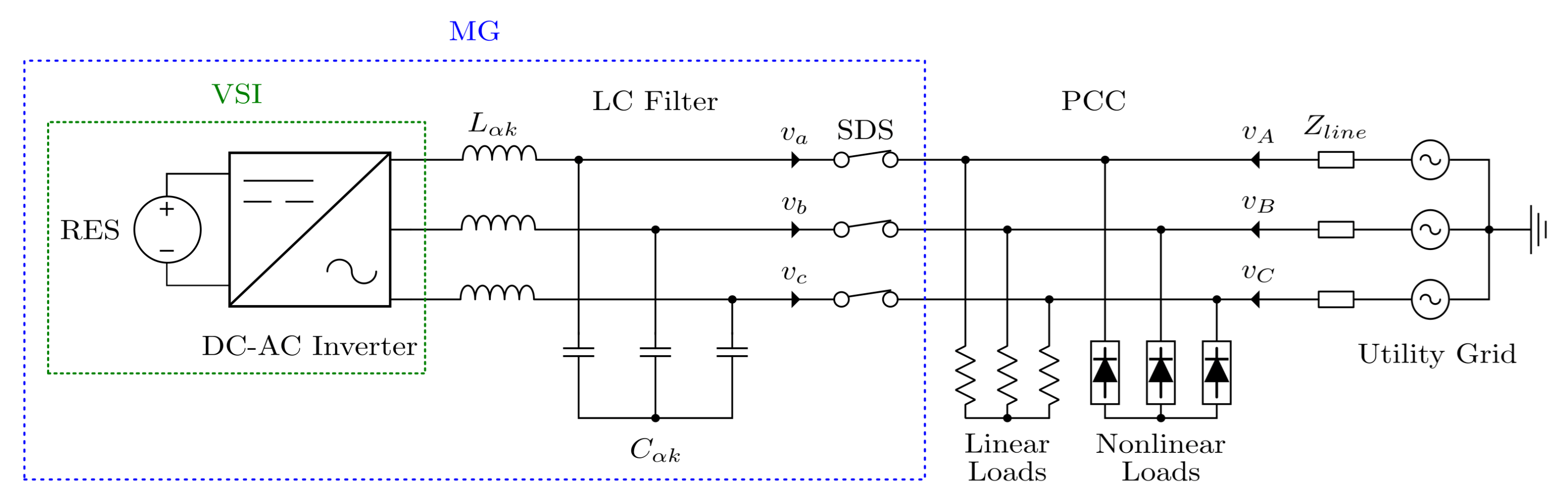
2.2. Microgrid Model

A microgrid (MG) is a scheme used for generating, distributing, and regulating power flow into an electrical grid. Such a scheme can operate in two configurations: grid-tied and isolated mode. These lead to a characterization of MGs as autonomous or decentralized systems, respectively. In the first case, unbalanced voltages and currents are generated by unbalanced loads and issues within the utility grid, degrading the energy quality index [33]. Note that any anomaly in the electrical grid directly affects the MG performance. For the isolated mode, the MG is disconnected from the utility grid and operates as an autonomous system. Thence, the disequilibrium in voltages and currents is caused by unbalanced loads.

An MG allows users to integrate renewable energy sources; so, representing a sustainable, efficient, and safe alternative for supplying energy. Even though there can be different kinds of MGs, for this work, we consider the one depicted in Figure 2.

In electrical terms, the MG contains a Renewable Energy Source (RES), a three-phase converter, a filter (in this case, made up to a capacitor and an inductor), and a Static Disconnect Switch (SDS). This set of elements feed linear and nonlinear loads connected at the PCC between the MG and the utility grid. The latter is constituted by a three-phase voltage source and the respective coupling impedance.

Mathematically speaking, the RES–Converter duo can be modeled as an ideal voltage source. The reason is that the IBC extracts energy directly from photovoltaic cells. Thus, there are no mechanical components generating inertia, as is the case with wind turbines and microturbines, among others [34]. Similarly, we assume a 99% efficiency for the three-phase converter [35]. Bear in mind that in the MG model, the IBC is interpreted as a RES.

The Park transform (PT) is a strategy that can be used for simplifying the electrical three-phase model into the Direct-Quadrature-Zero ($dq0$) domain. In this way, the MG model is decoupled, facilitating the description of its behavior [36]. The mapping process of the PT begins by considering that passive elements within the LC filter have the same value for each phase. Therefore, their three-phase framework representation is given by

$$\begin{array}{c}\hfill {\mathit{L}}_{\alpha k}=l_k{I}_3,\\ \hfill {\mathit{C}}_{\alpha k}=c_k{I}_3,\end{array}$$

(8)

where $I_3$ is the identity matrix of order 3, and $l_k$ and $c_k$ are the scalar values for the inductor and capacitor bank by phase, respectively. Afterward, the reference system is changed from $abc$ to $dq$, sans the homopolar component, for (8) using the following current–tension relations:

$$\begin{array}{c}\hfill v_{abc}^{{\mathit{L}}_{\alpha k}}={\mathit{L}}_{\alpha k}\frac{d}{dt}{i}_{abc}^{{\mathit{L}}_{\alpha k}},\\ \hfill i_{abc}^{{\mathit{C}}_{\alpha k}}={\mathit{C}}_{\alpha k}\frac{d}{dt}{v}_{abc}^{{\mathit{C}}_{\alpha k}}.\end{array}$$

(9)

Then, the concept behind the PT is applied to (9), resulting in

$$\begin{array}{cc}\hfill v_{dq}^{{\mathit{L}}_{\alpha k}}& =T_p\left(\theta \right){\mathit{L}}_{\alpha k}\frac{d}{dt}\left(T_p{\left(\theta \right)}^{-1}{i}_{dq}^{{\mathit{L}}_{\alpha k}}\right),\hfill \end{array}$$

(10)

$$\begin{array}{cc}\hfill i_{dq}^{{\mathit{C}}_{\alpha k}}& =T_p\left(\theta \right){\mathit{C}}_{\alpha k}\frac{d}{dt}\left(T_p{\left(\theta \right)}^{-1}{v}_{dq}^{{\mathit{C}}_{\alpha k}}\right),\hfill \end{array}$$

(11)

where $T_p\left(\theta \right)$ is the PT operator, which is a function of the axes angular-speed $\theta$; that in turn, is defined such as $\theta =\omega t$. The $dq$ representation of passive elements is achieved via the chain rule when plugging in (10) and (11), which yields

$$\begin{array}{cc}\hfill v_d^{l_k}& =-\omega l_k{i}_q^{l_k}+l_k\frac{d}{dt}{i}_d^{l_k},\hfill \end{array}$$

(12)

$$\begin{array}{cc}\hfill v_q^{l_k}& =\omega l_k{i}_d^{l_k}+l_k\frac{d}{dt}{i}_q^{l_k},\hfill \end{array}$$

(13)

$$\begin{array}{cc}\hfill i_d^{c_k}& =-\omega c_k{v}_q^{c_k}+c_k\frac{d}{dt}{v}_d^{c_k},\hfill \end{array}$$

(14)

$$\begin{array}{cc}\hfill i_q^{c_k}& =\omega c_k{v}_d^{c_k}+c_k\frac{d}{dt}{v}_q^{c_k}\hfill \end{array}$$

(15)

In this sense, the PT can be applied to the Thevenin equivalent of the MG structure using trivial circuit analysis theory [37]. Moreover, the MG dynamic in state-space is represented by

$$\begin{array}{c}\hfill \begin{array}{cc}\hfill \frac{d}{dt}\left(\begin{array}{c}{i}_d^L\\ i_q^L\\ v_d^C\\ v_q^C\end{array}\right)& =\left(\begin{array}{cccc}0& \omega & -\frac{1}{L}& 0\\ -\omega & 0& 0& -\frac{1}{L}\\ \frac{1}{C}& 0& 0& \omega \\ 0& \frac{1}{C}& -\omega & 0\end{array}\right)\left(\begin{array}{c}{i}_d^L\\ i_q^L\\ v_d^C\\ v_q^C\end{array}\right)\hfill \\ \hfill & +\left(\begin{array}{cccc}\frac{1}{L}& 0& 0& 0\\ 0& \frac{1}{L}& 0& 0\\ 0& 0& -\frac{1}{C}& 0\\ 0& 0& 0& -\frac{1}{C}\end{array}\right)\left(\begin{array}{c}{u}_d\\ u_q\\ i_{s_d}\\ i_{s_q}\end{array}\right),\hfill \\ \hfill y& =\left(\begin{array}{cccc}0& 0& 1& 1\end{array}\right)\left(\begin{array}{c}{i}_d^L\\ i_q^L\\ v_d^C\\ v_q^C\end{array}\right).\hfill \end{array}\end{array}$$

(16)

Taking advantage of the PT properties [38], the system shown in (16) can be decoupled into the $dq$ reference frame such as

$$\begin{array}{cc}\hfill \frac{d}{dt}\left(\begin{array}{c}{i}_d^L\\ v_d^C\end{array}\right)=& \stackrel{\mathit{A}}{\overbrace{\left(\begin{array}{cc}0& -\frac{1}{L}\\ \frac{1}{C}& 0\end{array}\right)}}\left(\begin{array}{c}{i}_d^L\\ v_d^C\end{array}\right)+\stackrel{\mathit{B}}{\overbrace{\left(\begin{array}{c}\frac{1}{L}\\ 0\end{array}\right)}}{u}_d+\overrightarrow{g}\left(x\right),\hfill \\ \hfill & y=\stackrel{\overrightarrow{C}}{\overbrace{\left(\begin{array}{cc}0& 1\end{array}\right)}}\left(\begin{array}{c}{i}_d^L\\ v_d^C\end{array}\right),\hfill \end{array}$$

(17)

$$\begin{array}{cc}\hfill \frac{d}{dt}\left(\begin{array}{c}{i}_q^L\\ v_q^C\end{array}\right)=& \stackrel{\mathit{A}}{\overbrace{\left(\begin{array}{cc}0& -\frac{1}{L}\\ \frac{1}{C}& 0\end{array}\right)}}\left(\begin{array}{c}{i}_q^L\\ v_q^C\end{array}\right)+\stackrel{\mathit{B}}{\overbrace{\left(\begin{array}{c}\frac{1}{L}\\ 0\end{array}\right)}}{u}_q+\overrightarrow{h}\left(x\right),\hfill \\ \hfill & y=\stackrel{\overrightarrow{C}}{\overbrace{\left(\begin{array}{cc}0& 1\end{array}\right)}}\left(\begin{array}{c}{i}_q^L\\ v_q^C\end{array}\right),\hfill \end{array}$$

(18)

where $u_d$ [V] and $u_q$ [V] represent the $dq$ components of the voltage delivered by the IBC. Moreover, $\overrightarrow{g}\left(x\right)$ and $\overrightarrow{h}\left(x\right)$ represent the system response to perturbations modeled with (19) and (20), respectively.

$$\begin{array}{cc}\hfill \overrightarrow{g}\left(x\right)& =\left(\begin{array}{cc}\omega & 0\\ 0& \omega \end{array}\right)\left(\begin{array}{c}{i}_d^L\\ v_d^C\end{array}\right)-\left(\begin{array}{c}0\\ \frac{1}{C}\end{array}\right)i_{s_d},\hfill \end{array}$$

(19)

$$\begin{array}{cc}\hfill \overrightarrow{h}\left(x\right)& =-\left(\begin{array}{cc}\omega & 0\\ 0& \omega \end{array}\right)\left(\begin{array}{c}{i}_q^L\\ v_q^C\end{array}\right)-\left(\begin{array}{c}0\\ \frac{1}{C}\end{array}\right)i_{s_q}.\hfill \end{array}$$

(20)

Bear in mind that throughout these equations, $d{i}_d^L/dt$ [A/s], $d{i}_q^L/dt$ [A/s], $d{v}_d^C/dt$ [V/s], and $d{v}_q^C/dt$ [V/s] are related the voltages and currents of inductors ($L_{\alpha k}$ [H]) and capacitors ($C_{\alpha k}$ [F]), respectively. Likewise, $i_d^L$ [A], $i_q^L$ [A] are the inductor currents and $v_d^C$ [V], $v_q^C$ [V] are the capacitor voltages, including $i_{s_d}$ [A], $i_{s_q}$ [A] as the signals coming from the electrical grid in the $dq$ reference frame.

2.3. Metaheuristics

Metaheuristics (MHs) are procedures that may range from quite simple approaches to sophisticated ones. They have been used to assess the solution of a wide array of problems. Their use is customary nowadays because of their proven success, flexibility, and simplicity. Besides, they usually are more direct than traditional approaches that require derivatives and other rigid conditions. The current literature is prolific, with examples linked to MHs. Some of the earliest ones have been used for over 30 years and are still reasonably common [39]; for example, Genetic Algorithms [40]. Throughout these years, others have been appearing, showing interesting performances and becoming popular, e.g., Particle Swarm Optimization and Gray Wolf Optimizer. Note that natural processes commonly inspire metaheuristics, so it is customary to accompany them with a corresponding metaphor [41,42]. However, metaphors say nothing about their real procedures, as Sörensen [43] criticized. It is proper to mention the research proposed by Cruz-Duarte et al. [44], which settles the foundations for studying and somehow classifying MHs by focusing on the mathematical procedure representing such metaheuristics.

Before describing the MHs that we implement for this work, we consider it crucial to review two common concepts. The first one is the population employed by many metaheuristics in the literature [41,44]. A population $X\left(\tau \right)$ is defined as a set of N candidate solutions at iteration $\tau$ for an optimization problem given by a feasible domain $\mathfrak{X}$ and an objective function $f:\mathfrak{X}\mapsto \mathbb{R}$, which is modified in an iterative procedure, i.e., $X\left(\tau \right)=\{{\overrightarrow{x}}_1\left(\tau \right),\cdots ,{\overrightarrow{x}}_N\left(\tau \right)\}$. Then, ${\overrightarrow{x}}_n\left(\tau \right)\in X\left(\tau \right)$ denotes the position of the nth individual (or agent). In this work, we consider a continuous problem domain, so $\mathfrak{X}\subseteq {\mathbb{R}}^D$, where D stands for the number of dimensions. Plus, for the sake of simplicity, we regard a parallelepipedical feasible region given by

$$\mathfrak{X}=\left\{\forall \overrightarrow{x}\in {\mathbb{R}}^D:\left(\exists {\overrightarrow{x}}_l,{\overrightarrow{x}}_u\in {\mathbb{R}}^D\right)[{\overrightarrow{x}}_l⪯\overrightarrow{x}⪯{\overrightarrow{x}}_u]\right\}$$

(21)

as ${\overrightarrow{x}}_l$ and ${\overrightarrow{x}}_u$ are the lower and upper limits, respectively.

The second concept, always present in all metaheuristics, is the best position ${\overrightarrow{x}}_{\ast }$. To define it, we may consider an arbitrary set of candidate positions Z, which can be designated as, e.g., the entire population $Z=X$, the nth neighborhood $Z=Y_n$, and the historical evolution of the nth candidate $Z=\{{\overrightarrow{x}}_n\left(0\right),\cdots ,{\overrightarrow{x}}_n\left(\tau \right)\}$, since $\tau$ is the current iteration. Therefore, the best position from $Z\left(t\right)$ corresponds to ${\overrightarrow{x}}_{\ast }\in Z$, i.e., ${\overrightarrow{x}}_{\ast }=arginf\left\{f\left(Z\right)\right\}$ for a minimization problem. Bearing this in mind, we now comment on the methods used for this work.

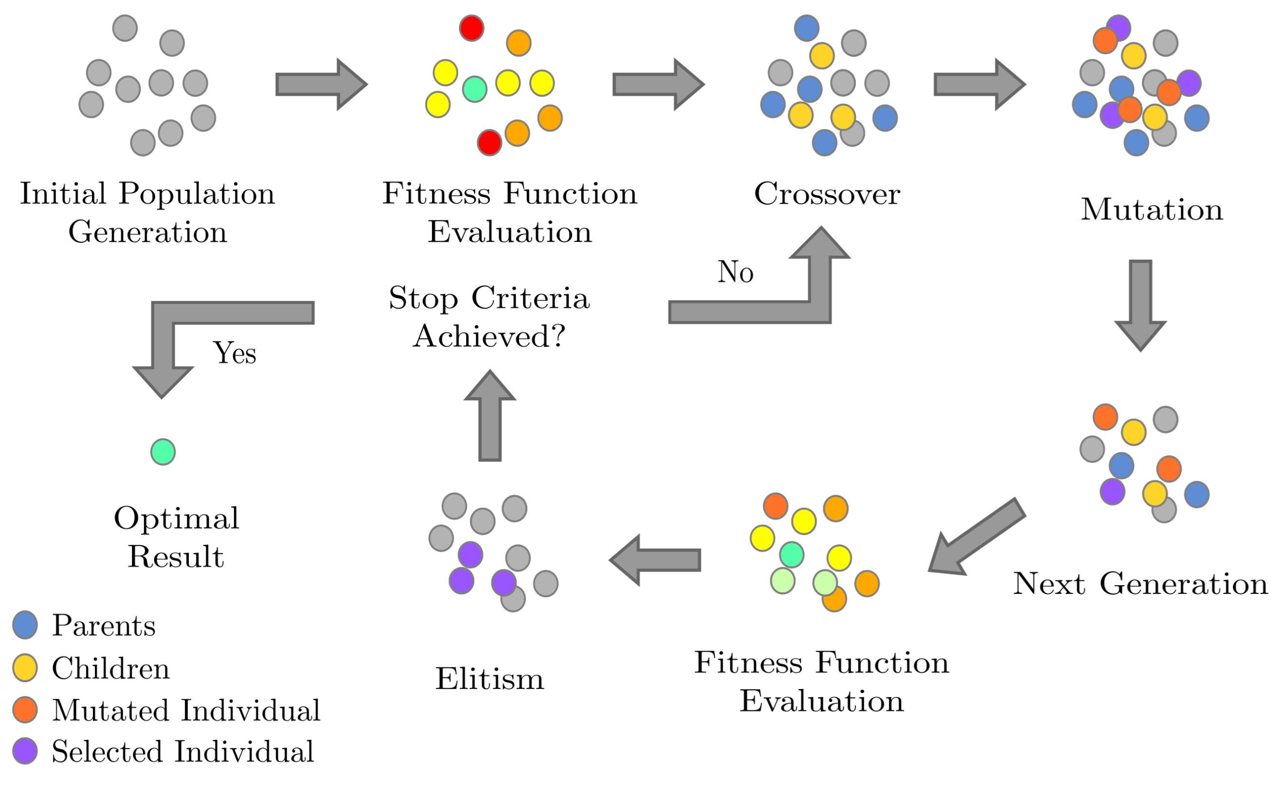
2.3.1. Genetic Algorithms

Genetic Algorithms (GAs) seek to replicate the natural selection process and so their search agents are given by chromosomes, or genotypes, which can be represented as strings of either binary or real-valued numbers [45]. GA is a population-based methodology that, throughout an iterative process, strives to refine (evolve) such a population. This evolution is achieved by using diverse genetic operators that alter chromosomes, aiming to improve their quality measure [46], usually referred to as fitness. Commonplace genetic operators include crossover, mutation, and selection. The first one combines the information of the current population, while the second introduces genetic diversity by randomly modifying some of the individuals. The final operator (also known as elitism) decides which individuals will have the opportunity to provide genetic material for the next generations. Their relationships and an overview of the whole procedure are illustrated in Figure 3.

As this work deals with a continuous problem domain, the crossover and mutation operators are based on the standard versions used for real-valued chromosomes. Then, for crossover, the arithmetic approach is employed, as described below,

$${\overrightarrow{x}}_c={\alpha }_c\left({\overrightarrow{r}}_u\odot {\overrightarrow{x}}_{p,1}+(1-{\overrightarrow{r}}_u)\odot {\overrightarrow{x}}_{p,2}\right),$$

(22)

where ${\overrightarrow{x}}_c$ is the position of a child, and ${\overrightarrow{x}}_{p,1}$ and ${\overrightarrow{x}}_{p,2}$ are two parent chromosomes from the current population. These parents are chosen via a pairing scheme, for example, random, tournament, and roulette wheel. We utilize a random pairing scheme in this GA implementation. Moreover, ${\overrightarrow{r}}_u\ni r_k\sim \mathcal{U}(0,1)$ is a vector of i.i.d. random numbers with uniform distribution, ${\alpha }_c\in {\mathbb{R}}_{+}$ is a controlling factor, and ⊙ is the Hadamard–Schur’s product. Plus, this crossover procedure must be carried out for as many children are required to be considered for the next generation.

For mutation, we allow individuals to change within a range given by ${\overrightarrow{x}}_l$ and ${\overrightarrow{x}}_u$, cf. (21). Therefore, we implemented

$${\overrightarrow{x}}_n^{\prime }=(1-{\alpha }_m){\overrightarrow{x}}_n+{\alpha }_m{\overrightarrow{r}}_u$$

(23)

as ${\overrightarrow{x}}_n^{\prime }$ is a mutant version of the individual (chromosome) ${\overrightarrow{x}}_n$, ${\overrightarrow{r}}_u$ is a vector of i.i.d. random numbers such as ${\overrightarrow{r}}_u\ni r_d\sim \mathcal{U}(x_{l,d},x_{u,d})$, $\forall d\in \{1,\cdots ,D\}$, and ${\alpha }_m\in [0,1]$ is the percentage of information to mutate for each element in the chromosome. After applying this procedure, GA generally has multiple ways to decide if the originals or mutants are preserved. The most common one is the well-known Greedy criterion, which consists of keeping the best version for each individual according to their fitness value. We employ this approach in this GA implementation.

The last genetic operator, the selection, is carried out through a random sampling process with uniform distribution. This decision is based on preliminary empirical evidence on the performance of the GA for this particular problem. Bear in mind that this operator seeks to preserve the population size, then some ‘newborns’, ‘mutants’, and ‘parents’ are neglected for the new generation. Besides, GA relies on elitism to keep some of the best individuals of the population, so their promising genetic material is not compromised.

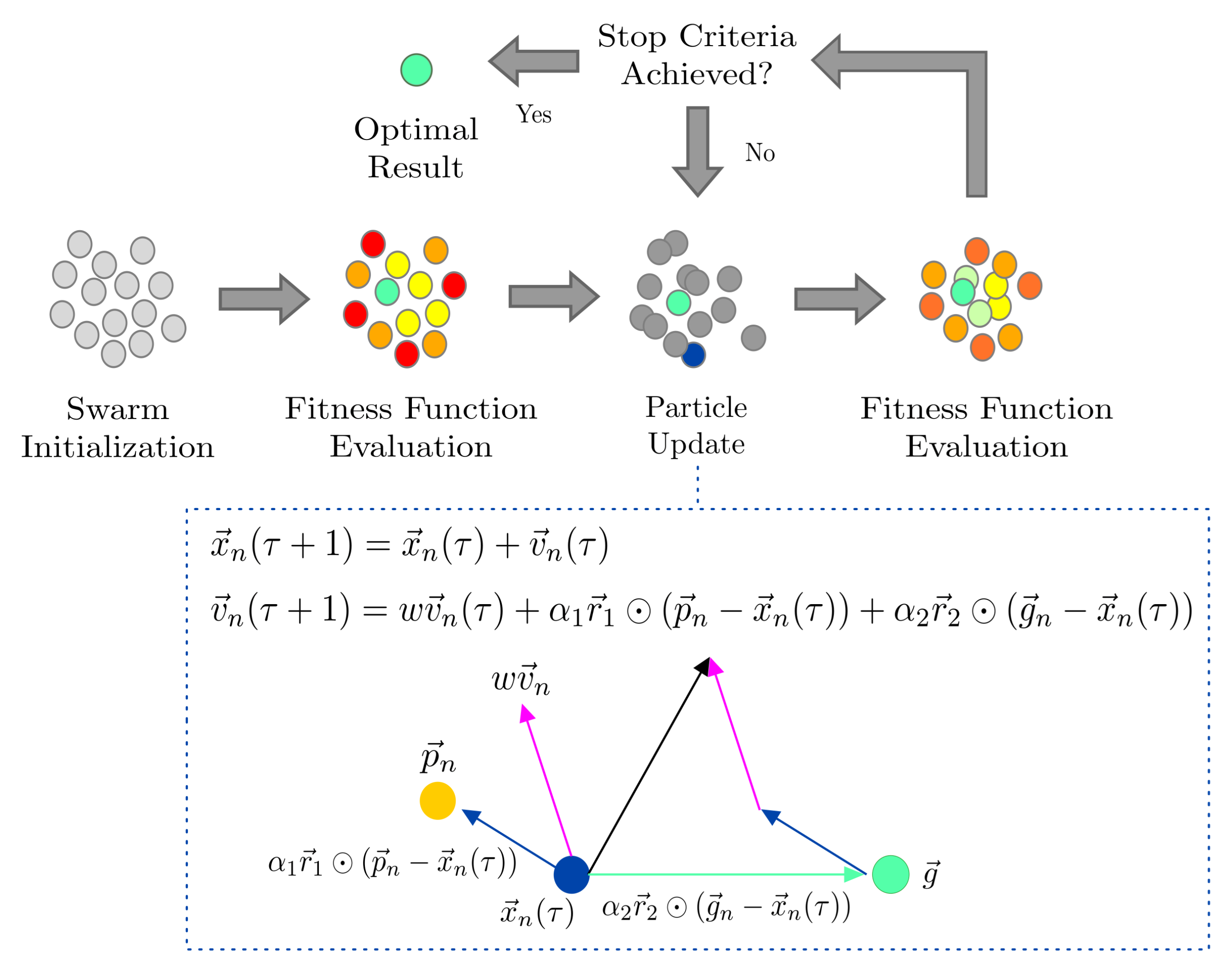
2.3.2. Particle Swarm Optimization

Particle Swarm Optimization (PSO) is inspired by the collective behavior of birds and fish [47]. Therefore, as with the previous approach, it considers a collection of search agents. In this case, each agent is called a particle, and their collection is said to form “a swarm”. Moreover, each agent has a position ${\overrightarrow{x}}_n$ and a velocity ${\overrightarrow{v}}_n$, where the former provides candidate solutions to a given problem.

During the iterative process of PSO, the particles are constantly moving and exploring the search space via a simple kinematic dynamic. It leads to some elements worthy of highlighting. For starters, the best position ${\overrightarrow{p}}_n$ that a particle n has found must be preserved and updated accordingly; this is known as the personal best. Consequently, one of these positions also represents the best position found by the whole swarm, $\overrightarrow{g}$; this is known as the global best. Furthermore, in a given iteration $\tau$, the current position of the particle may differ from its personal best, as they are always moving. Therefore, the movement of a particle is determined by several factors [48], including the current parameters and the best solutions. These elements are liaised through

$${\overrightarrow{x}}_n(\tau +1)={\overrightarrow{x}}_n\left(\tau \right)+{\overrightarrow{v}}_n\left(\tau \right),$$

(24)

and

$$\begin{array}{cc}\hfill {\overrightarrow{v}}_n(\tau +1)=w{\overrightarrow{v}}_n\left(\tau \right)& +{\alpha }_1{\overrightarrow{r}}_1\odot ({\overrightarrow{p}}_n-{\overrightarrow{x}}_n\left(\tau \right))+{\alpha }_2{\overrightarrow{r}}_2\odot (\overrightarrow{g}-{\overrightarrow{x}}_n\left(\tau \right)).\hfill \end{array}$$

(25)

Equation (24) represents the actual movement of the n^th particle and requires the current position and velocity of the particle, ${\overrightarrow{x}}_n\left(\tau \right)$ and ${\overrightarrow{v}}_n\left(\tau \right)$, respectively, whereas (25) updates the velocity of the nth particle. For such a dynamic, it is required the current position of the nth particle; the personal and global best positions, ${\overrightarrow{p}}_n$ and $\overrightarrow{g}$, respectively; the inertia factor $w\in [0,1[$; the self-confidence coefficient ${\alpha }_1\in {\mathbb{R}}_{+}$; and the swarm confidence coefficient ${\alpha }_2\in {\mathbb{R}}_{+}$. These formulae also employ a couple of vectors with i.i.d. random elements with uniform distribution, ${\overrightarrow{r}}_i\ni r_{i,k}\sim \mathcal{U}(0,1)\forall i=\{1,2\}$. Bear in mind that w is included as a control mechanism for avoiding the swarm explosion [49]. In Figure 4, we present an illustrative example of how the PSO procedure is employed for solving a problem.

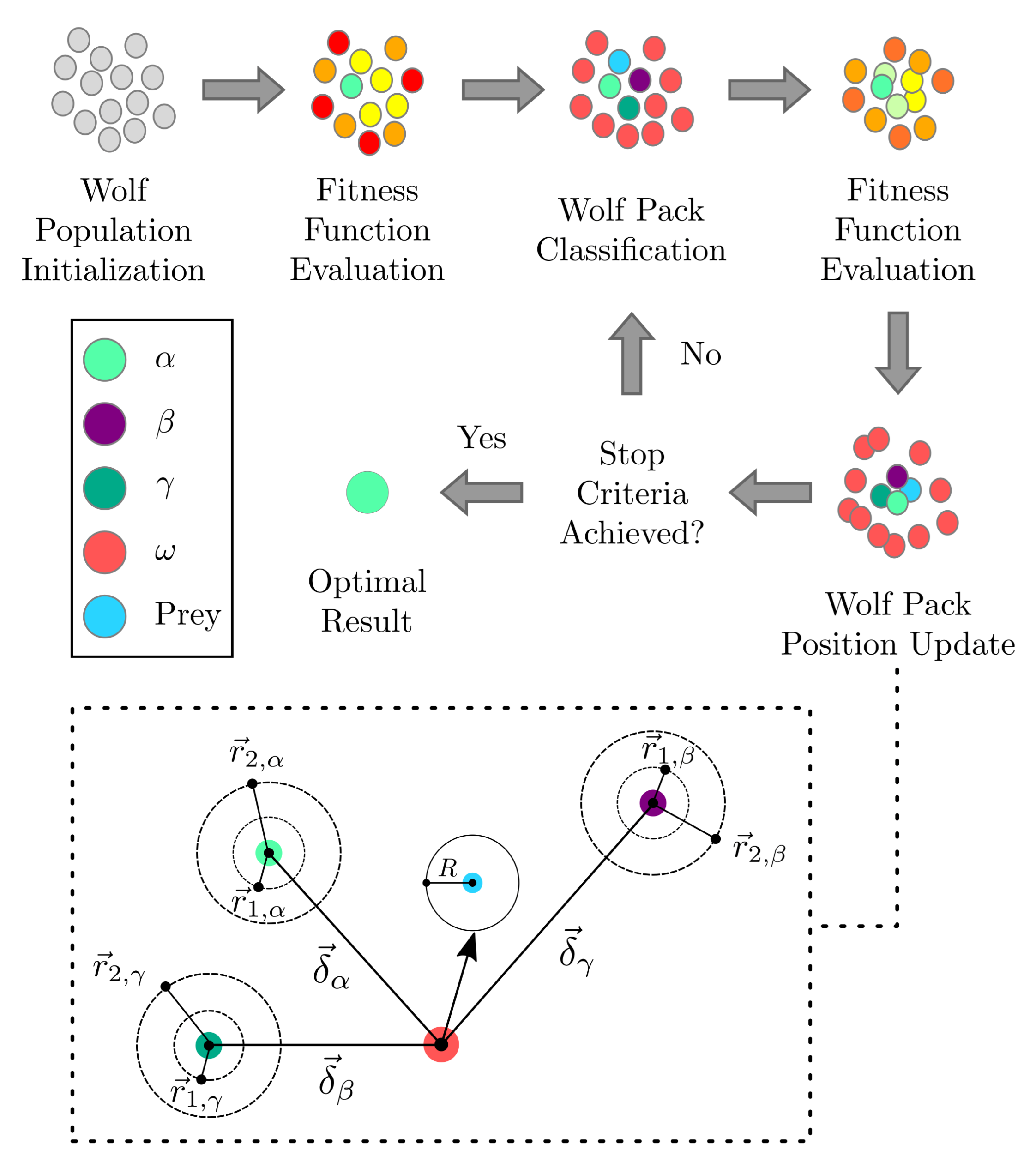
2.3.3. Gray Wolf Optimizer

Gray Wolf Optimizer (GWO) seeks to mimic the hunting behavior of grey wolves by considering a group of search agents with a strict hierarchy [50], i.e., $\alpha$ individuals sit at the top, followed by $\beta$, and $\gamma$ wolves. The remaining individuals are regarded to be of the $\omega$ class. Now, the “hunting process of wolves” gives place to the position update for each individual in the population, mathematically described by

$${\overrightarrow{x}}_n(\tau +1)=\frac{1}{3}\sum _i\left({\overrightarrow{x}}_i-2{\overrightarrow{r}}_{1,i}\odot \overrightarrow{\delta }\left(\tau \right)\odot \overrightarrow{a}\left(\tau \right)\right),\forall i\in \{\alpha ,\beta ,\gamma \},$$

(26)

with

$${\overrightarrow{\delta }}_i\left(\tau \right)={\left|2{\overrightarrow{r}}_{2,i}\odot {\overrightarrow{x}}_i-{\overrightarrow{x}}_n\left(\tau \right)\right|}_{\odot },\forall i\in \{\alpha ,\beta ,\gamma \},$$

(27)

as $\tau$ is the current iteration, ${\overrightarrow{x}}_n\left(\tau \right)$ stands the current position of the nth individual, ${\overrightarrow{x}}_i\left(\tau \right)$ represents the position of an elite wolf (i.e., $\alpha$, $\beta$, and $\gamma$), and ${\overrightarrow{r}}_{1,i}\ni r_{1,i,k}\sim \mathcal{U}(-1,1)$ and ${\overrightarrow{r}}_{2,i}\ni r_{2,i,k}\sim \mathcal{U}(0,1)$ are vectors of i.i.d. random elements. Consider that $|\overrightarrow{y}{|}_{\odot }=\left(\right|y_1|,\cdots ,|y_D{\left|\right)}^{⊺}$, with $\overrightarrow{y}\in {\mathbb{R}}^D$ as a dummy vector, is the element-wise version of the absolute value operator for vectors. Moreover, $\overrightarrow{a}\left(\tau \right)$ is a vector of components linearly decreasing from 2 to 0 w.r.t. iterations. In this work, we use the formula given by Mirjalili et al. [50], such as

$$\overrightarrow{a}\left(\tau \right)=2\left(1-\frac{\tau }{{\tau }_{\max }}\right)\overrightarrow{1},\mathrm{with}\overrightarrow{1}={(1,\cdots ,1)}^{⊺}\in {\mathbb{R}}^D,$$

(28)

where ${\tau }_{\max }$ is the maximal number of iterations.

Figure 5 provides an overview of the GWO approach and details how each search agent moves throughout the search space, depending on the location of the $\alpha$, $\beta$, and $\delta$ individuals.

2.4. Energy Quality

The energy quality index is a measurement of how ideal an electrical signal is. This index is determined by the voltage supplied and the operating frequency, and it evaluates whether the former is within an established range. Simultaneously, the latter must be a constant, close to a nominal value, and describe a sinusoid. This concept is affected by the phenomena that distort the waveform, such as the magnitude and phase of power signals measured at the Point of Common Coupling (PCC).

For this work, we assume that these unbalanced loads are given by a voltage with a magnitude provided by the ratio between negative and positive sequence percentages. This term is well-known as the Voltage Unbalance Factor (VUF), which is determined as follows:

$$\mathrm{VUF}=\frac{|V_{\mathrm{seq}(-)}|}{|V_{\mathrm{seq}(+)}|}\times 100\%,$$

(29)

where $V_{\sec (-)}$ and $V_{\sec (+)}$ are the negative and positive sequence components, respectively. The standard IEEE 1159–2019 recommends that the voltage imbalance (sometimes called unbalance) of a typical three-phase system must remain below 5% [6]. Another element degrading the power quality is the connection of nonlinear devices at the PCC. This is because these devices generate harmonic content that can deteriorate the MG components and the performance of the utility grid. There are some methods to attenuate the levels of this harmonic distortion, but they are often impractical and challenging to implement [51]. Moreover, the harmonic spectrum of voltage signals measured at the PCC is determined through the Total Harmonic Distortion (THD). THD is then defined by the standard IEC 61000-2-2 as the ratio between the root-sum-square of all harmonic magnitudes (excluding the fundamental) and the magnitude of the fundamental frequency [7]. When the THD index is applied to voltage signals, say ${\mathrm{THD}}_V$, it is assessed such as

$${\mathrm{THD}}_V=\frac{1}{V_1}\sqrt{\sum _{k=1}^N{V}_{2k+1}^2},$$

(30)

as $V_1$ [V] is the voltage signal corresponding to the fundamental frequency, and $V_{2k+1}$ [V] is the voltage of the harmonic $2k+1$, $\forall k=1,\cdots ,N$.

At the low-voltage distribution level, the allowed limit for the ${\mathrm{THD}}_V$ is also 5%. Thus, the ${\mathrm{THD}}_V$ in each phase of the MG is measured following this bound. Conversely, it is worth commenting that the THD index for the current is considered as a known factor for the nonlinear load connected at the PCC.

3. Our Proposed Approach

In this section, we detail our proposed approach based on the significant concepts reviewed above.

3.1. IBC Controller Optimization

An analysis of the state-space models shown in (7) reveals that the Interleaved Boost Converter (IBC) exhibits an oscillatory response to a step input. At the same time, the Microgrid (MG) provides a critically damped response. Therefore, in this work, we use the state-feedback approach [52] shown in Figure 6 when designing the controllers. This state-feedback is expressed as given,

$$\begin{array}{cc}\hfill & \overrightarrow{u}\left(t\right)=\overrightarrow{r}\left(t\right)-\mathit{K}\overrightarrow{x}\left(t\right),\hfill \\ \hfill & \dot{\overrightarrow{x}}\left(t\right)=(\mathit{A}-\mathit{B}\mathit{K})\overrightarrow{x}\left(t\right)+\mathit{B}\overrightarrow{r}\left(t\right),\hfill \end{array}$$

(31)

where $\mathit{A}$, $\mathit{B}$, and $\mathit{C}$ are matrices of the state-space representation model for IBC and MG, as shown in (7), (17), and (18). $\mathit{K}$ is the feedback matrix for the states, which is a design parameter for the LQR algorithm that seeks the best position for the poles of a system. From (31), one can manipulate the characteristic polynomial of the system, improving the IBC slow dynamic caused by the non-minimum phase problem. In this regard, we use the state-feedback approach to make the closed-loop system track step-type inputs while considering metrics such as settling time and overshoot. Furthermore, LQR is an algorithm that belongs to the theory of optimal control, which is concerned with operating a dynamic system at a low cost [53]. Additionally, $\overrightarrow{y}\left(t\right)$ is the system desired output, and $\overrightarrow{u}\left(t\right)$ and $\overrightarrow{r}\left(t\right)$ are the system input and reference, respectively.

Therefore, it is somewhat straightforward to notice that the controller can be optimized by solving the following minimization problem:

$$\begin{array}{cc}\hfill \underset{\mathit{Q},\mathit{R}}{min}\left\{J\right\}& =\underset{\mathit{Q},\mathit{R}}{min}{\int }_0^{\infty }\left({\overrightarrow{x}}^{⊺}\left(t^{\prime }\right)\mathit{Q}\overrightarrow{x}\left(t^{\prime }\right)+{\overrightarrow{u}}^{⊺}\left(t^{\prime }\right)\mathit{R}\overrightarrow{u}\left(t^{\prime }\right)\right)d{t}^{\prime },\hfill \\ \hfill \mathrm{s}.\mathrm{t}.& \dot{x}\left(t\right)=\mathit{A}\overrightarrow{x}\left(t\right)+\mathit{B}\overrightarrow{u}\left(t\right),\hfill \end{array}$$

(32)

where $\mathit{Q}$ and $\mathit{R}\in {\mathbb{R}}_{+}^{M\times M}$ are positive semi-definite matrices assigned arbitrarily. Bear in mind that $\mathit{Q}$ represents the penalization matrix for the system states, $\overrightarrow{x}\left(t\right)$. Conversely, $\mathit{R}$ relates to the velocity of the controller and $\overrightarrow{u}\left(t\right)$ are the system inputs. In this case, $\mathit{Q}$ and $\mathit{R}$ are used to calculate optimal values for $\mathit{K}$.

From this problem definition, the updated input and state vector can be obtained as shown,

$$\begin{array}{cc}\hfill & \overrightarrow{u}\left(t\right)=-\mathit{K}\overrightarrow{x}\left(t\right),\hfill \end{array}$$

(33)

$$\begin{array}{cc}\hfill & \mathit{K}={\mathit{R}}^{-1}{\mathit{B}}^{⊺}\mathit{S},\hfill \end{array}$$

(34)

as $\mathit{S}$ is achieved by solving the Riccati equation, given by

$${\mathit{A}}^{⊺}\mathit{S}+\mathit{S}\mathit{A}-\mathit{S}\mathit{B}{\mathit{R}}^{-1}{\mathit{B}}^{⊺}\mathit{S}+\mathit{Q}=\mathbf{0}.$$

(35)

Under some conditions, the LQR algorithm may fall short. For example, when faster and accurate dynamics are required. For this work, we opt to complement the LQR controller as described next. When designing the controller for the IBC, we include an integral action to obtain a controller resilient to perturbations while being robust enough to track the reference, as Figure 7 depicts.

Then, the close-loop state-space representation of the IBC becomes

$$\begin{array}{cc}\hfill \left(\begin{array}{c}\dot{\overrightarrow{x}}\left(t\right)\\ \dot{\overrightarrow{e}}\left(t\right)\end{array}\right)=\left(\begin{array}{cc}\mathit{A}& \mathbf{0}\\ -\mathbf{C}& \mathbf{0}\end{array}\right)\left(\begin{array}{c}\overrightarrow{x}\left(t\right)\\ \overrightarrow{e}\left(t\right)\end{array}\right)& +\left(\begin{array}{c}\mathit{B}\\ \mathbf{0}\end{array}\right)\overrightarrow{u}\left(t\right),\hfill \\ \hfill \overrightarrow{y}\left(t\right)=\left(\begin{array}{cc}\mathbf{C}& \mathbf{0}\end{array}\right)& \overrightarrow{x}\left(t\right)\hfill \end{array}$$

(36)

and the final state-space system with the hybrid controller, which is a Multi-Input Single- Output (MISO) system, corresponds to

$$\begin{array}{c}\hfill \begin{array}{cc}\hfill \frac{d}{dt}\left(\begin{array}{c}{i}_{L_1}\left(t\right)\\ i_{L_2}\left(t\right)\\ v_{C_1}\left(t\right)\\ e\left(t\right)\end{array}\right)& =\left(\begin{array}{cccc}0& 0& -\frac{U_1}{L_1}& 0\\ 0& 0& -\frac{U_2}{L_2}& 0\\ \frac{U_1}{C_1}& \frac{U_2}{C_1}& -\frac{1}{R{C}_1}& 0\\ 0& 0& -1& 0\end{array}\right)\left(\begin{array}{c}{i}_{L_1}\left(t\right)\\ i_{L_2}\left(t\right)\\ v_{C_1}\left(t\right)\\ e\left(t\right)\end{array}\right)\hfill \\ \hfill & +\left(\begin{array}{cc}\frac{v_s}{U_1{L}_1}& 0\\ 0& \frac{v_s}{U_2{L}_2}\\ -\frac{v_s}{R{C}_1{U}_1^2}& -\frac{v_s}{R{C}_1{U}_2^2}\\ 0& 0\end{array}\right)\left(\begin{array}{c}{U}_{d_1}\\ U_{d_2}\end{array}\right),\hfill \\ \hfill & y\left(t\right)=\left(\begin{array}{cccc}0& 0& 1& 0\end{array}\right)\left(\begin{array}{c}{i}_{L_1}\left(t\right)\\ i_{L_2}\left(t\right)\\ v_{C_1}\left(t\right)\\ e\left(t\right)\end{array}\right).\hfill \end{array}\end{array}$$

(37)

In Equation (37), the inputs are given by the duty cycle of inductors ($U_{d_1}$ and $U_{d_2}$), and the output $y\left(t\right)$ corresponds to the capacitor voltage ($v_{C_1}$). Therefore, we design one controller for each input, as shown in Figure 8, where $\overrightarrow{r}\left(t\right)$ is the IBC voltage reference and ${\overrightarrow{u}}_{1,2}\left(t\right)$ are the new inputs for the IBC states feedback. This scheme is advantageous, as we can tune each controller independently [54].

3.2. MG Controller Optimization

In the case of the microgrid (MG), we follow a similar approach. This time, however, we consider a Proportional-Integral (PI) block instead of only an integral component. This is done by striving for an accurate, fast, and robust controller. As with the previous case, the hybridizing process is shown in Figure 9, where $u_{{control}_{d,q}}$ are the new inputs for the MG states feedback, $r_{d,q}\left(t\right)$ is the MG voltage reference for d and q component, $\overrightarrow{y}\left(t\right)$ is the MG output voltage and equivalent to the states $v_d^C$ and $v_q^C$. $K_p$ and $K_i$ are the proportional and integral gains of proposed hybrid controllers, respectively. Keep in mind that for both cases, $\dot{e}$ is the controller state added to the corresponding dynamic.

Thence, the MG dynamic can be represented by

$$\begin{array}{cc}\hfill \frac{d}{dt}\left(\begin{array}{c}{i}_d^L\left(t\right)\\ v_d^C\left(t\right)\\ e\left(t\right)\end{array}\right)& =\left(\begin{array}{ccc}\frac{K_1}{L}& \frac{K_2-K_p-1}{L}& \frac{K_i}{L}\\ \frac{1}{C}& 0& 0\\ 0& -1& 0\end{array}\right)\left(\begin{array}{c}{i}_d^L\left(t\right)\\ v_d^C\left(t\right)\\ e\left(t\right)\end{array}\right)\hfill \\ \hfill & +\left(\begin{array}{c}\frac{K_p}{L}\\ 0\\ 1\end{array}\right)r_d\left(t\right),\hfill \\ \hfill y\left(t\right)& =\left(\begin{array}{ccc}0& 1& 0\end{array}\right)\left(\begin{array}{c}{i}_d^L\left(t\right)\\ v_d^C\left(t\right)\\ e\left(t\right)\end{array}\right),\hfill \end{array}$$

(38)

$$\begin{array}{cc}\hfill \frac{d}{dt}\left(\begin{array}{c}{i}_q^L\left(t\right)\\ v_q^C\left(t\right)\\ e\left(t\right)\end{array}\right)& =\left(\begin{array}{ccc}\frac{K_1}{L}& \frac{K_2-K_p-1}{L}& \frac{K_i}{L}\\ \frac{1}{C}& 0& 0\\ 0& -1& 0\end{array}\right)\left(\begin{array}{c}{i}_q^L\left(t\right)\\ v_q^C\left(t\right)\\ e\left(t\right)\end{array}\right)\hfill \\ \hfill & +\left(\begin{array}{c}\frac{K_p}{L}\\ 0\\ 1\end{array}\right)r_q\left(t\right),\hfill \\ \hfill y\left(t\right)& =\left(\begin{array}{ccc}0& 1& 0\end{array}\right)\left(\begin{array}{c}{i}_q^L\left(t\right)\\ v_q^C\left(t\right)\\ e\left(t\right)\end{array}\right).\hfill \end{array}$$

(39)

The control strategies described in (37) and (39) guarantee that such dynamic models inherit the properties of the LQR and traditional controllers. Therefore, they can provide a low-cost system operation, robust reference tracking, and steady-state error minimization. In turn, this allows for optimal energy management at the IBC-MG coupling and between the MG and the electrical grid. Notice that $\mathit{Q}$ and $\mathit{R}$ have a remarkable effect on controller performance since these matrices depend on the state number of the system and the actuator effort. Conversely, the LQR algorithm may present a poor performance for some arbitrary parameters, leading to impractical $\mathit{Q}$, $\mathit{R}$, and $\mathit{K}$ parameters that compromise controller performance. Such an issue can be addressed by implementing algorithms that render optimal elements for such matrices, e.g., metaheuristics. Additionally, one can calculate the proportional and integral gains and the LQR parameters by fusing the variables of the hybrid controller through a single fitness function that considers the system design criteria.

3.3. Fitness Function

Throughout this work, we compare the three metaheuristics presented in Section 2.3 from the perspective of controller performance. Thus, we use the overshoot, settling time, and ripple, yielded by each controller as the comparison parameters. To this end, we require the $\mathit{K}$, $\mathit{Q}$, and $\mathit{R}$ matrices, cf. (32). For the IBC, the LQR parameters are computed such as

$$\mathit{Q}=\left(\begin{array}{ccc}{q}_1& 0& 0\\ 0& q_2& 0\\ 0& 0& q_3\end{array}\right),\mathrm{and}\mathit{R}=\left(\begin{array}{cc}{r}_1& 0\\ 0& r_2\end{array}\right).$$

(40)

Similarly, the LQR parameters for the MG are given by

$$\mathit{Q}=\left(\begin{array}{cc}{q}_1& 0\\ 0& q_2\end{array}\right),\mathrm{and}\mathit{R}=r_1.$$

(41)

With this information, one can assess the performance of a given controller through

$$F=w_1\left|({MO}_{\mathrm{shoot}}-O_{\mathrm{shoot}})\right|+w_2\left|\frac{({MT}_s-T_s)}{T_s}\right|,$$

(42)

where $w_1$ and $w_2$ are values between zero and one, $w_1,w_2\in [0,1]$, for prioritizing the overshoot or the settling time, respectively. Regard that ${MO}_{\mathrm{shoot}}$ and ${MT}_{\mathrm{s}}$ are the maximum overshoot and settling time values, respectively, which are fixed by the user. Besides, $O_{\mathrm{shoot}}$ and $T_s$ are the actual values yielded by the controller, i.e., overshoot and settling time, respectively.

It is also crucial to disclose how metaheuristics represent these design variables. In the case of the IBC, there are six unknowns, i.e., three elements of $\mathit{Q}$, two of $\mathit{R}$, and the integral action $K_i$. For the MG, the number of variables is one less. The reason is that there are two unknown values for the $\mathit{Q}$ matrix, one for the $\mathit{R}$ variable and two for the PI controller ($K_i$ and $K_p$).

4. Methodology

To implement and analyze our proposed approach, we followed a two-stage methodology. Each stage focuses on a different scenario. The first one tackles the IBC as a standalone device, whereas the second merges it with an MG. In both cases, we considered the same PV array and IBC. Therefore, we assumed the parameters given in

Table 2. Parameters of the selected devices considered for this work. The PV array is arbitrarily selected with illustrative purposes, while the IBC is defined based on Habib et al. [10].

PV Array
Module	SunPower
	SPR-X20-250-BLK
Maximum Power	249.952 W
Open circuit voltage ($V_{\mathrm{oc}}$)	50.93 V
Voltage at maximum power point ($V_{\mathrm{pm}}$)	42.8 V
Temperature coefficient of $V_{\mathrm{oc}}$	−0.35602%/°C
Cells per module	72
Short-circuit current ($I_{\mathrm{sc}}$)	6.2 A
Current at maximum power point	5.84 A
Temperature coefficient of $I_{\mathrm{sc}}$	0.07%/°C
Temperature	25 °C
IBC
Resistance (R)	50 $\Omega$
Inductors ($L_1,L_2$)	5 mH
Capacitor ($C_1$)	1 mF
PV array input voltage	150 V
Switching frequency	10 kHz
Voltage set-point	300 V

for all simulations.

Additionally, we used the parameters given in

Table 3. Simulation parameters used for the metaheuristics when designing different kinds of controllers.

Parameters	IBC Controller			MG Controller
	GA	PSO	GWO	GA	PSO	GWO
Population size (N)	10	10	10	100	100	100
Max. iterations (${\tau }_{\max }$)	10	10	10	200	200	200
Elitism ratio	0.20	–	–	0.05	–	–
Crossover ratio	0.60	–	–	0.75	–	–
Mutation ratio	0.20	–	–	0.20	–	–
Inertia factor (w)	–	0.50	–	–	0.50	–
Confidence coef. (${\alpha }_1$)	–	0.50	–	–	0.50	–
Swarm coef. (${\alpha }_2$)	–	0.50	–	–	0.50	–

and repeated each experiment 30 times for statistical purposes. Note that we selected a population size of 10 for comparison purposes and following previous reports [10,17]. Moreover, although we selected the PV array with illustrative purposes, our proposal can be easily extended to other configurations. In the following lines, we provide the details about each stage.

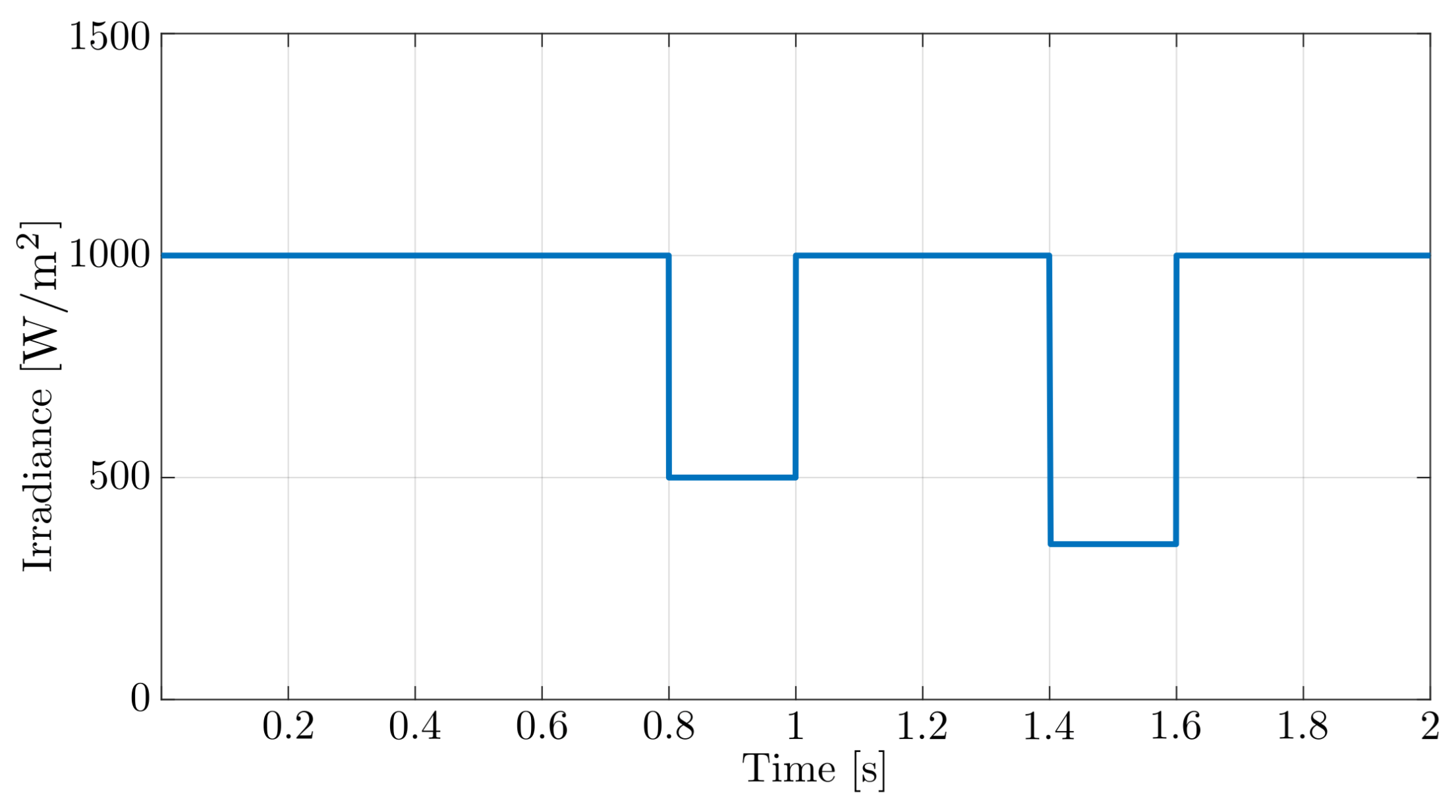
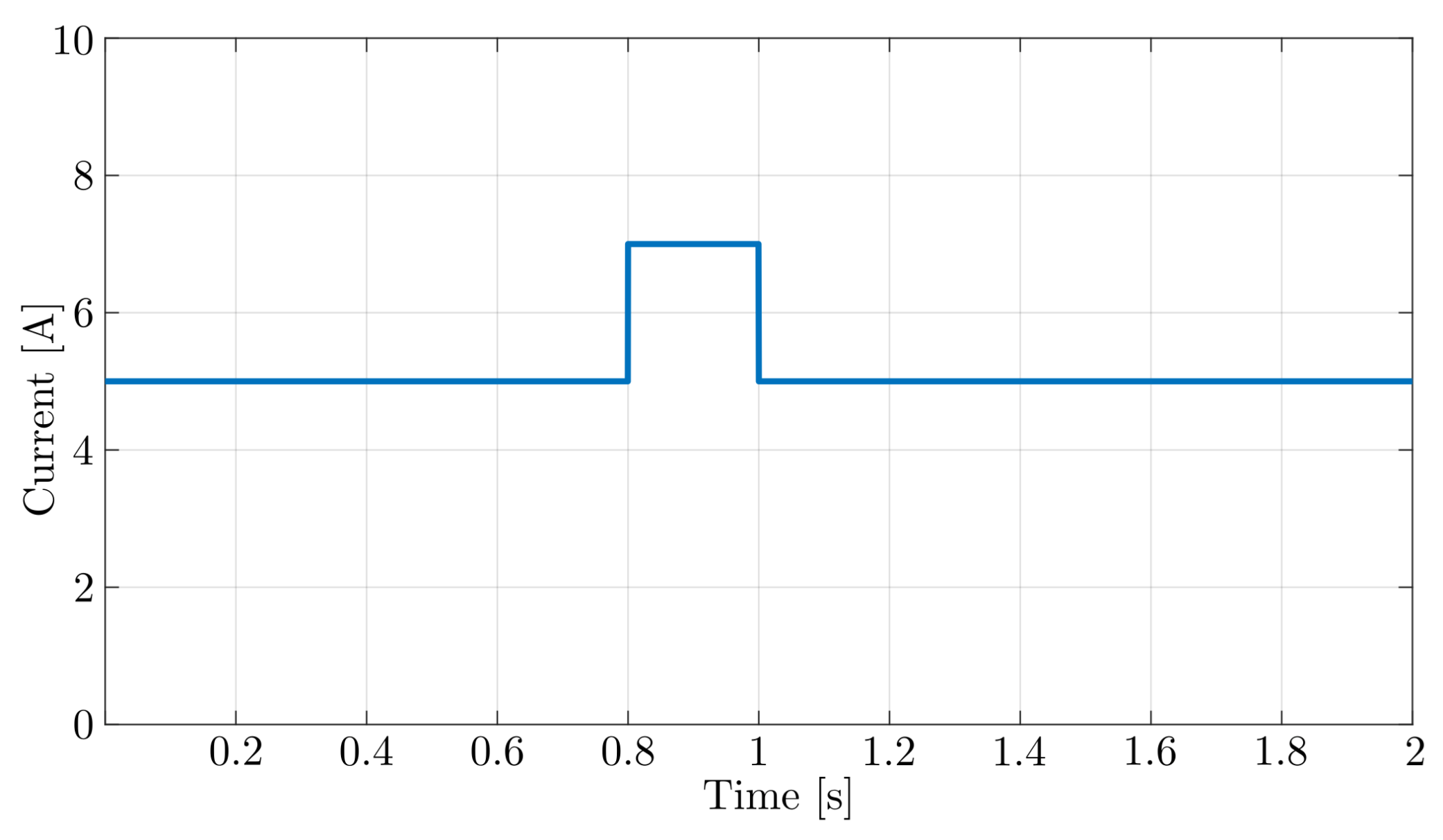
4.1. IBC Experiments

We begin by analyzing the behavior of the IBC when fed with the irradiance profile shown in Figure 10, with the task of providing the current displayed in Figure 11.

This is done to compare the performance of our proposed approach against previously published data. Therefore, we analyze the same time intervals that other authors have used before [10]. The set-point is defined to a value high enough so that it can be paired with the MG. Thus, we select a value of 300 V.

To compare the performance of the generated controllers, we analyze data for three categories: maximum overshoot, response time, and voltage ripple. We seek controllers with zero overshoot ($O_{\mathrm{shoot}}$). Nevertheless, their settling time ($T_s$) are made free, and thus they may vary w.r.t. the data reported in the literature. In this sense, we conduct a comprehensive analysis to determine the best controller configuration. Additionally, we compare the computing requirements and the performance of designing controllers with each one of the proposed metaheuristics. For this endeavor, we gather data about the integral gain of the resulting controller ($K_i$), the minimal error, the number of iterations (${\tau }_{\max }$) required by the algorithm, and the convergence time.

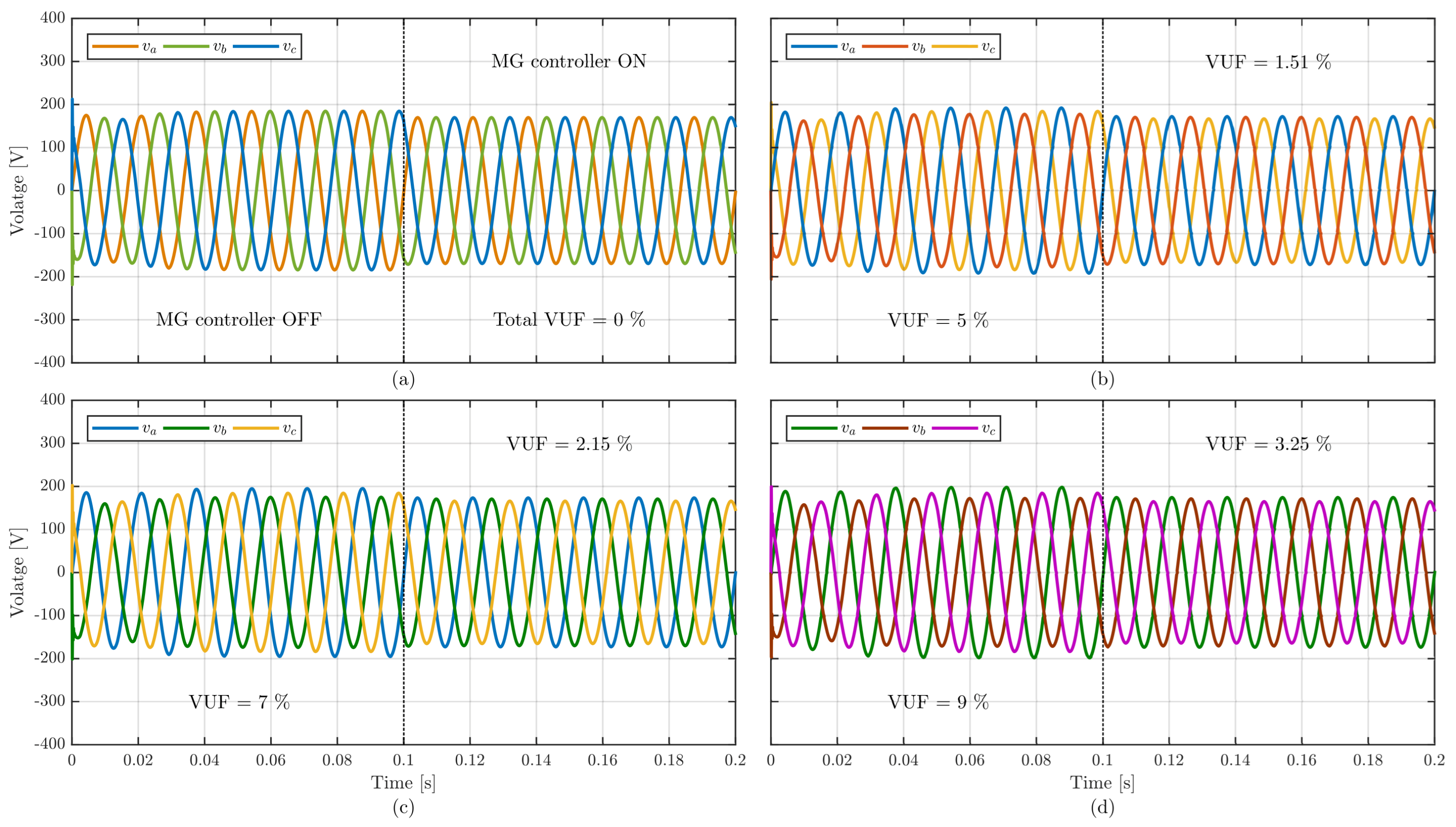
4.2. Experiments with the MG

In the second stage of our work, we verified whether our proposed approach could provide a good enough controller for an MG. Therefore, we implemented the experiment shown in Figure 12, where the parameters of the MG are shown in

Table 4. MG experiment conditions.

MG voltage	300 V
Converter switching frequency	10 kHz
Grid voltage	120 $V_{\mathrm{rms}}$
Grid frequency	60 Hz
Distribution impedance line	0.64 + 0.0377i $\Omega$
Filter inductance	12 mH
Filter capacitance	16 $\mathsf{\mu }$F
Three-phase load	20 $\Omega$
Three-phase nonlinear load capacitance	2 mF
Three-phase nonlinear load resistance	10 $\Omega$

.

In this experiment, an optimal control strategy must regulate the energy transfer between the IBC and MG so that the voltage at the PCC becomes balanced. We also developed hybrid controllers for this stage, but the fusion between PI and LQR gave them. We tuned these controllers with each one of the metaheuristics (MHs) considered in this work. Therefore, we assessed their performance in terms of the energy cost associated with the resulting controller, their error convergence, and the computational resources their tuning demands. Recall that the energy cost is directly linked to the MG voltage and the proportional gain value ($K_p$) of the controller. As the former is fixed, controllers with smaller $K_p$ lead to a lower energy cost. Thus, we sought controllers with $T_s=0.325$ ms and $O_{\mathrm{shoot}}=5$%, which were found by minimizing the cost function shown in (42).

We compared the controllers based on their overshoot, response time, and error convergence as with the previous stage. However, this time around, we also focused on the gains of the resulting controllers (i.e., $K_p$ and $K_i$). Likewise, we compared the performance of metaheuristics via their computing burden.

Our main long-term goal was to validate the MG performance when facing power quality events. Therefore, for this work, we regarded a final approach with a battery of tests based on the following conditions:

• The MG is loaded with different unbalanced voltages that come from distribution network failures, including negative sequence.
• The MG is faced with balanced nonlinear loads that exhibit harmonic contents.
• The MG is simultaneously connected to nonlinear loads and unbalanced voltages generated by the utility grid.

Note that all our experiments were run in Matlab R2021a, using a PC with a 2.60 GHz Intel Core i7-9750H CPU, 8.00 GB RAM, and Windows 10.

5. Simulation Results and Discussion

We now present the data resulting from our experiments. To make things easier for the reader, we follow the same structure from Section 4.

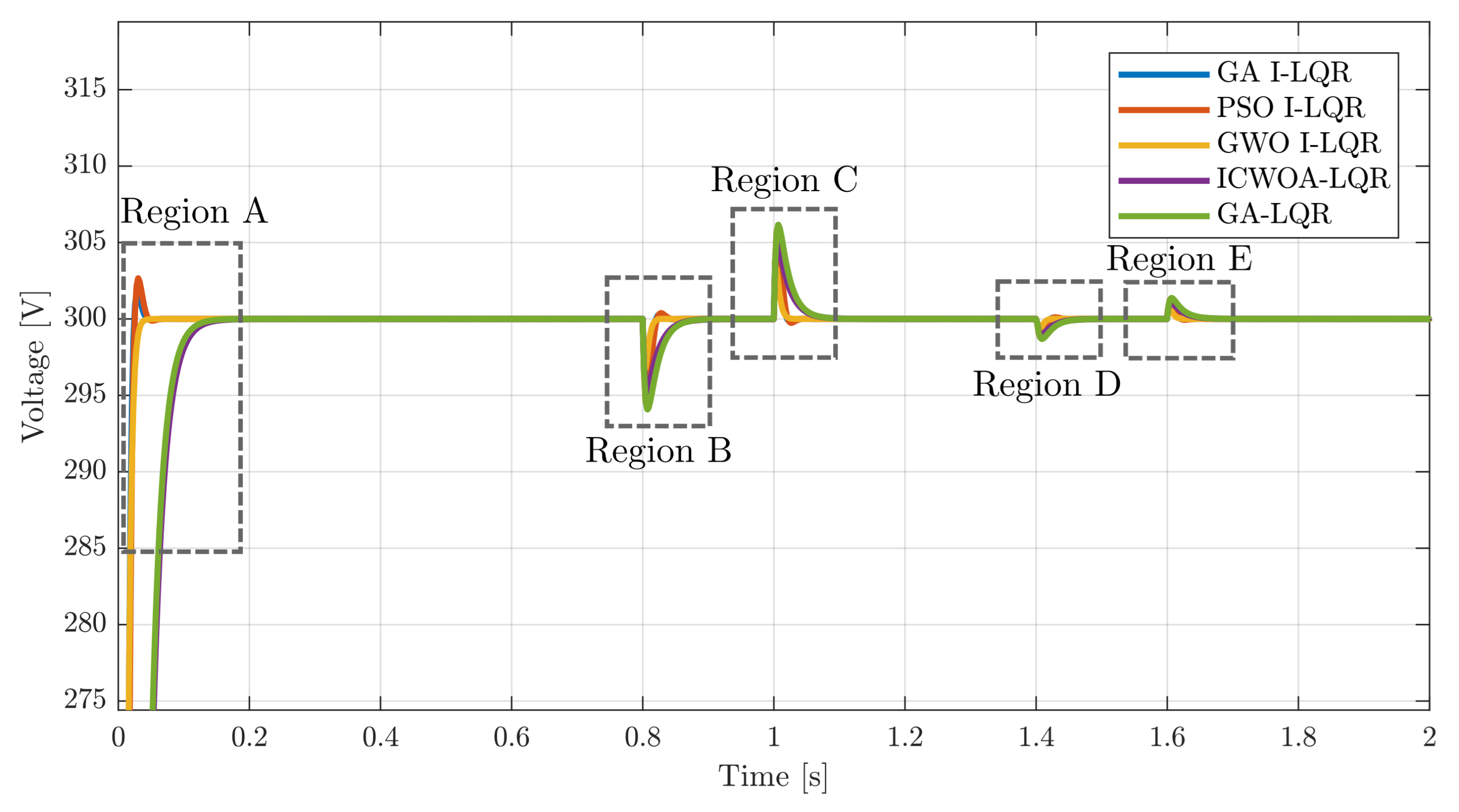
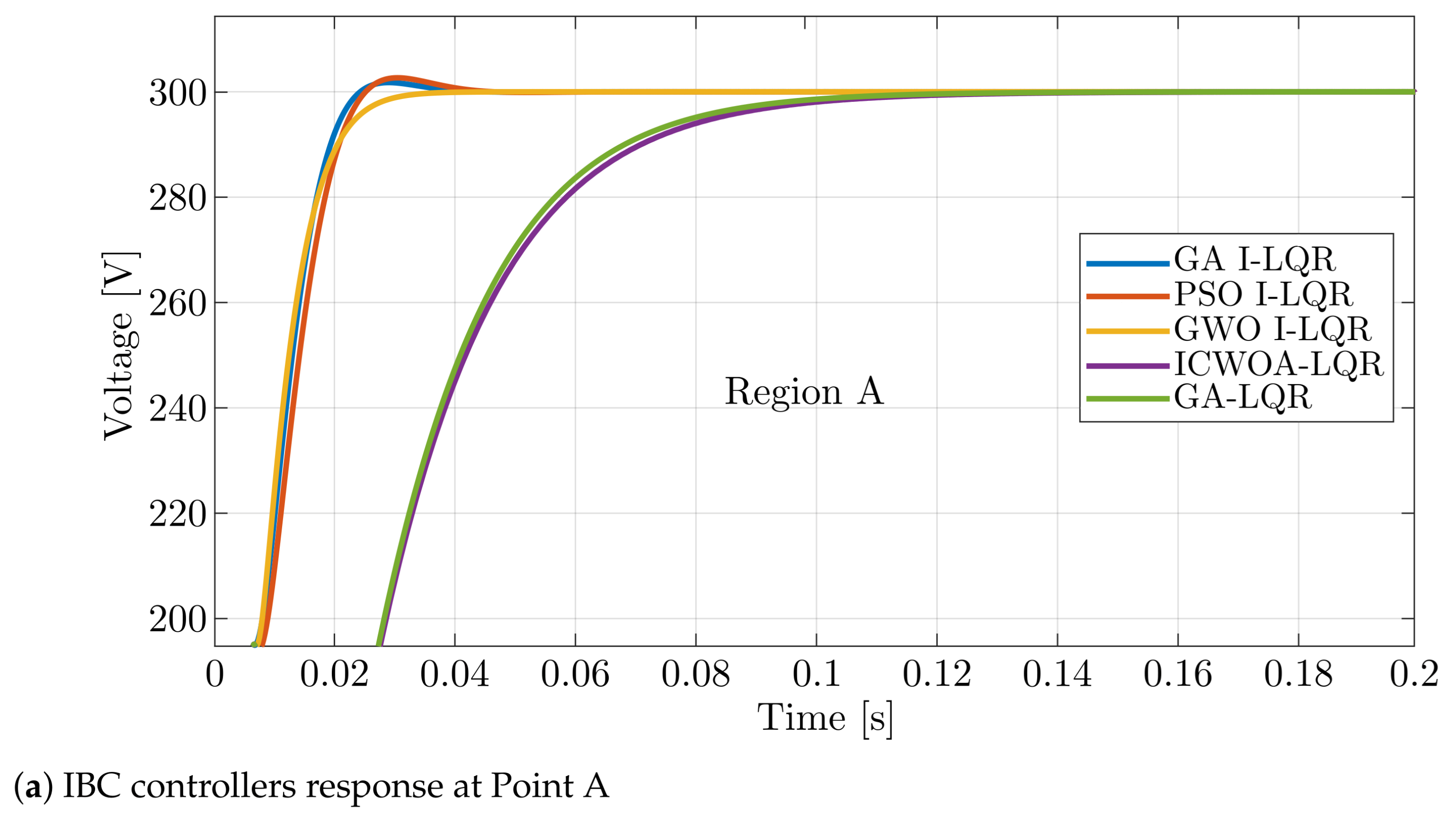
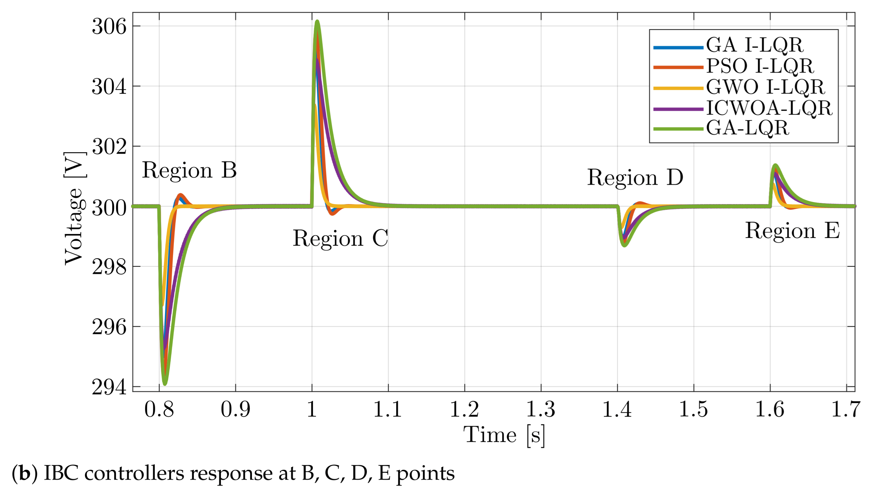
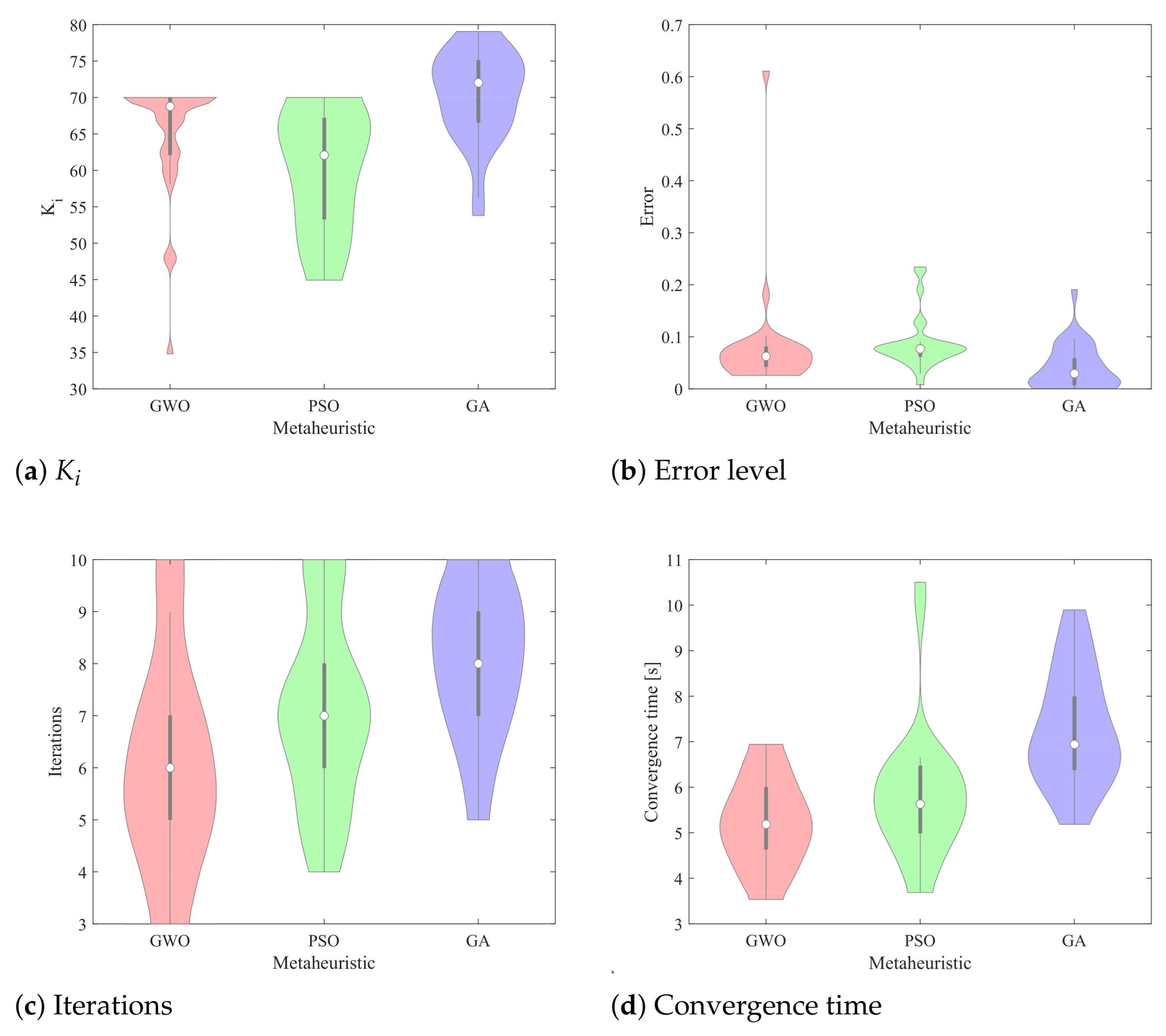
5.1. IBC Experiments

Table 5. Comparative data for the IBC controllers developed with three different metaheuristics and with previous approaches. All controllers were tuned seeking a zero overshoot and calculating the error according to (42).

Approach	Iter.	${\mathit{T}}_{\mathit{s}}$ [s]	Error	${\mathit{K}}_1$, ${\mathit{K}}_2$, ${\mathit{K}}_3$	${\mathit{K}}_{\mathit{i}}$
GA	9	0.0486	0.0486	1.5168, 0.1220, 0.5358	67.6403
PSO	8	0.0514	0.0714	4.6516, 0.3066, 1.3903	63.0782
GWO	5	0.0556	0.0644	1.8119, 0.3056, 1.2533	70
Habib et al. [10]	10	0.1410	1.0666	1.4259, 0.1127, 0.5056	27.2183
Cao et al. [17]	500	0.1781	1.4788	1.1935, 0.1165, 0.4963	25.7612
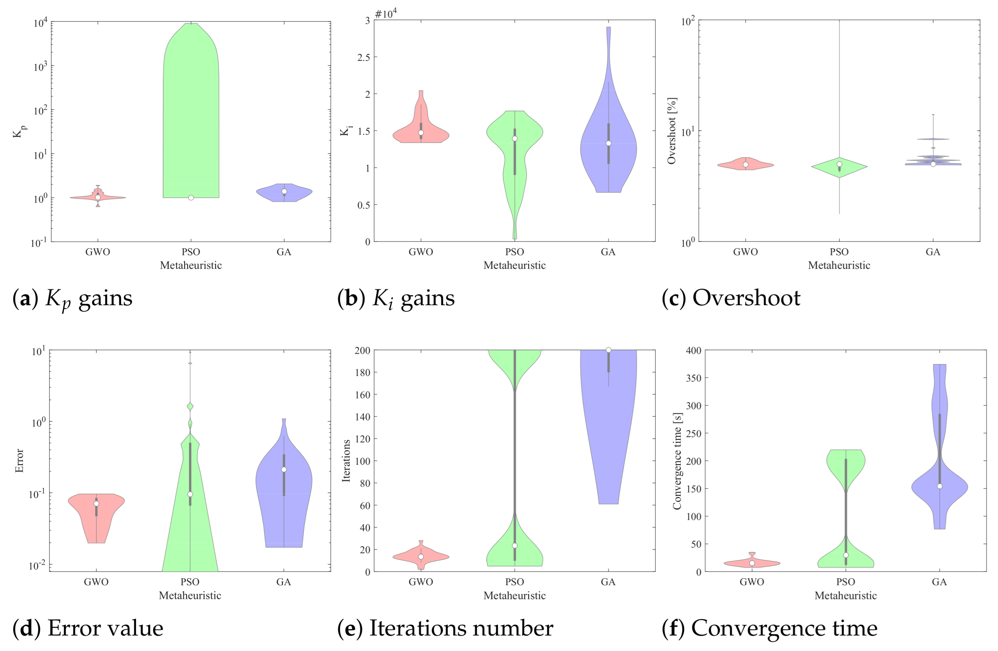
				0.1290, 1.0120, 0.5645	29.2894

presents the best controllers yielded by each one of the considered MHs and their performance, along with the data from two previous works, i.e., Habib et al. [10], Cao et al. [17]. Note that these data correspond to the response of controllers under the schemes shown in Figure 7 and Figure 8. From these results, one can evidence with ease that the controllers achieved are quicker than those from previous works. This effect is due to the values of the integral gains. Moreover, even though these values are higher than in previous works, the designs presented in Table 2 do not exceed the saturation point for the control action.

Another feature to highlight is the few iterations required by the MHs for tuning controller parameters with an excellent response ($T_s=0.045$ s, $O_{\mathrm{shoot}}=0$%). Keep in mind that Cao et al. [17] found all six values for the controller parameters, but a common approach is to simplify the search by reducing the parameters in half, as shown by Habib et al. [10]. This effect can be achieved by assuming that both controllers from Figure 8 have the same parameters. Therefore, instead of specializing each controller, we design a general one capable of handling both tasks.

Figure 13 shows the response of each controller, as well as the working regions, analyzed thoroughly in this experiment. Plus, Figure 14 details each region from Figure 13. Within the first region (Figure 14a), the controllers tuned by PSO (reddish line) and by GA (blueish line) fail to comply with the zero overshoot requirement, but they have a fast response. Conversely, the slowest controller corresponds to the one proposed by Cao et al. [17] (purple line), closely followed by the one proposed by Habib et al. [10]. Nonetheless, our remaining proposal (yellowish line), employing GWO, is the fastest controller and complies with the zero overshoot requirement. Thus, it seems as if the GWO algorithm is a good alternative for designing this kind of controller. There is an interesting pattern in the remaining regions (Figure 14b). For regions B and D, the controllers behave akin to region A. Nevertheless, for regions C and E, the controller proposed by Habib et al. [10] becomes the one with the maximum overshoot value and the slowest response. Once again, the controller tuned by GWO (i.e., GWO I-LQR) performs best, exhibiting virtually no overshoot and providing the fastest corrections when faced with perturbations.

To better assess the performance of the available controllers,

Table 6. Performance metrics for all the controllers generated for the IBC in the different regions of interest. Blueish and yellowish values represent the best and worst metrics in each region, respectively.

Performance Metric	Controller	Value in Region of Interest
		A	B	C	D	E	Avg. Value
Maximum overshoot [%]	GA I-LQR	0.50	0.01	1.74	0.25	0.38	0.57
	PSO I-LQR	0.88↓	0.12↓	1.96↓	0.37↓	0.43↓	0.75↓
	GWO I-LQR	0↑	0↑	1.11↑	0↑	0.25↑	0.27↑
	Cao et al. [17]	0	0	1.74	0	0.38	0.42
	Habib et al. [10]	0	0	2.24	0	0.51	0.55
Response time [ms]	GA I-LQR	60	40	40	40	35	43
	PSO I-LQR	70	60	45	50	50	55
	GWO I-LQR	50↑	30↑	30↑	25↑	30↑	33↑
	Cao et al. [17]	170↓	100↓	100↓	100↓	100↓	114↓
	Habib et al. [10]	140	90	100	70	80	96
Ripple [mV]	GA I-LQR	3.30	3.90	3.30	3.40	3.20	3.40
	PSO I-LQR	12.80	1.80↑	1.30↑	1.30↑	1.30↑	3.70
	GWO I-LQR	3.00↑	3.50	3.00	3.10	2.90	3.10↑
	Cao et al. [17]	20.00↓	34.50↓	20.50↓	23.50↓	20.50↓	23.80↓
	Habib et al. [10]	12.00	16.00	13.00	12.00	12.00	13.00

presents three metrics evaluated at each region, along with their average value across all regions. It is noticeable that all controllers fail at preserving the zero overshoot response at regions C and E. This phenomenon is generated mainly because of a perturbation that suddenly increases the irradiance profile at these regions (cf. Figure 10). Even so, the GWO I-LQR controller always exhibited the lowest overshoot, leading to average values about 40% smaller than that of the second-best controller; the one proposed by Cao et al. [17]. In contrast, the PSO I-LQR controller yielded the worst response in terms of overshoot. It rendered the maximum average value that derives from having the poorest behavior for most regions. Such a value is almost thrice the one for the controller proposed by GWO.

In terms of the response time when facing perturbations, GWO remains the approach that provides the best controller. However, from this perspective, the previously proposed control strategies perform poorly, having an average response time of about three or more times higher than the GWO I-LQR controller and even about two or more times higher than our slowest controller (PSO I-LQR). Notwithstanding, note the reduction in the voltage ripple metric. Even if the GWO I-LQR controller achieved the best average value, the PSO I-LQR controller is the one with minimal voltage undulation from regions B to E. The reason is that in region A, the ripple exhibited by the PSO I-LQR controller goes beyond four times the one yielded by the GWO I-LQR controller, which increases its average value. In contrast, the ripple exhibited by the GWO I-LQR controller reveals a pretty stable dynamic across all regions, with a maximum variation of 0.5 mV. Once again, the design proposed by Cao et al. [17] performs the poorest, followed by the design from Habib et al. [10]. The former exhibits a ripple of about eight times higher than the GWO I-LQR alternative, though the latter still renders a four-fold difference. In summary, we corroborate that the controller tuned by the GWO algorithm is the best alternative as it ranks first in all metrics.

We now move on to validate if these insights hold when all runs are observed as a whole (Figure 15). In the case of the integral gain of the controller ($K_i$), Figure 15a shows that GWO exhibits a high concentration around $K_i=70$, with some isolated cases between 35 to 70. Data from PSO and GA are more spread out, with median values (white circles) of 62 and 72, respectively. The integral gains are uniformly distributed, but GA obtained the highest $K_i$ values. It is interesting to see that GWO generates stable data and provides an intermediate gain value for the controller (median value of 69). This yields high performance in terms of controller velocity since low values lead to slow responses, and high values risk controller saturation. In any case, tuning controllers with GA seems to provide the best error levels (see Figure 15b). Nonetheless, the three metaheuristics rendered controllers with acceptable error margins (below 0.1), although GWO offers a majority of runs within such a range. It is also essential to analyze the computational effort of finding such controllers. Therefore, Figure 15c,d details the number of iterations and the convergence time of these experiments. As can be seen, GWO exhibited the best performance, requiring a median of 6 iterations that were run in about 5 s. This result represents a mean reduction of about $19.62$% and $15.58$% w.r.t. the requirements of the other MHs.

5.2. MG Experiments

We now analyze how the controllers change when plugging the IBC into the selected MG.

Table 7. Comparative data for the best MG controllers tuned with three different metaheuristics. The error is calculated with (42).

Method	Iter.	${\mathit{T}}_{\mathit{s}}$ [ms]	${\mathit{O}}_{\mathbf{shoot}}$ [%]	Error	${\mathit{K}}_1$,${\mathit{K}}_2$	${\mathit{K}}_{\mathit{p}}$	${\mathit{K}}_{\mathit{i}}$
GA	61	0.3579	5.0276	0.0529	317.9907, 66.0267	1.4178	13,813.8517
PSO	5	0.3367	5	0.0266	360.2644, 86.5263	1	15,030.9159
GWO	19	0.3321	4.9122	0.0198	369.4960, 89.4125	1	15,265.7446

shows the best controller configuration achieved after 30 runs with each metaheuristic. As in the previous stage, the controllers developed by GWO exhibit good performance. In this case, the controllers shown in Table 7 require an MG voltage of 300 V for reaching their operational point. Likewise, the selected controllers present a similar performance in terms of overshoot, settling time, state feedback gains (K), and proportional and integral constants ($K_p$ and $K_i$, respectively). Be that as it may, the controller proposed by GA has a $K_p$ ~29% higher and a $K_i$ ~8.80% lower. Besides, its tuning required more iterations. Moreover, this pattern holds for all runs (Figure 16a,b). GWO obtains the best features in terms of error, iterations, and convergence time (Figure 16d–f), providing better-suited designs. Let us take a look at all the runs to determine if these patterns hold. Figure 16a shows that the proportional gain reached by PSO for the controllers seems uniformly distributed and covers a wide range. Besides, it includes small values such as those achieved by GWO and GA. On the contrary, data for the controllers tuned by GWO and GA are more stable. Although the $K_i$ median value is similar across GWO, PSO, and GA (Figure 16b), the last two have some isolated runs towards opposite extrema. Even so, note that all the implemented methods exhibit a high concentration corresponding to the overshoot information (Figure 16c). However, the designs achieved with GA displayed the highest median error levels (Figure 16d), and they also required a high number of iterations (Figure 16e) that consumed the highest amount of computing time (Figure 16f). In contrast, GWO provides a good balance between a low-cost search and the desired performance, thus representing the best alternative when designing PI-LQR controllers for this IBC-MG system. Bear in mind that the controller parameters found by GWO require an MG voltage of 300 V in its operational point; this concept is associated directly with searching for low-cost dynamics. Therefore, we use the design shown in the third row of Table 7 for the tests that follow.

After analyzing the general scenario, we migrate to the power quality tests. Let us begin by observing what happens when the distribution network demands unbalanced voltages. Figure 17a corresponds to the system working in normal conditions, i.e., our base case. Such conditions include the connection of linear loads and $\mathrm{VUF}=0$% when the simulation starts. Note that the controller is turned off during the interval $0\mathrm{s}<t<0.1$ s to validate the posterior control response. During this period, the MG consumes power because the energy flows from the electrical network towards the MG. At $t=0.1$ s the controller is activated and it reaches the voltage references ($V_{{\mathrm{ref}}_d}=120$ V and $V_{{\mathrm{ref}}_q}=0$ V) $V_{\mathrm{rms}}$ at $t=0.104$ s, which maintains the equilibrium voltage at the PCC. It is easy to notice that the system operates appropriately. Furthermore, note that all data from this point onward assume an activated controller as in this scenario. Figure 17b displays the effect of a grid failure leading to a VUF index of 5% in the MG. When the controller is turned on, VUF is quickly reduced to 1.51%. The proposed controller can also handle higher VUF values. For example, 7% and 9% indices are diminished to $2.15$% and $3.25$%, respectively, as presented in Figure 17c,d.

Our second power quality test focuses on harmonics attenuation. The nonlinear loads considered for the simulations are composed of three single-phase bridges with capacitive filters and resistive loads connected to each phase. For quantifying the Total Harmonic Distortion (THD) index, a Fast Fourier Transform (FFT) analysis was applied to voltage signals $v_a$, $v_b$, and $v_c$ at the PCC to measure the harmonic content in each phase. In this order of ideas, Figure 18 shows a simulation that assumes a THD index of $6.18$% (for all $v_a$, $v_b$, and $v_c$ signals), which may appear when nonlinear loads are connected to the PCC. When the controller is enabled, it almost halves the THD index, lowering it to 3.51%.

Finally, we analyze a critical scenario with a fusion of the prior situations. Therefore, Figure 19 presents the case where the hybrid controller must simultaneously handle harmonic distortion produced by nonlinear loads and voltage disequilibrium generated by a failure within the utility grid. We assume a VUF index of 8% for this simulation, which leads to a THD index for $v_a$, $v_b$, and $v_c$ of 6.18%, 5.60%, and 6.74%, respectively. These values are obtained through a spectral analysis with the FTT. Once the controller powers on, these indices are improved and provided a VUF value of 3.38% and a THD value of 2.65%, 3.55%, and 4.11% for $v_a$, $v_b$, and $v_c$, respectively.

Table 8. Harmonics attenuated by the hybrid PI-LQR controller tuned with PSO, for the second (Columns 2 and 3) and third (Columns 4 and 5) testing scenarios. Harmonics mitigated are shown in blue, while those that were aggravated are shown in yellow.

		Balanced Nonlinear Loads		Unbalanced Linear and Nonlinear Conditions
		MG Harmonics (Original)	MG Harmonics (Compensated)	MG Harmonics (Original)	MG Harmonics (Compensated)
	Phase	${\mathit{v}}_{\mathit{a}}$, ${\mathit{v}}_{\mathit{b}}$, ${\mathit{v}}_{\mathit{c}}$	${\mathit{v}}_{\mathit{a}}$, ${\mathit{v}}_{\mathit{b}}$, ${\mathit{v}}_{\mathit{c}}$	${\mathit{v}}_{\mathit{a}}$, ${\mathit{v}}_{\mathit{b}}$, ${\mathit{v}}_{\mathit{c}}$	${\mathit{v}}_{\mathit{a}}$, ${\mathit{v}}_{\mathit{b}}$, ${\mathit{v}}_{\mathit{c}}$
Order	Third (3rd)	1.97, 1.97, 1.97	0.00↓, 0.00↓, 0.00↓	0.52, 3.52, 3.86	0.29↓, 0.33↓, 0.51↓
	Fifth (5th)	3.95, 3.95, 3.95	4.63↑, 4.63↑, 4.63↑	3.41, 4.18, 4.80	3.77↑, 4.18, 4.80
	Seventh (7th)	2.16, 2.16, 2.16	2.75↑, 2.75↑, 2.75↑	2.69, 0.98, 1.91	2.36↓, 2.76↑, 0.87↓
	Ninth (9th)	0.18, 0.18, 0.18	0.00↓, 0.00↓, 0.00↓	0.23, 0.58, 0.56	0.44↑, 0.45↓, 0.07↓
	Eleventh (11th)	0.86, 0.86, 0.86	0.77↓, 0.77↓, 0.77↓	0.47, 1.45, 0.77	0.31↓, 0.94↓, 1.02↑

contains the data of the first five harmonics for these last scenarios. For the second study case (Columns 2 and 3 of Table 8), the 3rd and 9th harmonics were fully mitigated for all phases. In the same scenario, the 11th harmonic was attenuated by 10% for all phases. Notwithstanding, the 5th and 7th harmonics increased its harmonic voltage content by $17.21$% and $27.31$%, respectively. However, in general terms, the proposed controller reduced the THD index by about 43%. As to the third study case (see Columns 4 and 5 of Table 8), the 3rd harmonic was reduced by $73.87$% for all phases. Similarly, the 7th harmonic was attenuated for $v_a$ and $v_c$ phases by $33.35$%, while the 9th harmonic was mitigated for $v_b$ and $v_c$ phases by $54.95$%. Similarly, the harmonic content of $v_a$ and $v_b$ phases for the 11th harmonic were reduced by $34.60$%. Although, the harmonic content of some phases increased, especially for the 5th harmonic. In summary, the controller mitigated THD index by 44.40%, thus demonstrating good behavior when handling this kind of perturbation.

6. Conclusions

This article carried out a comparative study for designing controllers for an Interleaved Boost Converter (IBC) fed by a photovoltaic (PV) array. To this end, we used the three widespread metaheuristics: Genetic Algorithms (GA), Particle Swarm Optimization (PSO), and Gray Wolf Optimizer (GWO). We also contrasted our data against previously published controllers for IBCs in terms of three performance metrics: the maximum overshoot, the response time when faced with perturbations, and the output voltage ripple. Besides, we analyzed these metaheuristics when tuning controllers for a system comprised of the IBC and a microgrid (MG) under different testing conditions.

We found an interesting behavior. For both experiments, i.e., the standalone IBC and the interconnected scenario, GWO provided the best results. In the first case, we achieved an average overshoot reduction of $41.86$% compared with the worst performance described by the PSO alternative (PSO I-LQR). Furthermore, the time response when faced with perturbations and the output voltage ripple were reduced in an average of $71.05$% and $86.97$%, respectively, according to the data achieved with the controller proposed by Cao et al. [17]. For the second scenario, GWO provided the best results while also demanding a low energetic cost that translates into a small-scale deployment of PV arrays. Therefore, the proposed PI-LQR controller driven by GWO guaranteed fulfilling the international standards established for energy quality indices, according to the results shown in Table 8 and Figure 17, Figure 18 and Figure 19. Although we consider that experimental tests are relevant, we limited our approach to simulation scenarios in this work. The simulated results demonstrated the effectiveness and robustness of the proposed hybrid controllers for each testing scenario, achieving an equilibrium on the parameters established for all study cases. Therefore, using metaheuristics seems like a viable path for tuning this kind of controller. We showed that the resulting devices are even useful when facing power quality issues.

We identified two interesting paths for future works. The first one considers the physical implementation of the proposed experiment in a power hardware-in-the-loop platform. The main idea of this research path is to carry out an experimental validation of the hybrid controllers and to validate the performance of the MG and IBC models in real-time systems. As to the second path, we intend to explore different controller configurations applied to either the IBC or the MG dynamics. This should consider aspects associated with controller performance when faced with a broader set of power quality events and the effects of such events within the electrical grid. For achieving this, one could pursue two approaches. One of them is to use MHs to tune a controller that can withstand the diverse set of power quality perturbations, following a process akin to the one shown in this work. The other one is to create a set of controllers, where each controller specializes in a specific kind of perturbation, and then use a high-level approach (such as a hyper-heuristic or a machine learning algorithm) to learn when to use each controller. The final path contemplates improvements upon the filtering stage of the microgrid. We believe that by using MHs, one may generate a filter topology in agreement with electrical features such as harmonics attenuation, filter size, and power supply.

References

1. Hirsch, A.; Parag, Y.; Guerrero, J. Microgrids: A review of technologies, key drivers, and outstanding issues. Renew. Sustain. Energy Rev. 2018, 90, 402–411. [Google Scholar] [CrossRef]
2. Wu, P.; Huang, W.; Tai, N.; Liang, S. A novel design of architecture and control for multiple microgrids with hybrid AC/DC connection. Appl. Energy 2018, 210, 1002–1016. [Google Scholar] [CrossRef]
3. Sahoo, B.; Routray, S.; Rout, P. AC, DC, and hybrid control strategies for smart microgrid application: A review. Int. Trans. Electr. Energy Syst. 2021, 31, 1–53. [Google Scholar] [CrossRef]
4. Cagnano, A.; De Tuglie, E.; Mancarella, P. Microgrids: Overview and guidelines for practical implementations and operation. Appl. Energy 2020, 258, 1–18. [Google Scholar] [CrossRef]
5. Hoseinnia, S.; Akhbari, M.; Hamzeh, M.; Guerrero, J. A control scheme for voltage unbalance compensation in an islanded microgrid. Electr. Power Syst. Res. 2019, 177, 1–8. [Google Scholar] [CrossRef]
6. IEEE Std 1159–2019. IEEE Recommended Practice for Monitoring Electric Power Quality; IEEE Standard; IEEE Power & Energy Society: New York, NY, USA, 2019. [Google Scholar]
7. IEC 61000-4-7. Testing and Measurement Techniques—General Guide on Harmonics and Interharmonics Measurements and Instrumentation, for Power Supply Systems and Equipment Connected Thereto; IEEE Standard; International Electrotechnical Commission: Geneva, SW, USA, 2002. [Google Scholar]
8. Ensermu, G.; Bhattacharya, A.; Panigrahy, N. Real-Time Simulation of Smart DC Microgrid with Decentralized Control System Under Source Disturbances. Arab. J. Sci. Eng. 2019, 44, 7173–7185. [Google Scholar] [CrossRef]
9. Xiong, X.; Yang, Y. A photovoltaic-based DC microgrid system: Analysis, design and experimental results. Electronics 2020, 9, 941. [Google Scholar] [CrossRef]
10. Habib, M.; Khoucha, F.; Harrag, A. GA-based robust LQR controller for interleaved boost DC–DC converter improving fuel cell voltage regulation. Electr. Power Syst. Res. 2017, 152, 438–456. [Google Scholar] [CrossRef]
11. Huangfu, Y.; Zhuo, S.; Chen, F.; Pang, S.; Zhao, D.; Gao, F. Robust Voltage Control of Floating Interleaved Boost Converter for Fuel Cell Systems. IEEE Trans. Ind. Appl. 2018, 54, 665–674. [Google Scholar] [CrossRef]
12. Reddy, K.J.; Sudhakar, N. High Voltage Gain Interleaved Boost Converter With Neural Network Based MPPT Controller for Fuel Cell Based Electric Vehicle Applications. IEEE Access 2018, 6, 3899–3908. [Google Scholar] [CrossRef]
13. Buswig, Y.M.; Othman, A.; Julai, N.; Yi, S.S.; Utomo, W.M.; Siang, A.J.L.M. Voltage Tracking of a Multi-Input Interleaved Buck-Boost DC-DC Converter Using Artificial Neural Network Control. J. Telecommun. Electron. Comput. Eng. 2018, 10, 29–32. [Google Scholar]
14. Ahmadi, S.; Abdi, S.; Kakavand, M. Maximum power point tracking of a proton exchange membrane fuel cell system using PSO-PID controller. Int. J. Hydrog. Energy 2017, 42, 20430–20443. [Google Scholar] [CrossRef]
15. Habib, M.; Khoucha, F. An Improved LQR-based Controller for PEMFC Interleaved DC-DC Converter. Balk. J. Electr. Comput. Eng. 2015, 3, 30–35. [Google Scholar] [CrossRef] [Green Version]
16. Banerjee, S.; Ghosh, A.; Rana, N. An Improved Interleaved Boost Converter With PSO-Based Optimal Type-III Controller. IEEE J. Emerg. Sel. Top. Power Electron. 2017, 5, 323–337. [Google Scholar] [CrossRef]
17. Cao, Y.; Li, Y.; Zhang, G.; Jermsittiparsert, K.; Nasseri, M. An efficient terminal voltage control for PEMFC based on an improved version of whale optimization algorithm. Energy Rep. 2020, 6, 530–542. [Google Scholar] [CrossRef]
18. Kim, K.; Kim, H.G.; Song, Y.; Paek, I. Design and simulation of an LQR-PI control algorithm for medium wind turbine. Energies 2019, 12, 2248. [Google Scholar] [CrossRef] [Green Version]
19. Savaghebi, M.; Jalilian, A.; Vasquez, J.C.; Guerrero, J.M. Secondary control for voltage quality enhancement in microgrids. IEEE Trans. Smart Grid 2012, 3, 1893–1902. [Google Scholar] [CrossRef] [Green Version]
20. Dasgupta, S.; Mohan, S.N.; Sahoo, S.K.; Panda, S.K. Lyapunov Function-Based Current Controller to Control Active and Reactive Power Flow From a Renewable Energy Source to a Generalized Three-Phase Microgrid System. IEEE Trans. Ind. Electron. 2013, 60, 799–813. [Google Scholar] [CrossRef]
21. Lotfollahzade, M.; Akbarimajd, A.; Javidan, J. Design LQR and PID Controller for Optimal Load Sharing of an Electrical Microgrid. Int. Res. J. Appl. Basic Sci. 2013, 4, 704–712. [Google Scholar]
22. Shi, H.; Zhuo, F.; Yi, H.; Geng, Z. Control strategy for microgrid under three-phase unbalance condition. J. Mod. Power Syst. Clean Energy 2016, 4, 94–102. [Google Scholar] [CrossRef] [Green Version]
23. Mousavi, S.Y.M.; Jalilian, A.; Savaghebi, M.; Guerrero, J.M. Flexible compensation of voltage and current unbalance and harmonics in microgrids. Energies 2017, 10, 1568. [Google Scholar] [CrossRef]
24. Hadidian, M.; Kalam, A.; Miveh, M.; Naderipour, A.; Gandoman, F.; Ghadimi, A.; Abdul-Malek, Z. Improved Voltage Unbalance and Harmonics Compensation Control Strategy Improved Voltage Unbalance and Harmonics Compensation Control Strategy for an Isolated Microgrid. Energies 2018, 11, 1–27. [Google Scholar]
25. Beus, M.; Banis, F.; Pandžić, H.; Poulsen, N.K. Three-level hierarchical microgrid control—model development and laboratory implementation. Electr. Power Syst. Res. 2020, 189, 1–7. [Google Scholar] [CrossRef]
26. Faria, J.; Fermeiro, J.; Pombo, J.; Calado, M.; Mariano, S. Proportional Resonant Current Control and Output-Filter Design Optimization for Grid-Tied Inverters Using Grey Wolf Optimizer. Energies 2020, 13, 1923. [Google Scholar] [CrossRef] [Green Version]
27. Ebrahim, M.; Aziz, B.A.; Nashed, M.; Osman, F. Optimal design of proportional-resonant controller and its harmonic compensators for grid-integrated renewable energy sources based three-phase voltage source inverters. IET Gener. Transm. Distrib. 2021, 15, 1371–1386. [Google Scholar] [CrossRef]
28. Nagarkar, M.P.; Bhalerao, Y.J.; Patil, G.J.V.; Patil, R.N.Z. Multi-Objective Optimization of Nonlinear Quarter Car Suspension System – PID and LQR Control. Procedia Manuf. 2018, 20, 420–427. [Google Scholar] [CrossRef]
29. Lindiya, S.; Subashini, N.; Vijayarekha, K. Cross Regulation Reduced Optimal Multivariable Controller Design for Single Inductor DC-DC Converters. Energies 2019, 12, 477. [Google Scholar] [CrossRef] [Green Version]
30. Şen, M.A.; Kalyoncu, M. Grey Wolf Optimizer Based Tuning of a Hybrid LQR-PID Controller for Foot Trajectory Control of a Quadruped Robot. Gazi Univ. J. Sci. 2019, 32, 674–684. [Google Scholar]
31. Ibrahim, M.; Abdulla, A.I. Elevation, pitch and travel axis stabilization of 3DOF helicopter with hybrid control system by GA-LQR based PID controller. Int. J. Electr. Comput. Eng. 2020, 10, 1868–1884. [Google Scholar]
32. Guilbert, D.; Guarisco, M.; Gaillard, A.; N’Diaye, A.; Djerdir, A. FPGA based fault-tolerant control on an interleaved DC/DC boost converter for fuel cell electric vehicle applications. Int. J. Hydrog. Energy 2015, 40, 15815–15822. [Google Scholar] [CrossRef]
33. Wang, F.; Duarte, J.L.; Hendrix, M.A.M. Grid-Interfacing Converter Systems With Enhanced Voltage Quality for Microgrid Application—Concept and Implementation. IEEE Trans. Power Electron. 2011, 26, 3501–3513. [Google Scholar] [CrossRef]
34. Verdugo, C.; Tarraso, A.; Candela, J.I.; Rocabert, J.; Rodriguez, P. Synchronous Frequency Support of Photovoltaic Power Plants with Inertia Emulation. In Proceedings of the 2019 IEEE Energy Conversion Congress and Exposition (ECCE), Baltimore, MD, USA, 29 September–3 October 2019; pp. 4305–4310. [Google Scholar]
35. Feng, Z.; Zhang, X.; Wang, J.; Yu, S. A High-Efficiency Three-Level ANPC Inverter Based on Hybrid SiC and Si Devices. Energies 2020, 5, 1159. [Google Scholar] [CrossRef] [Green Version]
36. Gamit, R.; Vyas, R. Harmonic Elimination in Three Phase System By Means of a Shunt Active Filter. Int. Res. J. Eng. Technol. 2018, 5, 313–322. [Google Scholar]
37. Alexander, C.; Sadiku, M.N.O. Fundamentals of Electric Circuits, 5th ed.; McGrawHill: New York, NY, USA, 2013; p. 995. [Google Scholar]
38. Escudero, R.; Noel, J.; Elizondo, J.; Kirtley, J. Microgrid fault detection based on wavelet transformation and Park’s vector approach. Electr. Power Syst. Res. 2017, 152, 401–410. [Google Scholar] [CrossRef]
39. Halim, A.H.; Ismail, I.; Das, S. Performance assessment of the metaheuristic optimization algorithms: An exhaustive review. Artif. Intell. Rev. 2020, 54, 2323–2409. [Google Scholar] [CrossRef]
40. Lambora, A.; Gupta, K.; Chopra, K. Genetic algorithm-A literature review. In Proceedings of the 2019 International Conference on Machine Learning, Big Data, Cloud and Parallel Computing (COMITCon), Faridabad, India, 14–16 February 2019; pp. 380–384. [Google Scholar]
41. Abdel-Basset, M.; Abdel-Fatah, L.; Sangaiah, A.K. Chapter 10—Metaheuristic Algorithms: A Comprehensive Review. In Computational Intelligence for Multimedia Big Data on the Cloud with Engineering Applications; Sangaiah, A.K., Sheng, M., Zhang, Z., Eds.; Intelligent Data-Centric Systems; Academic Press: Cambridge, MA, USA, 2018; pp. 185–231. [Google Scholar]
42. Sotoudeh-Anvari, A.; Hafezalkotob, A. A bibliography of metaheuristics-review from 2009 to 2015. Int. J. Knowl. Based Intell. Eng. Syst. 2018, 22, 83–95. [Google Scholar] [CrossRef]
43. Sörensen, K. Metaheuristics-the metaphor exposed. Int. Trans. Oper. Res. 2015, 22, 3–18. [Google Scholar] [CrossRef]
44. Cruz-Duarte, J.M.; Ortiz-Bayliss, J.C.; Amaya, I.; Shi, Y.; Terashima-Marín, H.; Pillay, N. Towards a generalised metaheuristic model for continuous optimisation problems. Mathematics 2020, 8, 2046. [Google Scholar] [CrossRef]
45. Roetzel, W.; Luo, X.; Chen, D. Chapter 6—Optimal design of heat exchanger networks. In Design and Operation of Heat Exchangers and Their Networks; Academic Press: Cambridge, MA, USA, 2020; pp. 231–317. [Google Scholar]
46. Robandi, I.; Nishimori, K.; Nishimura, R.; Ishihara, N. Optimal feedback control design using genetic algorithm in multimachine power system. Int. J. Electr. Power Energy Syst. 2001, 23, 263–271. [Google Scholar] [CrossRef]
47. Kennedy, J.; Eberhart, R. Particle Swarm Optimization. In Proceedings of the ICNN’95—International Conference on Neural Networks, Perth, Australia, 27 November–1 December 1995; pp. 1942–1948. [Google Scholar] [CrossRef]
48. Sahab, M.G.; Toropov, V.V.; Gandomi, A.H. 2—A Review on Traditional and Modern Structural Optimization: Problems and Techniques. In Metaheuristic Applications in Structures and Infrastructures; Gandomi, A.H., Yang, X.S., Talatahari, S., Alavi, A.H., Eds.; Elsevier: Amsterdam, The Netherlands, 2013; pp. 25–47. [Google Scholar]
49. de Almeida, B.S.G.; Leite, V.C. Particle Swarm Optimization: A Powerful Technique for Solving Engineering Problems. In Swarm Intelligence—Recent Advances, New Perspectives and Applications; IntechOpen: London, UK, 2019; pp. 1–21. [Google Scholar]
50. Mirjalili, S.; Mirjalili, S.M.; Lewis, A. Grey Wolf Optimizer. Adv. Eng. Softw. 2014, 69, 46–61. [Google Scholar] [CrossRef] [Green Version]
51. Mazin, H.E.; Xu, W. Harmonic cancellation characteristics of specially connected transformers. Electr. Power Syst. Res. 2009, 79, 1689–1697. [Google Scholar] [CrossRef]
52. Fadali, M.S.; Visioli, A. Chapter 9—State Feedback Control. In Digital Control Engineering, 2nd ed.; Fadali, M.S., Visioli, A., Eds.; Academic Press: Cambridge, MA, USA, 2013; pp. 351–397. [Google Scholar]
53. Dean, S.; Mania, H.; Matni, N.; Recht, B.; Tu, S. On the Sample Complexity of the Linear Quadratic Regulator. Found. Comput. Math. 2020, 20, 633–679. [Google Scholar] [CrossRef] [Green Version]
54. Reyes-Lúa, A.; Skogestad, S. Multiple-input single-output control for extending the steady-state operating range-use of controllers with different setpoints. Processes 2019, 7, 941. [Google Scholar] [CrossRef] [Green Version]
Figure 1. General topology of an Interleaved Boost Converter.
Energies 14 06909 g001
Figure 2. MG structure used in this work compounding by LC filter and VSI.
Energies 14 06909 g002
Figure 3. Illustrative procedure of Genetic Algorithm.
Energies 14 06909 g003
Figure 4. Illustrative procedure of Particle Swarm Optimization.
Energies 14 06909 g004
Figure 5. Illustrative procedure of Gray Wolf Optimizer.
Energies 14 06909 g005
Figure 6. Full feedback states block diagram.
Energies 14 06909 g006
Figure 7. IBC hybrid LQR-I control block diagram.
Energies 14 06909 g007
Figure 8. IBC MISO control scheme.
Energies 14 06909 g008
Figure 9. MG hybrid PI-LQR control block diagram.
Energies 14 06909 g009
Figure 10. Irradiance profile for the PV array.
Energies 14 06909 g010
Figure 11. Current load variation.
Energies 14 06909 g011
Figure 12. Experiment proposed to evaluate the IBC performance interfaced with an MG working in grid-tied mode.
Energies 14 06909 g012
Figure 13. Step response of all the IBC controllers when subject to the conditions from Figure 10 and Figure 11. The boxed regions represent the regions of interest.
Energies 14 06909 g013
Figure 14. Settling time and overshoot of IBC controllers.
Energies 14 06909 g014aEnergies 14 06909 g014b
Figure 15. Performance metrics of 30 controllers for the IBC and tuned with each one of the considered metaheuristics.
Energies 14 06909 g015
Figure 16. Performance metrics of 30 runs of each metaheuristic for optimizing the controller of the MG.
Energies 14 06909 g016
Figure 17. MG hybrid controller performance under various scenarios of unbalanced voltages while operating in grid-tied mode.
Energies 14 06909 g017
Figure 18. MG response under nonlinear compensation operating in grid-tied mode and with balanced linear and nonlinear loads.
Energies 14 06909 g018
Figure 19. MG response under nonlinear compensation operating in grid-tied mode, and with unbalanced voltage and nonlinear conditions.
Energies 14 06909 g019