1. Introduction
Wind power generation is one of the most affordable ways of providing clean energy to the market. Yet, future competitiveness of wind power generation will depend on the possibility of further reducing wind turbines (WTs) operation and maintenance (O&M) costs, which currently reach 20–25% of the total energy production cost [
1,
2]. For this reason, efforts are being devoted to the development and implementation of cost-efficient O&M policies for maximizing energy production while reducing maintenance costs [
3,
4]. Solving the WTs O&M optimization problem in wind farms with multiple WTs requires considering several factors, such as the limited availability of maintenance teams, the variability of energy demand and production, the long-time horizons of operation of wind farms and the uncertainty of all related information.
Traditional approaches for maintenance planning are based on corrective and scheduled maintenance, in which maintenance is performed after a failure or at scheduled instances, respectively [
5]. Nowadays, WTs are equipped with Prognostics and Health Management (PHM) capabilities to assess the current health state of critical components and predict their Remaining Useful Life (RUL) based on condition monitoring data collected by sensors. Several algorithms for RUL prediction have been developed [
6] and many successful applications to different industrial fields, such as wind energy [
1,
7], manufacturing industry [
8], aerospace industry [
9,
10], electrical engineering [
11,
12], are reported in literature. Predictive maintenance (PdM) aims at setting efficient, just-in-time and just-right maintenance interventions guided by the PHM outcomes. Although RUL gives, in principle, the information needed for PdM, the implementation of PdM in real-world businesses is challenged by practical issues related to:
the prediction of the equipment RUL, which must consider its relation with the O&M decisions and the dynamic management of the equipment based on the prediction of its future degradation evolution. For example, the RUL of the bearings of a WT is influenced by the applied loading conditions, which, in turn, depend on the wind conditions and the O&M decisions taken for optimal equipment usage while responding to power demand. When predicting the RUL, the conditions of future equipment usage are generally assumed constant or behaving according to some known exogenous stochastic process, with no consideration given to the intertwined relation of RUL and O&M decisions. This does not reflect reality and the RUL predictions that guide the O&M decisions are deemed to be incorrect [
13] and can lead to sub-optimal decisions.
the use of the RUL prediction for taking maintenance decisions. Maintenance is typically performed when the predicted RUL is below a threshold defined with some margin [
14]. However, the use of a single RUL threshold for multi-unit systems, such as wind farms of WTs, does not allow considering the possibility of anticipating maintenance interventions to avoid situations in which several units have RUL below the threshold at the same time but cannot be all maintained given the limited number of available maintenance crews, or to exploit the opportunity of performing maintenance when low power production is expected, i.e., low wind speed, or required because of low energy demand.
To address the above issues, a new formalization of the O&M management problem of wind farms with multiple maintenance crews is proposed in terms of a Sequential Decision Problem (SDP). In SDPs, the goodness of a decision does not depend exclusively on the single decision, i.e., the goodness of the state entered as consequence of the selected action, but rather on the whole sequence of future decisions.
The SDP is solved by deep reinforcement learning (DRL) [
15]. Reinforcement Learning (RL) is a machine learning framework in which a learning agent optimizes its behaviour by means of consecutive trial and error interactions with a white-box model of the system to find the optimal policy [
16], i.e., the function linking each system state to the action that maximizes a reward. RL has been shown to be suitable to solve complex decision-making problems in many fields [
17,
18], such as robotics [
19], healthcare [
20], finance [
21] and energy [
22,
23,
24,
25]. In principle, tabular RL algorithms allow finding the exact solution of SDPs [
15]. However, in most cases, their computational cost is not compatible with realistic applications to complex systems, such as for O&M optimization in wind farms. For this reason, we resort to DRL, using deep artificial neural networks (DANNs) to find an approximate solution to the optimization problem. In particular, we adopt proximal policy optimization (PPO) [
26], which is a state-of-the-art approach for DRL implementation. The main contributions of the developed method in comparison to those already developed for O&M in wind farms are:
the effective use of RUL predictions for O&M optimization in wind farms with multiple crews;
the possibility of accounting for the influence on the future evolution of the system of the dynamic environment and the effects of the O&M actions performed.
The proposed approach is validated comparing the identified maintenance policy with other literature maintenance strategies, e.g., corrective, scheduled and predictive maintenance strategies. To guarantee the fairness of the comparison, all strategies parameters, e.g., maintenance period and degradation threshold for the scheduled and predictive strategies, respectively, have been optimized with the objective of maximizing the profit. This work is an extension of a previous study presented in [
27], where PPO is applied to O&M optimization in wind farms. The problem statement is enlarged to consider the case in which more than one maintenance crew are available. This situation is common in large wind farms composed of hundreds of WTs and requires the development of ad hoc solutions given the complexity of the optimization problem related to the exponential increase of dimensionality of the search space. Several new experiments are performed to study the variability of the performance as a function of the availability of maintenance crews, the WTs failure rate and the maintenance interventions cost and the results are compared to state-of-the-art O&M strategies.
The structure of the paper is as follows. In
Section 2, we introduce the problem statement. In
Section 3, we discuss its formulation as a SDP, we provide a brief overview on RL and we describe the RL algorithm adopted in this work. In
Section 4, the wind farm considered in the case study is described and the results are discussed in
Section 5 with an analysis of the robustness of the proposed method to different parameters settings. Finally, conclusions are drawn in
Section 6.
2. Problem Statement
We consider a wind farm of L identical WTs, independently degrading. For each WT , the probability density function (pdf) of the failure time is known. The maintenance of the WTs is managed by a fixed number, C, of maintenance crews. The time horizon is discretized into decision times and at each decision time t, a maintenance crew c, , can: (i) reach the l-th WT and perform Preventive Maintenance (PM), if the component is not failed, i.e., , (ii) reach the l-th WT and perform corrective maintenance (CM), if the component is failed, i.e., , or (iii) reach the depot, H, and wait for the next decision time.
The downtimes of the WTs due to PM and CM actions,
and
, are random variables obeying known probability density functions
and
, respectively. The downtime of a PM action is expected to be on average shorter than that of a CM, as all the maintenance logistic support issues have already been addressed [
28]. The costs of the preventive and corrective maintenance actions on each WT are
and
, respectively. They include: (i) the cost of material, i.e., the cost of the equipment needed for the maintenance activity, (ii) the variable component of the cost of labour, which directly depends on the number of maintenance interventions and (iii) the cost of transportation of the maintenance crew from the depot to the WT of interest, which is a function of the distance between the depot and the WT. Since the distances between the depot and the different WTs are typically of the same order of magnitude, in this work we assume that the cost of transportation to be constant. Notice that the fixed components of the maintenance costs, which do not depend on the number of maintenance interventions performed, such as the monthly salary paid to the maintenance crews, are not considered in
and
.
The power production of each WT is strictly related to the environmental conditions, since a too low wind speed does not allow the turbine blades to start rotating and in case of too large wind speed the WT is disconnected to avoid catastrophic failures.
Each WT is equipped with a PHM system for predicting its RUL. At any time
t, we indicate the ground-truth RUL of WT
as:
and the RUL estimate
by:
where
is a Gaussian noise, which represents the error affecting the RUL prediction.
The ratio between the power production of the
l-th WT at time
t and the absolute maximum possible power production of the WT is here indicated by
. We assume to have available a model predicting at any time
t, the present,
, and future,
,
power productions, with prediction error
:
At any time t, the revenue generated from the total system production, , is indicated as , being K the maximum revenue per WT, in arbitrary units.
The objective of the work is to define the optimal O&M policy, , i.e., the optimal sequence of future maintenance actions to be performed by the C maintenance crews at every decision instant t so as to maximize the system profit, i.e., the difference between revenues and O&M costs, over the time horizon .
Notice that the O&M costs considered in the computation of the profit do not include the fixed component of the maintenance costs, which are proportional to the number of hired maintenance crews, i.e., , where is the fixed component of the cost of labour per hired crew. Then, here, the number of hired maintenance crews C is not a variable that can be changed at a given decision time t, but rather it is kept constant during the whole life of the wind farm. Thus, the profit cannot be used to compare O&M policies with different numbers of maintenance crews.
3. Methods
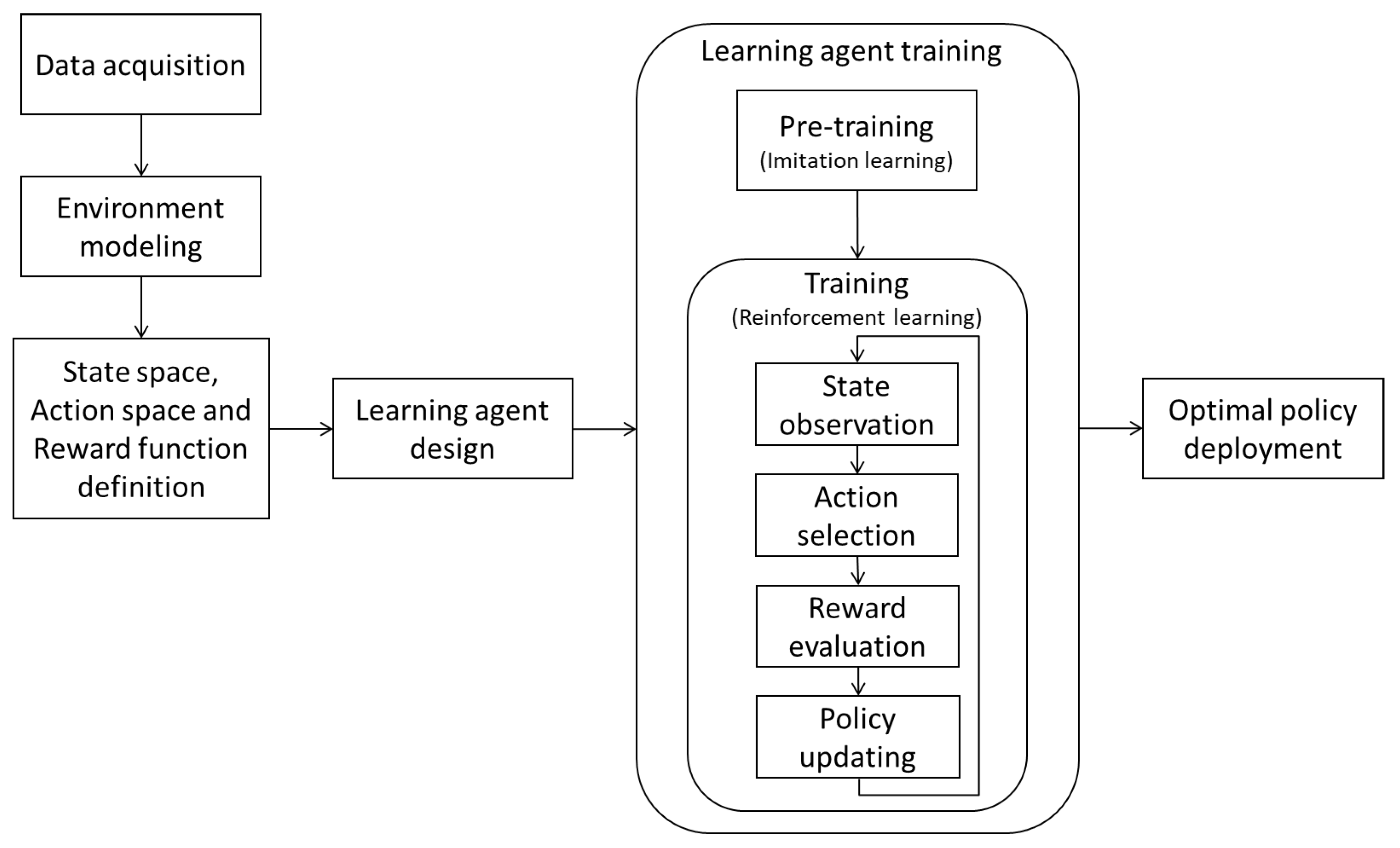
Figure 1 shows the schematic representation of the proposed approach for O&M optimization. First, the method requires the acquisition of the data needed to build a model of the environment. Then, the problem is formulated as a SDP and the state space, the action space and the reward function are defined. The next step is the development of, which requires the definition of the DANN architecture and its training by means of imitation learning and RL. After the optimal O&M policy has been discovered, it can be deployed to the real-world system.
3.1. Problem Formulation
Since the goodness of an O&M action does not depend exclusively on the state the environment enters as the result of the decision taken at the present decision instant, but rather on the whole sequence of states entered, performed actions and obtained rewards throughout the long-time horizon, the problem is here formulated as a SDP.
3.1.1. State Space
In SDP, the state space contains the information about the system and its environment which can influence the decision. In this work, we consider relevant for the optimization of the wind farm O&M: (a) the predicted RULs of the L wind WTs provided by the PHM systems, , (b) the prediction of the WTs power production for the current and J following days, ; notice that the use of the future power production values within the optimization allows predicting the loss of revenue in case of maintenance or failure, which is a key driver of the overall costs, (c) the time interval needed to complete the current maintenance action on each WT, , which are related to the time at which the maintenance crews will be available again and (d) the current time t. The system state at time t is, then, defined by the vector .
3.1.2. Action Space
The available O&M decisions are organized in the vector , where , indicates that the destination of the selected maintenance crew is component l, whereas the last action corresponds to the decision of sending the maintenance crew to the depot. At every time t, a decision is taken about the next destination of each maintenance crew. Namely, the learning agent returns as output a vector of C destinations, one per crew. If one of the L units is selected as destination, the maintenance intervention (preventive or corrective) starts as soon as the crew reaches the unit, whereas if the depot is selected, the crew will start waiting for a new assignment as soon as it arrives at destination. When a maintenance operation starts, the corresponding component is stopped and its power production becomes 0.
3.1.3. Reward Function
At every decision instant
t, the decision maker receives a reward
defined by:
where
is the maintenance costs at time
t, being
and
two boolean variables representing the type of maintenance action performed on the
l-th component at time
t and being
a boolean variable representing if one of the
C maintenance crews has been assigned to the maintenance of the
l-th component at time
t.
3.2. Reinforcement Learning
RL is a branch of machine learning in which a learning agent interacts with an environment to optimize a reward, i.e., a feedback that the environment gives to the agent. RL is based on the psychology principle known as “Law of Effect”, according to which actions that provide positive effects in a particular situation will more probably be performed again in that situation and actions that provide negative effects will less probably be performed again in that situation [
15]. The general algorithm of RL is shown in
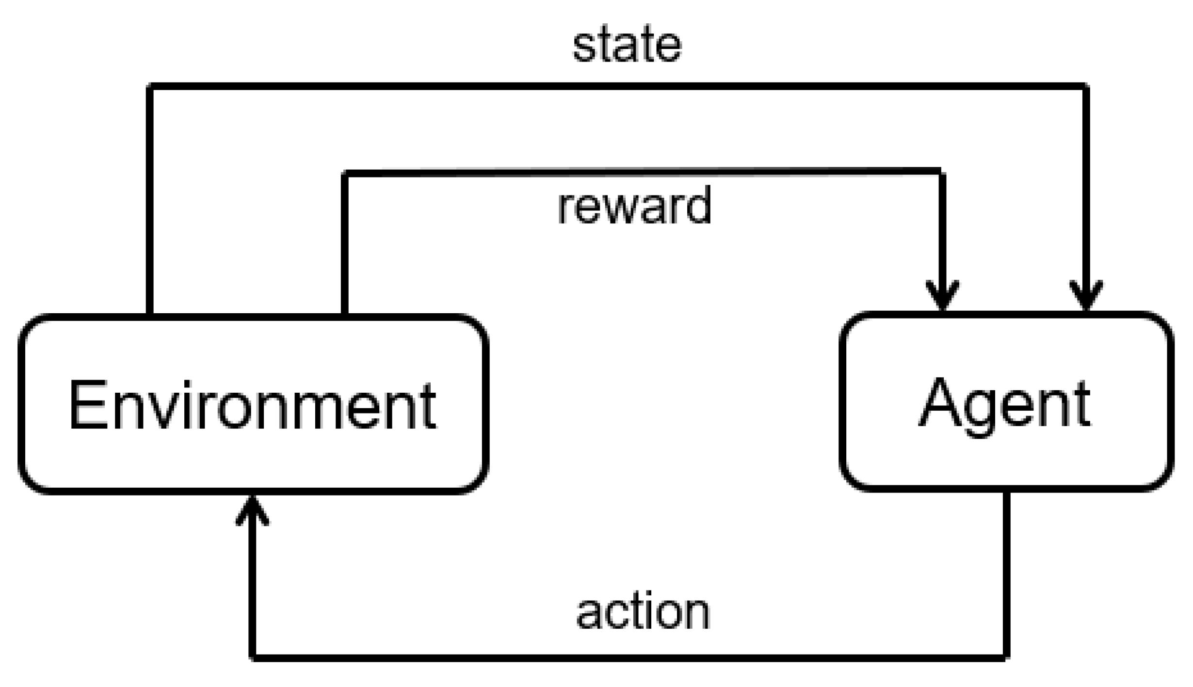
Figure 2. The agent is the decision maker and the environment is everything the agent can interact with. At every step, the agent observes the state of the environment and selects the action to be performed. Every action the agent takes causes the transition of the environment to a new state and the computation of a reward that is provided to the agent and can be used to update the policy, i.e., the function used to select the actions. The learning process is iterated to discover the policy which allows the maximization of the overall reward value [
15].
Several algorithmic implementation of RL have been proposed in literature. They can be divided into the three groups of
value function,
policy search and
Actor–Critic methods [
29]. Value function methods learn the value of being in a particular state and, then, select the optimal action according to estimated state values. They are usually characterized by slow convergence rate and fail on many simple problems [
26]. A well known example of a value function method is Deep Q-Networks (DQN) [
30], in which a deep neural network is used to approximate the value function.
Policy search methods directly look for the optimal policy by learning a parameterized policy through which optimal actions are selected. The update of the policy parameters can be performed by means of gradient-free methods, e.g., evolutionary algorithms, or gradient-based methods, e.g., REINFORCE algorithms [
31]. Even if these methods have been shown to be effective in high dimensional or continuous actions spaces, they typically suffer from large variance in the estimates of the gradient and tend to converge to local optima [
16].
Actor–Critic methods learn both the value function and the policy in an attempt of combining the strong points of value function and policy search methods [
29]. Actor–Critic methods consist of two models: the actor model carries out the task of learning the policy by selecting the action to be performed in every environment state, whereas the critic model learns to evaluate whether the action taken by the actor leads to a better or a worse state of the environment and gives its feedback to the actor, allowing updating the current policy and selecting improved actions.
In this work, we have employed proximal policy optimization (PPO) [
26], which is an Actor–Critic method. In PPO, an estimator of the gradient is computed by differentiating a surrogate objective defined as the minimum between an unclipped and a clipped version of a function of the reward [
26]. The minimum is used to define a lower, i.e., pessimistic, bound on the unclipped objective and the clipping is used to penalize too large policy update, avoiding second-order approximations of a constraint, as in Trust Region Policy Optimization (TRPO) [
32]. PPO has been chosen among the possible RL algorithms since, despite its relative simplicity of implementation, it has been shown to outperform many state-of-the-art approaches in several research fields such as computer science [
26], autonomous transportation [
33] and robotics [
34].
When the state space is very large, it can be hard for the agent to find the optimal action to be performed in every state, starting from a random initialization of the neural network weights. This problem can be tackled by exploiting domain knowledge to lead the learning process. One popular approach to do this is
reward shaping [
35], which consists in building an ad hoc reward function to provide frequent additional feedback on suitable actions, so that promising behaviors can be discovered in the early stages of the learning process. A drawback of reward shaping is that it requires the tuning of the reward function parameters, which, if not properly performed, can lead to unexpected outcomes. Another possible approach is
state-action similarity solutions [
36], which is inspired by constructivism and allows including the domain knowledge by engineering state-action similarity functions to cluster state-action pairs. In this work, we resort to
imitation learning [
37], which consists in providing the agent some demonstrations of a state-of-the-art policy and initially training the agent to reproduce it by means of supervised learning. We have selected imitation learning since it facilitates the problem of teaching complex tasks to a learning agent by reducing it to the one of providing demonstrations, without the need for explicitly designing reward functions [
37]. Then, RL is used to conclude the learning process, allowing the improvement and the fine-tuning of the learnt policy.
4. Case Study
We consider a wind farm composed of
identical WTs equipped with PHM capabilities and operating over a time horizon
days. The failure time,
T, of each WT is sampled from an exponential distribution with failure rate
days
−1, obtained by modeling the WT as a series equivalent of sub-systems, whose failure rates are set equal to the values reported in [
38]. The predicted RUL,
R, is estimated at each time according to Equation (
2), assuming
days.
Searching for the optimal O&M policy by performing real interactions of the learning agent directly with the wind farm is practically unfeasible for economic, safety and time issues [
15]. In fact, due to the trial-and-error nature of the learning process, the agent would need to perform several times the actions suggested by the algorithm in order to explore their outcomes, and this leading to economically inconvenient and unsafe system management in the early stages of the learning process, when they are still not optimal. For this reason, the learning agent is trained on simulated power production data, without (negatively) affecting the real production process during the optimality search. The main characteristics of the real power productions, i.e., the periodicity of the wind speed and its stochasticity, are represented by:
where
,
,
days and
identifies the clipping operation to values between 0 and 1. The
function allows representing the of the wind speed and the noise
its stochasticity, whereas the clipping operation has been introduced to keep the value in the range [0, 1]. Since the time step,
t, used in this work is 1 day, Equation (
6) describes the monthly periodicity of the wind speed, whereas it neglects the daily and yearly periodicity. This is justified by the fact that the daily and yearly periods are respectively too small and too big to influence the decisions which are taken each day. Also, although the time evolution of the wind speed is more complex than a sinusoidal function with an added Gaussian noise, the approximation taken allows showing the capability of the method to deal with variable environmental conditions. Notice that the same learning agent can be applied to more complex models of the wind speed or to real wind speed data of a specific existing plant. Since the learning agent does not receive in input information on the wind speed periodicity, but only the prediction of the power production obtained by applying Equation (
3), the overall performance of the method is not expected to be significantly affected by approximating the wind speed using Equation (
6). For this reason, future work will be developed to consider more advanced models of the power production, such as a Markovian model [
39] whose parameters can be identified using real production data. At every decision time
t, the value of the predicted power production for the present and next
j days, with
, is set according to Equation (
3), where
and
days.
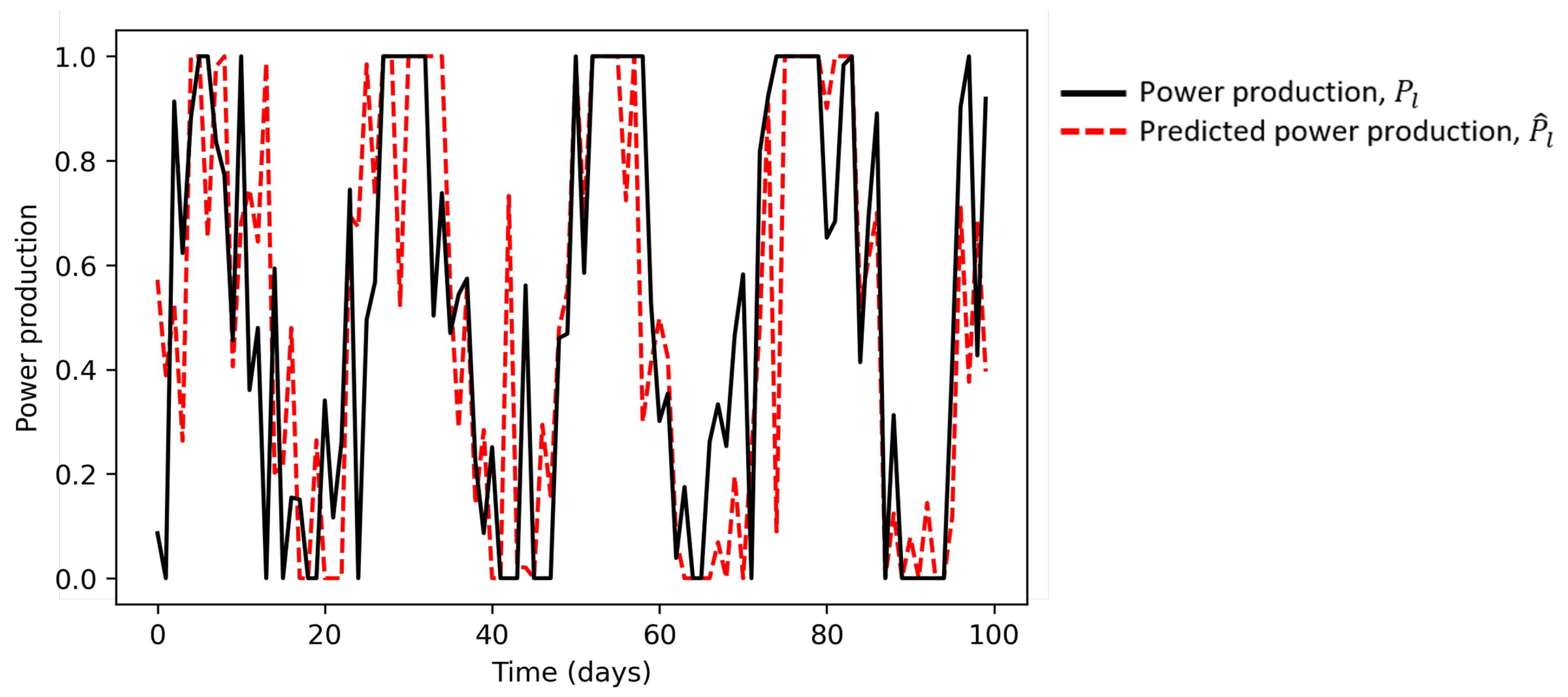
Figure 3 shows a simulated trajectory of the power production obtained using Equation (
6) and the corresponding values predicted one step ahead using Equation (
3). Considering the two trajectories at a generic time
, the former represents the ground-truth production at time
, which is unknown at the present time
, whereas the latter represents the prediction of the production at time
, which is the only information that can be used by the learning agent for the decision of the action to be performed. Notice that the mismatch between the two curves is due to the predicting error, which, in this work, has been modeled with a Gaussian noise. A limitation of this modeling choice is that the prediction error is not expected to be time-independent, since the model prediction error has been shown to vary substantially with different environmental conditions, e.g., between winter and summer [
40,
41].
In this work, we perform three experiments changing the number of available maintenance crews .
The maintenance times are sampled from exponential distributions with repair rate days−1 and days−1, for preventive and corrective maintenance, respectively.
Finally, the income
K is set equal to 96, whereas the cost of PM and CM actions are
and
[
42], all in arbitrary units.
We resort to a feedforward neural network characterized by 2 hidden layers of 64 neurons each, as learning agent. The imitation learning step is performed by simulating 500 predictive maintenance trajectories and training the learning agent for 40 epochs. The PPO clipping hyperparameters is set equal to 0.2 and training lasts for a total of time steps using 8 actors in parallel. The computations have been performed on two Intel® Xeon® CPUs at 2.30 GHz with 13 GB of RAM using Python.
5. Results
The proposed RL-based policy is validated by means of the comparison with the following three state-of-the-art maintenance strategies:
corrective—maintenance interventions are performed exclusively after a turbine failure;
scheduled—maintenance interventions are scheduled at regular intervals;
predictive—maintenance interventions are performed when the turbine RUL prediction is smaller than a user-defined threshold.
The scheduled and predictive maintenance strategies require the setting of the time interval between two consecutive maintenance interventions and the RUL threshold, respectively, This is done by optimizing the wind farm profit over 250 episodes using the Tree-structured Parzen Estimator (TPE) algorithm [
43].
The performance of the considered strategies are evaluated by performing 100 test episodes characterized by different random initializations of the WT health states. The average value and standard deviation of the profit over 100 episodes are reported in
Table 1, in arbitrary units. First of all, notice that the predictive and RL policies provide better performances than the corrective and scheduled maintenance policies, which are the maintenance strategies most commonly applied to wind farms [
44,
45,
46,
47,
48], with a 40% increment of the profit when the RUL predictions provided by the PHM systems are used. The scheduled maintenance is characterized by performance similar to corrective maintenance, due to the exponential behavior of the WTs failure times. The proposed RL policy outperforms the predictive maintenance strategy of about 3% when a single maintenance crew is available, whereas the gain becomes lower when the number of available maintenance crews increases. This result confirms that the proposed method is able to optimize the O&M policy in the most challenging situation of limited crew-availability. Also, the proposed method allows obtaining with one crew the same profit obtained by the predictive maintenance strategy with three crews, which indicates that the RL policy allows a more effective management of the single maintenance crew than the other maintenance strategies. Also, since in this work the costs related to the crews employment and management have been neglected, the reduction of the maintenance crews allows remarkably reducing the overall costs.
The last column of
Table 1 reports the computation times needed for the optimization of the selected maintenance strategies. The computation time of the proposed method, which requires the training of a deep neural network, is an order of magnitude larger than the time needed for the optimization of the other policies, which only require the execution of the TPE algorithm. Notice, however, that, once the PPO has identified the optimal policy, i.e., the learning agent has been trained, the proposed method can be applied in almost real time to obtain the action to be performed given the environment data.
Notice that the proposed approach can be used to estimate the optimal number of maintenance crews, , to be employed by a wind farm. This requires to:
Repeat the training and test of the learning agent with different number of maintenance crews, C, and estimate the corresponding ;
Find the optimal number of maintenance crews, , as:
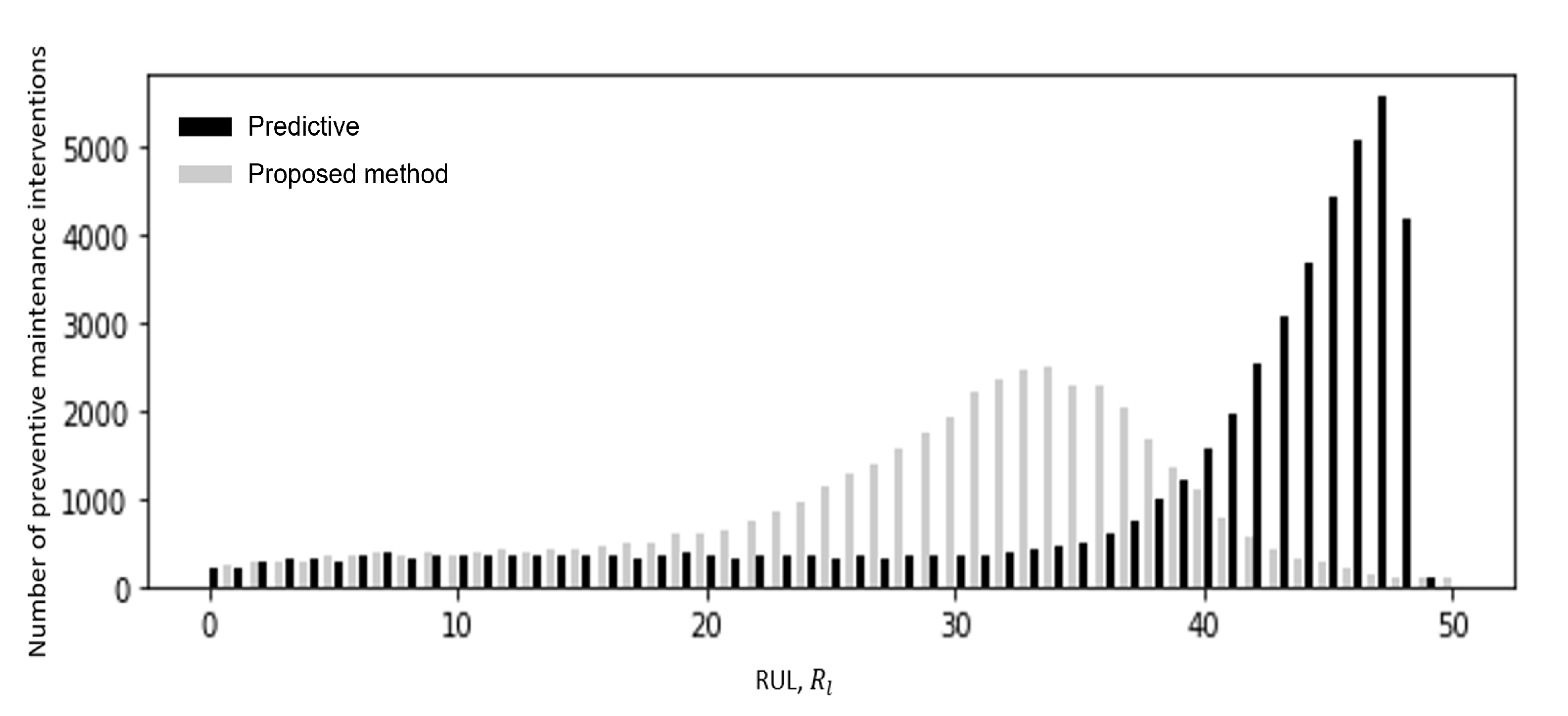
Figure 4 shows the number of maintenance interventions performed by predictive and RL-based maintenance policies as a function of the RUL. Even if the RL agent has been pre-trained in the imitation learning phase using the predictive policy, the RL agent tends to postpone preventive maintenance interventions with respect to predictive maintenance, which has to anticipate the maintenance interventions to avoid failures caused by the unavailability of the maintenance crews (
Figure 4). Notice the truncated distribution of the intervention times of the predictive maintenance strategy, which is due to the fact that the method optimizes the threshold on the RUL prediction, i.e., the time at which the intervention is required. The distribution shows that in many cases the maintenance interventions are postponed due to the unavailability of maintenance crews and, therefore, performed when the RUL is smaller than the threshold. The distribution is also influenced by the RUL prediction error, which causes a small mismatch between the real RUL and the predicted one. The distribution of the intervention times of the proposed method is instead more symmetric due to the fact that the RL policy is not based on the definition of a threshold on the RUL but on a combination of different factors. In particular, the right-hand tail is caused by maintenance opportunities generated by the prediction of low power production for the next days, which can be exploited by anticipating maintenance, whereas the left-hand tail is caused by the maintenance crew unavailability, as for the predictive maintenance.
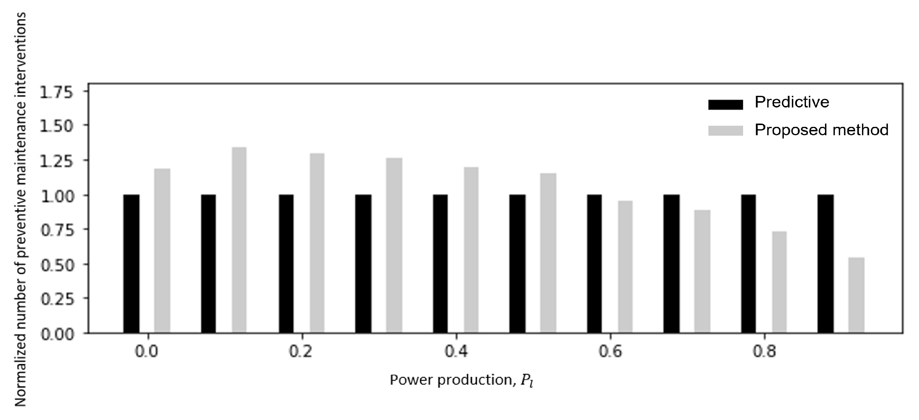
Figure 5 shows the number of maintenance interventions performed as a function of the current power production, normalized by the number of times each power production value is verified, in the case of
C = 1 maintenance crew. Differently from the predictive policy, the RL-based policy shows a dependence between the number of interventions and the power production (
Figure 5). As expected, the largest number of interventions is performed when the power production will be low.
Figure 6 and
Figure 7 show the number of maintenance interventions as a function of RUL and power production, considering the availability of
C = 3 maintenance crews. In this case, the two policies are very similar with respect to the dependence on the RUL.
Finally, we propose a comparison with the ideal, non-realistic, case in which the PHM system predicts the exact RUL, without any error, i.e., days. Independently from the number of available maintenance crews, the achieved profit is around , which is just 2% higher than the one achieved by RL in presence of error in the RUL prediction. This shows the capability of O&M policy of managing the prediction errors of the PHM systems.
5.1. Analysis of the Robustness of the O&M Policy with Respect to Variation of the WTs Failure Rate and Maintenance Costs
We investigate the effect of modifications of the WTs failure rate (
Section 5.1.1) and of the preventive maintenance cost (
Section 5.1.2) on the selection of the optimal O&M policy. In both cases, two different studies are performed, as follows:
the first study is performed without re-training the learning agent, so as to assess the robustness of the O&M policy with respect to the unavoidable mismatch between the estimation of the environment characteristics, which are used for the policy definition, and the real environment to which the policy is applied;
the second study is performed with re-training of the learning agent, so as to assess the capability of the proposed method of identifying the optimal O&M policy in different environments.
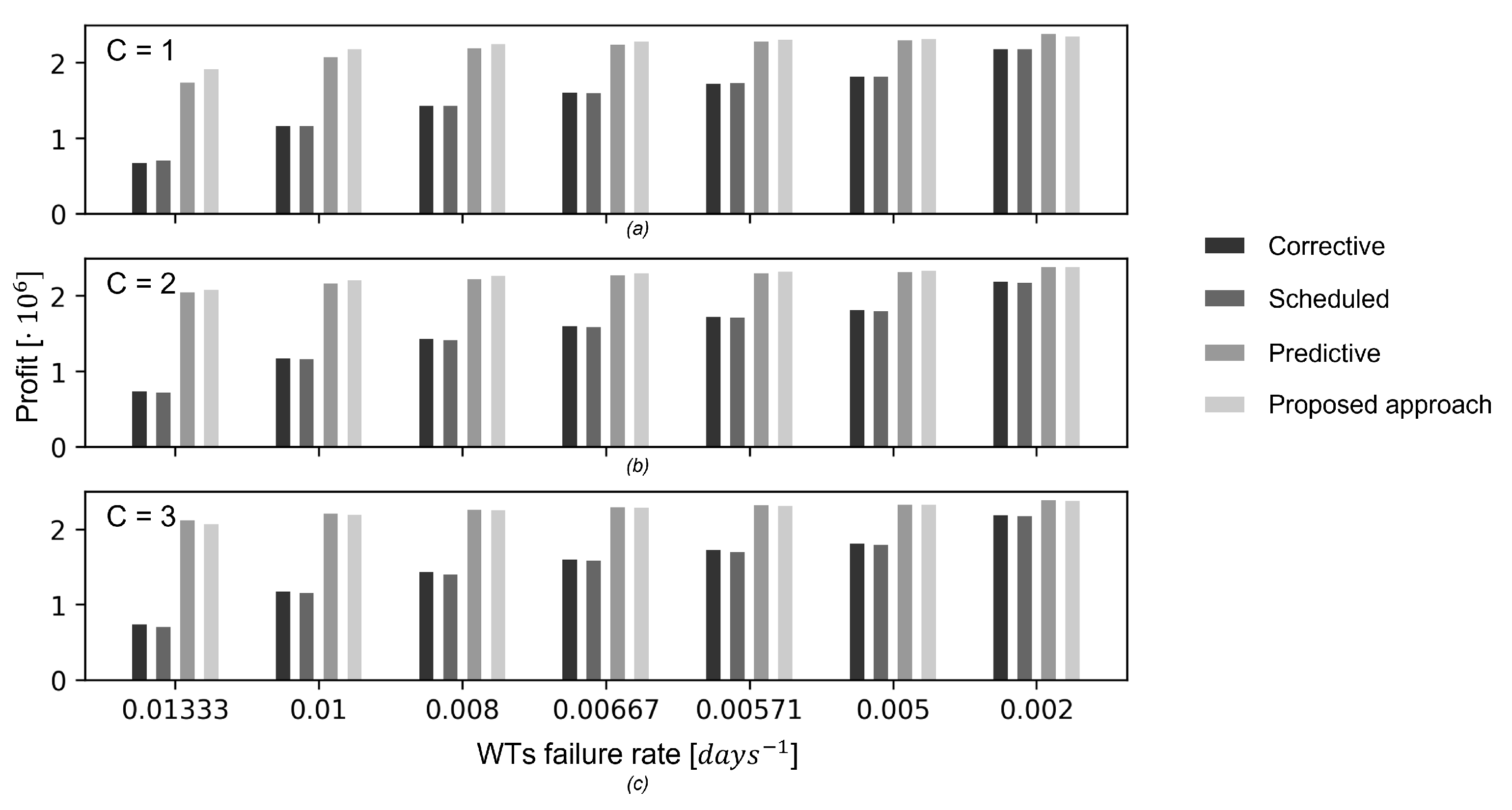
5.1.1. Dependence on WTs Failure Rate
Figure 8 shows the average profit obtained in the study (1) by the considered policies as function of the WTs failure rate over the test episodes. Similarly to what has been done for the proposed method, also the threshold of the predictive maintenance policy has not been re-optimized. As expected, the larger the WTs failure rate, the smaller is the profit for all the maintenance policies. Most importantly, the performance of the proposed method remains the most satisfactory and more robust with respect to variations of the WTs failure rate. This is due to the fact that the system state vector, which contains the WTs RULs, implicitly informs the learning agent about the true WTs failure rates. Furthermore, as shown in the previous Section, the policy discovered by the proposed method does not exclusively rely on the WTs RULs, but rather on the combinations of different aspects, such as the exploitation of opportunities of low power production, that make the policy more robust to variations of the real WTs failure rate.
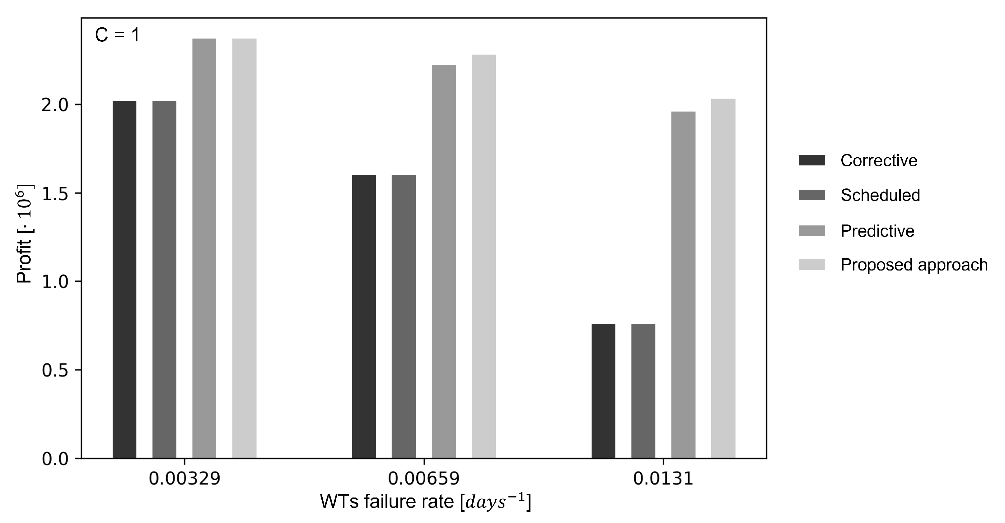
With respect to the study (2), the cases in which the failure rate is half and double of the value considered in
Section 4 (
days
−1 and
days
−1, respectively) have been considered. Since the results of
Section 5 have highlighted that the most interesting case is the one characterized by limited maintenance crew availability, we limit the analysis to the case with one maintenance crew available (
C = 1). Similarly to what has been done in this case for the proposed method, the threshold of the predictive maintenance policy has been re-optimized. The obtained performances are shown in
Figure 9. It can be noticed that the proposed method outperforms the predictive maintenance policy when the failure rate is doubled, whereas it obtains a performance very similar to the predictive maintenance policy when the failure rate is halved. This is due to the fact that when the failure rate is small, the maintenance costs are remarkably reduced, and, therefore, the profit is less influenced by the maintenance cost.
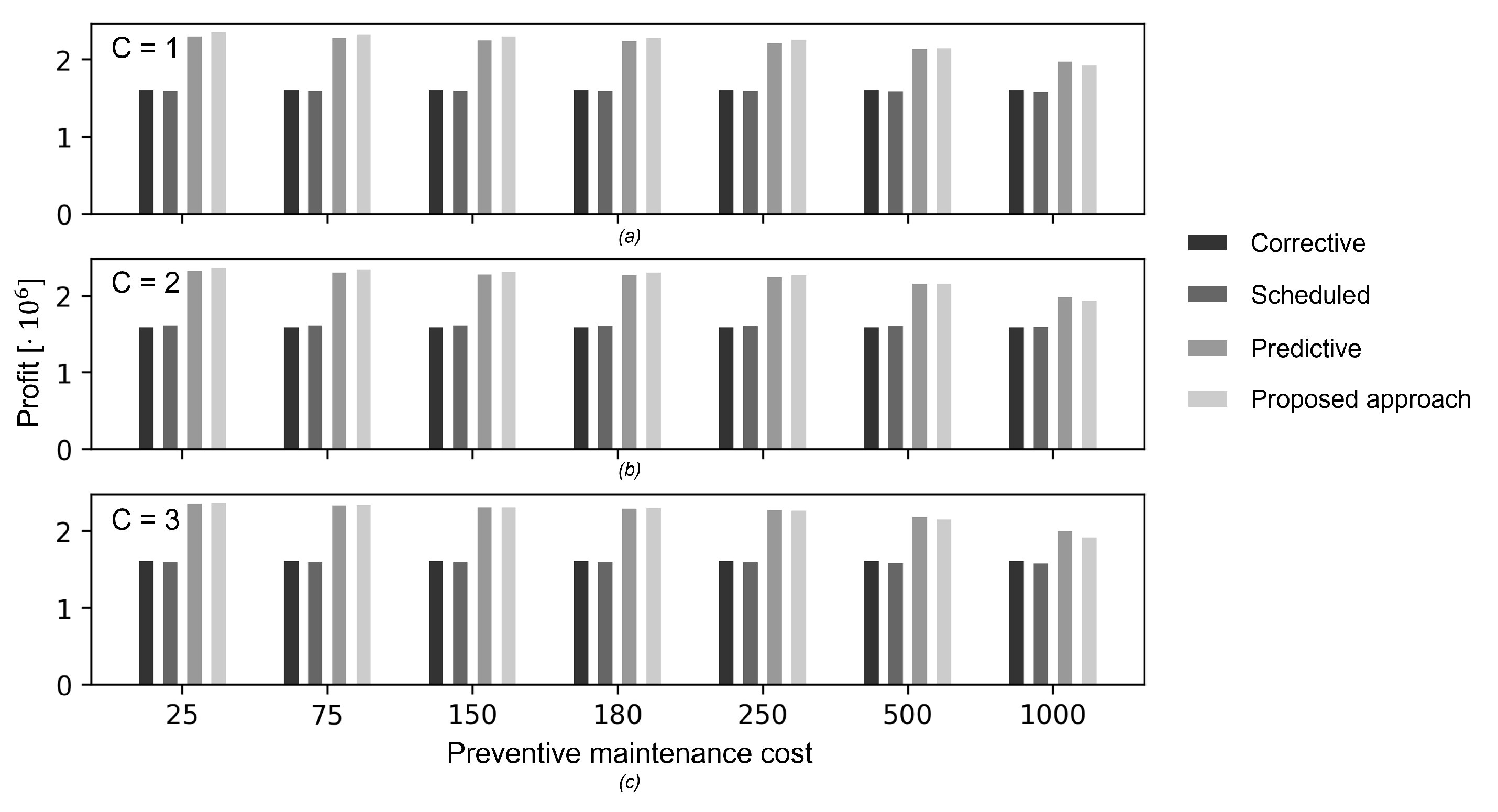
5.1.2. Dependence on Preventive Maintenance Cost
We repeat the analysis of
Section 5.1.1 considering the preventive maintenance cost parameter.
Figure 10 shows the average profit obtained in the study (1) as function of the preventive maintenance cost. As expected, the larger is the cost, the smaller is the profit for all the maintenance policies. Most importantly, the performance of the proposed method remains the most satisfactory and more robust with respect to reductions of the preventive maintenance cost, whereas the profit rapidly decreases as the cost increases, independently of the number of maintenance crews available. This is because the preventive maintenance cost is only contained in the reward function (Equation (
5)) and, therefore, the learning agent is unaware of its variation during the test episodes. Then, the outcome of this study highlights the importance of correctly estimating the cost of the maintenance interventions before training the learning agent, since incorrect values can lead to sub-optimal O&M policies. In the study (2), we consider the cases in which the preventive maintenance cost is one tenth and ten times the value considered in
Section 4 (
and
, respectively). The obtained performances are shown in
Figure 11. Since the learning agent is now aware of the correct value of the preventive maintenance cost, the proposed approach slightly outperforms the predictive maintenance policy for all the considered cost values. These results show the capability of the proposed approach to converge to an optimal policy, particularly if the correct value of preventive maintenance cost is provided during training.
6. Conclusions
In this paper we have developed a PPO-based approach for the optimization of the O&M policy of WTs equipped with PHM capabilities, in wind farms with multiple maintenance crews available. A deep neural network is trained to learn the best action to be performed at each decision instance, considering all the available information about the system and its environment.
The proposed approach has been tested on a wind farm and has been shown to provide an O&M policy which outperforms state-of-the-art policies. The effectiveness of the identified policy is confirmed by the fact that in case of a limited number of available maintenance crews it provides similar total plant power production of scheduled and predictive maintenance strategies relying on more maintenance crews. Then, the application of the proposed approach to wind farms is expected to allow improving the total profit over the plants lifetime, reducing the use of resources needed for maintenance.
The effect of the variations of two critical parameters for the definition of the maintenance policy, i.e., the WTs failure rate and the preventive maintenance cost, has been investigated. The obtained results have shown that the proposed approach is robust with respect to variations of WTs failure rate and it less affected then other maintenance methods by error in the WTs failure rate estimations, especially when few maintenance crews are available. On the other side, a correct estimation of preventive maintenance cost is needed to properly set the O&M policy since small variations of the preventive maintenance cost have been shown to induce a remarkable decrease of the performance. Also, the applicability of the proposed method to a large set of possible environments has been confirmed.
Future work will consider the application of the proposed approach to systems characterized by more complex environments. In particular, the WTs will be modeled as complex engineering systems composed of several interacting components, each one characterized by different degradation behaviour, failure severity and impact on the power production. Also, real wind speed data will be used to estimate the power produced by the wind farm and new environment parameters, such as the power demand, will be added to the state space. Finally, a study to identify the optimal number of maintenance crews for the wind farm O&M management will be conducted.
On the other hand, logistics decisions need to be intertwined with Operation and Maintenance (O&M) decisions.
Intuitively, the PHM estimations can be used to optimize the decisions on the unit Operation and Maintenance (O&M), which, in turn, influence the equipment degradation evolution itself [
13]. This brings big opportunities, because the optimization of the O&M strategy allows optimizing the of the system. Improvement of logistics is among the main expected benefit from prognostics and health management (PHM): the knowledge of the remaining useful life (RUL) allows organizing logistics for providing the right part to the right place at the right time. This is fundamental for setting efficient, just-in-time and just-right maintenance strategies, with consequent reduction of system downtimes. The logistic issue is emphasized in case of facilities spread across large areas, with whether conditions constraining the maintenance items reachability, such as off-shore Wind turbine plants (OSWTP). Although the benefit of PHM to reduce logistics-related downtime is intuitive,
An O&M strategy is optimal only if it yields the largest benefit in terms of safety and economics. Since the decision taken at the present time will influence the system state at the next time, RL considers the O&M decision taken at the present time to be optimal only if an optimal decision will be taken also at the next decision time. By iteratively applying this reasoning, the sequence of decisions generating the expected maximum profit can be defined.


